Abstract
The Lax pairs of the higher-order Gerdjikov–Ivanov (HOGI) equation are extended to the multi-component formula. Then, we first derive four different types of nonlocal group reductions to this new system. To construct the solution of these four nonlocal equations, we utilize the Riemann–Hilbert method. Compared to the local HOGI equation, the solutions of nonlocal equations not only depend on the local spatial and time variables, but also the nonlocal variables. To exhibit the dynamic behavior, we consider the reverse-spacetime multi-component HOGI equation and its Riemann–Hilbert problem. When the Riemann–Hilbert problem is regular, the integral form solution can be given. Conversely, the exact solutions can be obtained explicitly. Finally, as concrete examples, the periodic solutions of the two-component nonlocal HOGI equation are given, which is different from the local equation.
1. Introduction
In natural science and engineering technology, it is widely acknowledged that numerous phenomena are nonlinear and cannot be explained only by simple linear systems. Nonlinear systems, characterized by their nonlinear terms, provide a more precise depiction of these intricate phenomena compared to linear systems, and thus more accurately reflect the nature of these phenomena. Integrable systems include a special class of nonlinear partial differential equations (nPDEs), which have been widely considered because of their many good properties and algebraic structures [1,2,3]. Among many integrable systems, there are two most important equations, namely the nonlinear Schrödinger (NLS) equation and derivative NLS equation, which can be derived from the AKNS hierarchy and KN hierarchy, respectively. The NLS equation plays an important role in many fields such as water waves, nonlinear optics, and so on [4,5,6]. When the higher-order nonlinear effects are considered, the derivative NLS equations are seen as long-wave, small-amplitude models in a wide range of fields, including quantum field theory and short light pulse [7,8,9]. The derivative NLS equation can be generally represented as
where denotes the complex conjugation of u [10]. When and , Equation (1) can be reduced to the Kaup–Newell (KN) equation, also known as DNLS I, which is derived from the magneto-hydrodynamic equations with the Hall effect [11]. When , Equation (1) transforms to the Chen–Lee–Liu (CLL) equation, also called DNLS II, which is an optical model of ultrashort pulses [12]. When , Equation (1) changes into the Gerdjikov–Ivanov (GI) equation, also called DNLS III, which is applied to model Alfvén waves propagating parallel to the ambient magnetic field [13]. Three types of the derivative NLS equation can be transformed through Gauge transformations, CLLKNGI. The CLL equation transforms into the KN equation through the Gauge transformation (a) [14], and making another Gauge transformation (b) [15], the KN equation yields the GI equation. Due to the complexity of the integral terms involved in Gauge transformations and the alteration of Lax pairs after applying Gauge changes, each of them deserves separate investigation. Therefore, it is simpler and more convenient to deal with them separately. For example, there are several individual studies on KN, CLL, and GI equations [16,17,18]. For the CLL equation, Zhang et al., gave the n-fold Darboux transformations in the determinant form and successfully obtained the rogue wave and multi-rogue wave solutions through these transformations [17]. For the GI equation, Fan gave the soliton-like solutions by the n-fold Darboux transformation [16], and He et al., obtained the rogue wave solutions from a periodic "seed" by the two-fold Darboux transformation [18]. So far, there are some studies on these three equations, but most are local cases.
In recent years, nonlocal integrable systems, largely viewed as variants of classical local integrable systems, have developed into one of the new hot topics in soliton theory. More importantly, the discovery of nonlocal integrable systems stems from a hot research area in modern physics: parity-time () symmetry. In 1998, Bender et al., discovered an important relationship between the existence of all real eigenvalues for a non-Hermitian system and -symmetry, which has nonlocal features involved simultaneously at two mirror symmetry points and [19]. Ablowitz et al., proposed the concept of nonlocal integrable systems [20]. Then, Yan studied the -symmetry nonlocal and local integrable vector nonlinear Schrödinger (NLS) equations under different reduction conditions [21]. Musslimani et al., proposed the Cauchy problem and the theory of inverse scattering transforms for nonlocal NLS equations [22]. Lou et al., proposed the Alice–Bob system based on the -symmetry theory and discovered its multi-soliton solution [23]. Chow et al., discussed breather and rogue wave solutions for third-order nonlocal partial differential equations [24]. Gerdjikov et al., discussed the integrable properties of nonlocal NLS equations [25]. Rao et al., applied the KP hierarchy reduction method to study the nonlocal Davey–Stewartson I equation with nonzero background [26]. Recently, Ma et al., introduced -symmetry into the multi-component integrable systems and studied the Riemann–Hilbert problem of these integrable systems [27,28].
In this paper, we mainly study a reverse-spacetime multi-component higher-order Gerdjikov–Ivanov (mHOGI) equation
where , is an invertible matrix, and T represents matrix transposition. The local GI equations have been extensively studied, such as the decomposition of GI equation [29], Wronskian solution [30], hierarchy structure [31], Darboux transformation [16], and Gauge transformation [32]. Compared to local GI equations, nonlocal higher-order GI equations have different dynamical behavior due to nonlocal terms and higher-order dispersion. More importantly, nonlocal multi-component GI equations result in richer features across different components. Therefore, we intend to study the nonlocal multi-component GI equation and obtain the exact solutions by the Riemann–Hilbert (RH) method.
This paper starts with the following structure. Section 2 gives four different types of nonlocal group reductions of the mHOGI equation and then derives the reverse-spacetime mHOGI equation through the Lax pairs, compatibility condition, and nonlocal group reduction. Section 3 analyzes the analyticity of Jost’s solution to the reverse-spacetime mHOGI equation, establishes its RH problem, and gives the symmetries of the eigenfunction matrix and the scattering data. In Section 4, when the determinant of the eigenfunction matrix is not zero, the integral form solution is given by the Sokhotski–Plemelj formula. Conversely, exact solutions are obtained, and the first three exact solutions of the nonlocal 2-component GI equation are given.
2. Nonlocal Multi-Component Higher-Order Gerdjikov–Ivanov Equation
The Lax pairs of scalar GI equations have been well known and studied, but the reverse-spacetime mHOGI equation has not been studied. Therefore, we will build a reverse-spacetime mHOGI equation by nonlocal group reduction in this section.
Firstly, we introduce the Lax pairs of mHOGI equation
with
where
Here, stands for spectral parameter, is defined in Equation (2). This Lax pair can obtain the mHOGI equation
by zero curvature equation
Then, we list four different types of nonlocal group reductions.
Case 1: The nonlocal group reduction is
and the corresponding potential reduction is
where and .
Case 2: The nonlocal group reduction is
and the corresponding potential reduction is
where
Case 3: The nonlocal group reduction is
and the corresponding potential reduction is
where .
Case 4: The nonlocal group reduction is
and the corresponding potential reduction is
where .
In this paper, we mainly discuss a nonlocal group reduction about reverse-spacetime
as a concrete example to demonstrate the study of the Riemann–Hilbert problem to nonlocal mHOGI equation. This nonlocal group reduction is derived from case 2 when . According to Equation (4), it is easy to obtain
which equivalently leads to
Similarly, we can gain the reverse-spacetime group reduction of the time part
It is easy to know the nonlocal group reductions Equations (16) and (19) also satisfy the compatibility condition (7). Therefore, according to the Lax pairs, compatibility condition and nonlocal reduction, the reverse-spacetime mHOGI equation can be gained,
When , the reverse-spacetime two-component GI equation can be obtained,
3. Riemann–Hilbert Problem of the Reverse-Spacetime mHOGI Equation
In this section, we will analyze the analytical properties of the eigenfunction matrix to construct the RH problem of the reverse-spacetime mHOGI equation, discuss the symmetric properties of the scattering data, and present its time evolution.
Firstly, assuming that all the potentials rapidly vanish as , we can gain the reverse-spacetime mHOGI equation’s asymptotic behavior: . Then, we introduce a new function
It is straightforward to know that when , . Substituting this new function into Equation (3), we determine
According to the Liouville’s formula [33], we can gain
Then, we introduce two matrix Jost solutions of Equation (23) that satisfy
when , respectively. According to Equation (25), it is easy to gain that det for all x.
Combined with boundary conditions (26) and the parameter variation method, Equation (23) can be converted into the Volterra integral equation below [34]:
When we consider the analyticity of , it is easy to find from Equation (27) that the exponential factor is present in the first column of and the last n columns of involves only the exponential factor . Because and the exponential factor decays when , the first column of are analytic in . Because and the exponential factor decays when , the last n columns of is analytic in , and both allow analytical continuations to . Similarly, it is obvious that the first column of and the last n columns of are analytical in and , respectively (See Figure 1).
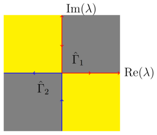
Figure 1.
The jump contour in the complex, where the red line denotes , the blue line denotes , the gray area represents , and the yellow area represents .
Since
are both solutions of Equation (3), there is a linear relationship between them
where is called the scattering matrix. The scattering matrix S satisfies
and det . Obviously, is analytically extended to , the rest of allow analytic extension to .
According to the analyticity of the Jost solution, we construct two matrix eigenfunctions , analytically continued to and , respectively. Let
we can make
where and are defined by
According to the analyticity of , is analytic in and continuous to . By inserting into Equation (29), the equation can be derived,
Then,
Similarly, we can use the adjoint spectral problems to construct the matrix eigenfunction , which is analytic in . Since det , is identified as the adjoint matrix. Therefore, we can obtain
Let
we can make
Similarly, it is clear that
where . It can be seen from the above formula that det.
Secondly, we examine the symmetries of some matrices. If is the matrix eigenfunction of the spatial spectrum problem Equation (23), then is its matrix adjoint eigenfunction, and they have the same eigenvalue . Therefore, based on nonlocal group reductions (17), it is easy to know that
presents another matrix adjoint eigenfunction associated with the same original eigenvalue , i.e., solves the adjoint spectral problem (33). Therefore, upon observing the asymptotic properties for at infinity for , the uniqueness of solutions tells us that
The jump matrix J carries basic scattering data from the scattering matrix and has the property .
The Jost solution satisfies another symmetry relation
namely,
It is visible that if is the zero of , then combined with the above m it can be shown that is another zero of . According to nonlocal group reductions, it can be shown that has two zeros, namely .
The time evolution of the time-dependent scattering coefficients is given by
and the rest of the scattering coefficients are all time-independent.
4. Solutions by the Riemann–Hilbert Method
In this section, the solutions of the reverse-spacetime mHOGI equation are gained by the RH method. When using the RH method to solve the equation, for the RH problem, there are two situations, one of which is the regular RH problem, namely and . In this case, for the general local initial conditions, the solutions of the reverse-spacetime mHOGI equation cannot be expressed explicitly, but the formal solution can be obtained by the Sokhotski–Plemelj formula. For this type, we can determine
Their boundary condition is that when ,
By the Plemelj formula, it is easy to obtain
where and is defined in Figure 1.
Theorem 1.
[Uniqueness Theorem of Solutions] If and are both solutions of Equation (44), .
Proof.
Now, we will prove the uniqueness of the solution. Assume that and are two different solutions of Equation (44); then, according to Equation (44), we know that , namely
If and are analytic in and , respectively, a matrix function in the entire plane is established by analytical continuation. Using Equation (45), it is evident that this analytic function converges to the identity matrix at . Liouville’s theorem is one of the fundamental theorems in complex functions, and its content can be simply described as “a bounded analytic integral function must be a constant function”. Therefore, combining Liouville’s theorem and the above description, we know that
namely , implying the uniqueness of the solution. □
Considering the symmetry and involution properties of and , we suppose that has zeros and has zeros . Here, we focus on the case of a single zero, that is, all zeros are simple. According to matrix theory, we can take
From Refs. [35,36,37], if the RH problems have canonical normalization conditions and zero structures (48), the problems can be solved. If , there is no reflection in the scattering data, namely . Hence, we can take the solutions as
where and
Since the space and time of solutions are independent of each other, using Equations (23) and (48), we have
Looking at Equation (48), we know that the vectors and are linearly related, namely
where is a constant. Similarly, we can determine
where is a constant. Without loss of generality, we take , then
where is independent of x and t.
Then, the large- expansions of are derived,
Then, we can obtain via Equation (49)
Combining Equations (58) and (59), the exact solutions of the reverse-spacetime mHOGI equation is obtained,
where the matrix is defined by Equation (50), and and , respectively.
Finally, as a concrete example, we give the three different solutions of the two-component nonlocal reverse-spacetime HOGI equation.
When , we take
where , and are arbitrary, and are arbitrary but nonzero.
When , we can derive the solution in Equation (60)
From the mathematical structure of the solution, it can be seen that solutions are singular outside of , and the solution can decay to a constant on .
When , the solution is rewritten as
where
Similarly, we find that the solutions are singular outside of , but in this case, the solutions degenerate into periodic wave solutions on .
When , the solution is rewritten as
where
with .
In the same way, we obtain the same conclusion as the case . Without loss of generality, choosing some specific values of or , we can give figures of periodic wave solutions with and (see Figure 2).
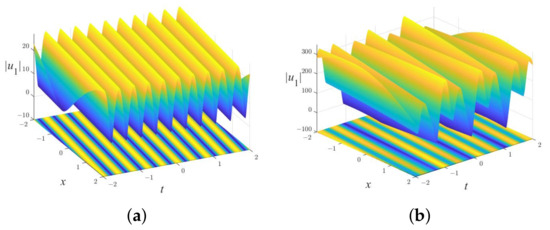
Figure 2.
Periodic wave solutions to the reverse-spacetime mHOGI equation: (a) ; (b) .
5. Discussion
In this paper, we list four different types of nonlocal group reductions of the multi-component higher-order Gerdjikov–Ivanov equation. Then, a class of nonlocal reverse-spacetime mHOGI equation and its Riemann–Hilbert problem are obtained under the parity-time transformation (). The main analysis is based on Riemann–Hilbert problems associated with a kind of arbitrary-order matrix spectral problems with matrix potentials under zero background. Upon obtaining the exact solution to this equation, we explore two types of the Riemann–Hilbert problem. One is the regular Riemann–Hilbert problem. At the same time, the other one is the non-regular Riemann–Hilbert problem with a reflectionless scattering problem. Whenever the transition matrix J equates to an identity matrix, exact solutions of the nonlocal reverse-spacetime mHOGI equation are presented the explicit formulas. Finally, as specific examples, the first three solutions to the two-component nonlocal reverse-spacetime HOGI equation are shown. We find that under this parity-time transformation, there are periodic wave solutions only on , and in other regions, the solutions are singular.
In this paper, we mainly focused on the nonlocal multi-component HOGI equation with the zero boundary condition. In future, we will consider the nonlocal multi-component HOGI equation with the non-zero boundary condition. Compared with the zero boundary condition, the Riemann–Hilbert problem with non-zero boundary becomes more complex, especially for multi-component systems. The main reason is that the spectral distribution becomes more complex under the non-zero boundary condition, and the forms of solutions corresponding to spectral points become more diversified. The periodic wave solutions are constructed when the Riemann–Hilbert problem is non-regular. Conversely, when the Riemann–Hilbert problem is regular, we can analyze the asymptotics of the solutions. In Refs. [38,39], the authors studied the long-time asymptotics for the nonlocal mKdV equation. And in Ref. [40], the authors analyzed the long-time asymptotics for the integrable nonlocal Lakshmanan–Porsezian–Daniel equation. Following this idea, the long-time aymptotics of the nonlocal multi-component HOGI equation will be studied in future work.
Author Contributions
Conceptualization, H.D.; methodology, Y.F.; software, Y.Z.; validation, Y.Z., H.D. and J.L.; formal analysis, H.D.; resources, Y.F.; writing—original draft preparation, H.D. and J.L.; writing—review and editing, Y.Z.; visualization, Y.Z. All authors have read and agreed to the published version of the manuscript.
Funding
This research was funded by the National Natural Science Foundation of China grant number 12305003, 12101246.
Data Availability Statement
No new data were created or analyzed in this study. Data sharing is not applicable to this article.
Acknowledgments
The authors would like to express their gratitude to the editors and reviewers for their valuable contributions to enhancing the quality of this paper.
Conflicts of Interest
The authors have no conflicts of interest to declare.
References
- Gardner, C.S.; Greene, M.; Kruskal, M.D.; Miura, R.M. Method for solving the Korteweg-de Vries equation. Phys. Rev. Lett. 1967, 19, 1095–1149. [Google Scholar] [CrossRef]
- Zakharov, V.E.; Shabat, A.B. Exact theory of two-dimensional self-focusing and one-dimensional self-modulation of waves in nonlinear media. Sov. Phys. JETP 1972, 34, 62–69. [Google Scholar]
- Date, E.; Jimbo, M.; Kashiwara, M.; Miwa, T. KP hierarchies of orthogonal and symplectic typetransformation groups for soliton equations VI. J. Phys. Soc. Jpn. 1981, 50, 3813–3818. [Google Scholar] [CrossRef]
- Thomas, R.; Kharif, C.; Manna, M. A nonlinear Schrödinger equation for water waves on finite depth with constant vorticity. Phys. Fluids 2012, 24, 66–84. [Google Scholar] [CrossRef]
- Chabchoub, A.; Kibler, B.; Finot, C.; Millot, G.; Onorato, M.; Dudley, J.M.; Babanin, A.V. The nonlinear Schrödinger equation and the propagation of weakly nonlinear waves in optical fibers and on the water surface. Ann. Phys. 2015, 361, 490–500. [Google Scholar] [CrossRef]
- Wang, M.M.; Chen, Y. Dynamic behaviors of general n-solitons for the nonlocal generalized nonlinear Schrödinger equation. Nonlinear Dyn. 2021, 104, 2621–2638. [Google Scholar] [CrossRef]
- Clarkson, P.A.; Tuszynski, J.A. Exact solutions of the multidimensional derivative nonlinear Schrödinger equation for many-body systems of criticality. J. Phys. A 1990, 23, 1171–1196. [Google Scholar] [CrossRef]
- Mio, K.; Ogino, T.; Minami, K.; Takeda, S. Modulational, Instability and Envelope-Solitons for Nonlinear Alfve’n Waves Propagating along the Magnetic Field in Plasmas. J. Phys. Soc. Jpn. 1976, 41, 667–673. [Google Scholar] [CrossRef]
- Zhou, H.J.; Chen, Y. Breathers and rogue waves on the double-periodic background for the reverse-space-time derivative nonlinear Schrödinger equation. Nonlinear Dyn. 2021, 6, 3437–3451. [Google Scholar] [CrossRef]
- Hisakado, M.; Wadati, M. Integrable Multi-Component Hybrid Nonlinear Schrödinger Equations. J. Phys. Soc. Jpn. 1995, 64, 408–413. [Google Scholar] [CrossRef]
- Kaup, D.J.; Newell, A.C. An exact solution for a derivative nonlinear Schrödinger equation. J. Math. Phys. 1978, 19, 798–801. [Google Scholar] [CrossRef]
- Chen, H.H.; Lee, Y.C.; Liu, C.S. Integrability of nonlinear Hamiltonian systems by inverse scattering method. Phys. Scr. 1979, 20, 3–4. [Google Scholar] [CrossRef]
- Gerdjikov, V.S.; Ivanov, M.I. The quadratic bundle of general form and the nonlinear evolution equations. Bulg. J. Phys. 1938, 10, 16. [Google Scholar]
- Wadati, M.; Sogo, K. Gauge transformations in soliton theory. Phys. Soc. Jpn. 1983, 52, 394–398. [Google Scholar] [CrossRef]
- Kakei, S.; Sasa, N.; Satsuma, J. Bilinearization of a generalized derivative nonlinear Schrödinger equation. J. Phys. Soc. Jpn. 1995, 64, 1519–1523. [Google Scholar] [CrossRef]
- Fan, E.G. Darboux transformation and soliton-like solutions for the Gerdjikov-Ivanov equation. J. Phys. A Math. Gen. 2000, 33, 6925–6964. [Google Scholar] [CrossRef]
- Zhang, J.S.; Guo, L.J.; He, J.S.; Zhou, Z.X. Darboux transformation of the second-type derivative nonlinear Schrödinger equation. Lett. Math. Phys. 2015, 105, 853–891. [Google Scholar] [CrossRef]
- Xu, S.W.; He, J.S. The rogue wave and breather solution of the Gerdjikov-Ivanov equation. J. Math. Phys. 2012, 53, 063507. [Google Scholar] [CrossRef]
- Bender, C.M.; Boettcher, S. Real Spectra in Non-Hermitian Hamiltonians Having PT Symmetry. Phys. Rev. Lett. 1998, 80, 5243. [Google Scholar] [CrossRef]
- Ablowitz, M.J.; Musslimani, Z.H. Integrable Nonlocal Nonlinear Schrödinger Equation. Phys. Rev. Lett. 2013, 110, 064105. [Google Scholar] [CrossRef]
- Yan, Z.Y. Integrable PT-symmetric local and nonlocal vector nonlinear Schrödinger equations: A unified two-parameter model. Appl. Math. Lett. 2015, 47, 61–68. [Google Scholar] [CrossRef]
- Ablowitz, M.J.; Musslimani, Z.H. Integrable nonlocal nonlinear equations. Appl. Math. Lett. 2017, 139, 7–59. [Google Scholar] [CrossRef]
- Lou, S.Y. Alice-Bob systems, symmetry invariant and symmetry breaking soliton solutions. J. Math. Phys. 2018, 59, 083507. [Google Scholar] [CrossRef]
- Xu, Z.X.; Chow, K.W. Breathers and rogue waves for a third order nonlocal partial differential equation by a bilinear transformation. Appl. Math. Lett. 2016, 56, 72–77. [Google Scholar] [CrossRef]
- Gerdjikov, V.S.; Saxena, A. Complete integrability of nonlocal nonlinear Schrödinger equation. J. Math. Phys. 2017, 58, 013502. [Google Scholar] [CrossRef]
- Rao, J.G.; Cheng, Y.; Porsezian, K.; Mihalache, D.; He, J.S. PT-symmetric nonlocal Davey-Stewartson I equation: Soliton solutions with nonzero background. Phys. D Nonlinear Phenom. 2020, 401, 132180. [Google Scholar] [CrossRef]
- Ma, W.X.; Huang, Y.H.; Wang, F.D. Inverse scattering transforms and soliton solutions of nonlocal reverse-space nonlinear Schrödinger hierarchies. Stud. Appl. Math. 2020, 145, 563–585. [Google Scholar] [CrossRef]
- Ma, W.X. Riemann-Hilbert problems and inverse scattering of nonlocal real reverse-spacetime matrix AKNS hierarchies. Phys. D 2020, 430, 563–585. [Google Scholar] [CrossRef]
- Yu, J.; He, J.S.; Han, J.W. Two kinds of new integrable decompositions of the Gerdjikov-Ivanov equation. J. Math. Phys. 2012, 53, 033510. [Google Scholar] [CrossRef]
- Kakei, S.; Kikuchi, T. Solutions of a derivative nonlinear Schrödinger hierarchy and its similarity reduction. Glasg. Math. J. 2005, 47, 99–107. [Google Scholar] [CrossRef]
- Kakei, S.; Kikuchi, T. Affine Lie group approach to a derivative nonlinear Schrödinger equation and its similarity reduction. Int. Math. Res. Not. 2004, 2004, 4181–4209. [Google Scholar] [CrossRef]
- Kundu, A. Exact solutions to higher-order nonlinear equations through gauge transformation. Phys. D Nonlinear Phenom. 1987, 25, 399–406. [Google Scholar] [CrossRef]
- Ma, W.X.; Yong, X.L.; Qin, Z.Y.; Gu, X.; Zhou, Y. A generalized Liouville’s formula. Appl. Math. J. Chin. Univ. 2016, 37, 470–474. [Google Scholar] [CrossRef]
- Novikov, S.P.; Manakov, S.V.; Pitaevskii, L.P.; Zakharov, V.E. Theory of Solitons: The Inverse Scattering Method, 1st ed.; Consultants Bureau: New York, NY, USA, 1984; pp. 52–86. [Google Scholar]
- Lenells, J. Dressing for a Novel Integrable Generalization of the Nonlinear Schrödinger Equation. J. Nonlinear Sci. 2010, 20, 709–722. [Google Scholar] [CrossRef]
- Guo, B.L.; Ling, L.M. Riemann-Hilbert approach and N-soliton formula for coupled derivative Schrödinger equation. J. Math. Phys. 2012, 53, 073506. [Google Scholar] [CrossRef]
- Kawata, T. Riemann Spectral Method for the Nonlinear Evolution Equations, 1st ed.; Cambridge University Press: Cambridge, UK, 1984; pp. 102–143. [Google Scholar]
- Zhou, X.; Fan, E.G. Long time asymptotics for the nonlocal mKdV equation with finite density initial data. Phys. D Nonlinear Phenom. 2022, 440, 133458. [Google Scholar] [CrossRef]
- Zhou, X.; Fan, E.G. Long time asymptotic behavior for the nonlocal mKdV Equation in solitonic space-time regions. Math. Phys. Anal. Geom. 2023, 26, 3. [Google Scholar] [CrossRef]
- Peng, W.Q.; Chen, Y. Long-time asymptotics for the integrable nonlocal Lakshmanan-Porsezian-Daniel equation with decaying initial value data. Appl. Math. Lett. 2024, 152, 109030. [Google Scholar] [CrossRef]


Disclaimer/Publisher’s Note: The statements, opinions and data contained in all publications are solely those of the individual author(s) and contributor(s) and not of MDPI and/or the editor(s). MDPI and/or the editor(s) disclaim responsibility for any injury to people or property resulting from any ideas, methods, instructions or products referred to in the content. |
© 2024 by the authors. Licensee MDPI, Basel, Switzerland. This article is an open access article distributed under the terms and conditions of the Creative Commons Attribution (CC BY) license (https://creativecommons.org/licenses/by/4.0/).