Article

Detection of Pipeline Leaks Using Fractal Analysis of Acoustic Signals

Industrial Heat Power and Heat Supply Systems, Kazan State Power Engineering University, 420066 Kazan, Russia
*
Author to whom correspondence should be addressed.
Fractal Fract. 2024, 8(4), 213; https://doi.org/10.3390/fractalfract8040213
Submission received: 19 February 2024 / Revised: 29 March 2024 / Accepted: 30 March 2024 / Published: 5 April 2024

Abstract

:
In this paper, the possibility of using monofractal and multifractal analysis of acoustic signals of pipelines to detect leaks is considered. An experimental stand has been created to study the fractal characteristics of acoustic signals of pipelines with “slit” type defects. During the experiments, defects of the “slit” type pipeline with dimensions of 2 mm, 8 mm, and 20 mm were modeled. Detrended fluctuation analysis (DFA) and the multifractal detrended fluctuation analysis (MF-DFA) were used. As a result of the experimental studies, it was found that the occurrence of leakage leads to the occurrence of anticorrelated vibrations in a pipeline with multifractal properties. The analyses of acoustic signals by DFA and MF-DFA methods make it possible to reliably determine the leakage. The Hurst exponent and the width of the multifractal spectrum can serve as indicators of the occurrence of leaks in pipelines.

1. Introduction

Pipeline transport is the preferred method of transporting products such as water, gas, and oil due to high throughput, high delivery speed, and low economic costs [1]. Leaks in pipelines are one of the most urgent and important problems that require constant attention. They arise as a result of defects caused by aging of materials or external influences, such as natural corrosion, overpressure, improper installation, damage by third-party organizations, etc. [1,2]. Even small leaks during the year lead to significant losses of water, heat, and other resources. This leads to an increase in energy costs and a decrease in the efficiency of equipment operation and may cause damage to property and environmental pollution. Thus, there is a great need for real methods for immediate leak detection in order to minimize the harmful consequences of an accident. The development of automated and intelligent leak detection systems based on these methods is a prerequisite for the rapid identification of risks and ensuring the safe operation of pipeline networks [3].
The issues of non-destructive testing of pipelines are given great attention all over the world. It is possible to identify the main methods for detecting pipe leaks: visual inspection, measurement of pressure or flow changes, infrared, electromagnetic, acoustic methods, etc. [4,5,6].
An analysis of the literature shows that one of the most common is the acoustic method, due to a number of advantages (fast response time, high localization accuracy, safety, cost-effectiveness, ability to control in hard-to-reach places, high sensitivity, ease of implementation in practice, etc.). This method is based on collection using various receivers and sensors of sound signals emitted during leakage and distributed along the wall of the pipe. The signal characteristics are influenced by many parameters: the size of the leak, the geometry and material of the pipe, the environment, etc. Therefore, the choice of a method for processing initial signals and detecting features of interest is of great importance when developing an acoustic leak detection system [7,8]. This task is quite difficult, time-consuming, and requires constant improvement.
Traditionally, the Fourier transform is used to process acoustic signals [9]. However, fluctuations in the pipeline with fluid are usually non-linear and non-stationary, which leads to a decrease in diagnostic reliability [10,11]. The development of science has made it possible to use new methods for analyzing acoustic signals. Thus, article [12] provides an analysis of vibration signals collected from vibroacoustic sensors using a convolutional neural network trained by the fast Fourier transform of the raw audio files. Article [13] describes a leak detection method based on the registration of negative pressure wave and acoustic wave signals. A combined signal is formed from the received data, which is analyzed using a convolutional neural network. Article [8] demonstrates the use of wireless vibration accelerometers to detect vibration signals from leaks and uses several types of neural networks to detect leaks in pipeline systems. Other authors [14] proposed an analysis of the time and frequency domain using fast Fourier transform and autocorrelation analysis to detect leaks of the steam medium in boiler pipelines. In article [15], a method based on a linear phase detector is proposed for the simultaneous detection of several leaks in water networks. In study [16], it was proposed that predicting leakage could be accomplished by changing the frequency amplitude.
Despite the large amount of research in this area, the search for an optimal algorithm for analyzing acoustic signals remains relevant. Recently, the theory of fractals, proposed in 1975 by Mandelbrot, has been widely used for mathematical data analysis. The concept of a fractal can be attributed to a graph, phenomenon, or process that has self-similarity. A fractal is scale-invariant and self-affine, and an indicator called fractal dimension is used to quantify its complexity. Fractal analysis is successfully used in natural sciences [17,18,19], engineering technologies [20,21], medicine [22,23,24], meteorology [25], finance [26] and other fields [27]. In the 1980s, Grassberger introduced the concept of a multifractal. Unlike monofractal methods, multiple fractal methods describe the fractal structure using spectral functions, which allow us to assess the variability of an object at different levels and conduct a more in-depth analysis [28].
In a number of studies, fractal theory has been used to determine the characteristics of various signals (time series), and good results have been obtained. In article [29], using the example of diagnostic data of a centrifugal pump rolling bearing, the characteristic differences between the spectral power densities of monofractal and multifractal dynamic processes are considered. In [30], the electromagnetic radiation signals of sandstone samples were analyzed by the method of multifractal analysis to detect moisture. In [19], fractal features of nonlinear electron-acoustic waves of small amplitude in the Earth’s plasma were studied. The authors Porziani S. et al. [31] applied fractal analysis of acoustic emission signals to predict accumulated damage and residual life of pressure vessels.
In our opinion, there is a possibility of successful application of fractal analysis for acoustic control of pipelines. Inside pipeline systems, in which fluid or gas movement occurs, complex disordered vibrations are always present, which are designated by the term “noise”. Such fluctuations have signs of self-similarity [32].
In this paper, the possibility of using the methods of monofractal and multifractal analysis of acoustic pipeline signals to detect leaks is considered. Experimental studies were conducted on pipelines with “slit” type defects. The methods of detrended fluctuation analysis (DFA) and multifractal detrended fluctuation analysis (MF-DFA) were used.

2. Materials and Methods

2.1. DFA Algorithm

DFA is a reliable method for determining power dependences over a long distance in noisy, short, unsteady signals [33]. The method was first proposed by Peng K.K. et al. [34].
The algorithm for calculating the Hurst exponent is as follows.
1.
For the studied series x(i) (i = 0, 1, 2, …, N), a “profile” is constructed as follows:
y i = k = 1 i ( x k x ) , i = 1 , , N ,
where x —is the average value for the series.
2.
Next, the obtained values of y(i) are divided into Ns = (N/s) disjointed segments of equal length s. As a result, we obtain Ns segments v = 1, …, Ns of length s.
3.
Using the least squares method, each segment of the y(i) profile is approximated by a polynomial yν(i), the degree of which provides the specified accuracy. Then, for the segments v = 1, …, Ns, the variance is determined as follows:
F 2 v , s = 1 s i = 1 s y v 1 s + i y v ( i ) 2 ,
The order of the approximation polynomial determines the order of the method. For example, the DFA-1 method involves subtracting a linear trend, and the DFA-2 method involves subtracting a quadratic trend, etc.
4.
The resulting fluctuation function is calculated by averaging over all windows ν:
F s = 1 N s v = 1 N s F 2 ( v , s ) 1 / 2 ,
5.
As the length of the intervals increases, F(s) values, as a rule, increase according to a power law:
F s ~ s α ,
The scaling is calculated as the angular coefficient of the line that determines the dependence of log F(s) on log s.
The values of α characterize the types of correlated dynamics. For example, the range 0 < α < 0.5 corresponds to anti-correlations (there is an alternation of large and small quantities); and 0.5 < α < 1 indicates correlated dynamics (small quantities often follow small ones, large ones follow large ones). If α = 0.5, the analyzed data are completely uncorrelated.
The values of α coincide with the value of the Hurst exponent H. The fractal dimension of the signal D is related to the Hurst exponent H as follows: D = 2 − H. The calculated fractal dimension by the DFA method characterizes some averaged dynamics of the process. The concept of multifractality is better suited to describe local changes in the Hurst exponent.

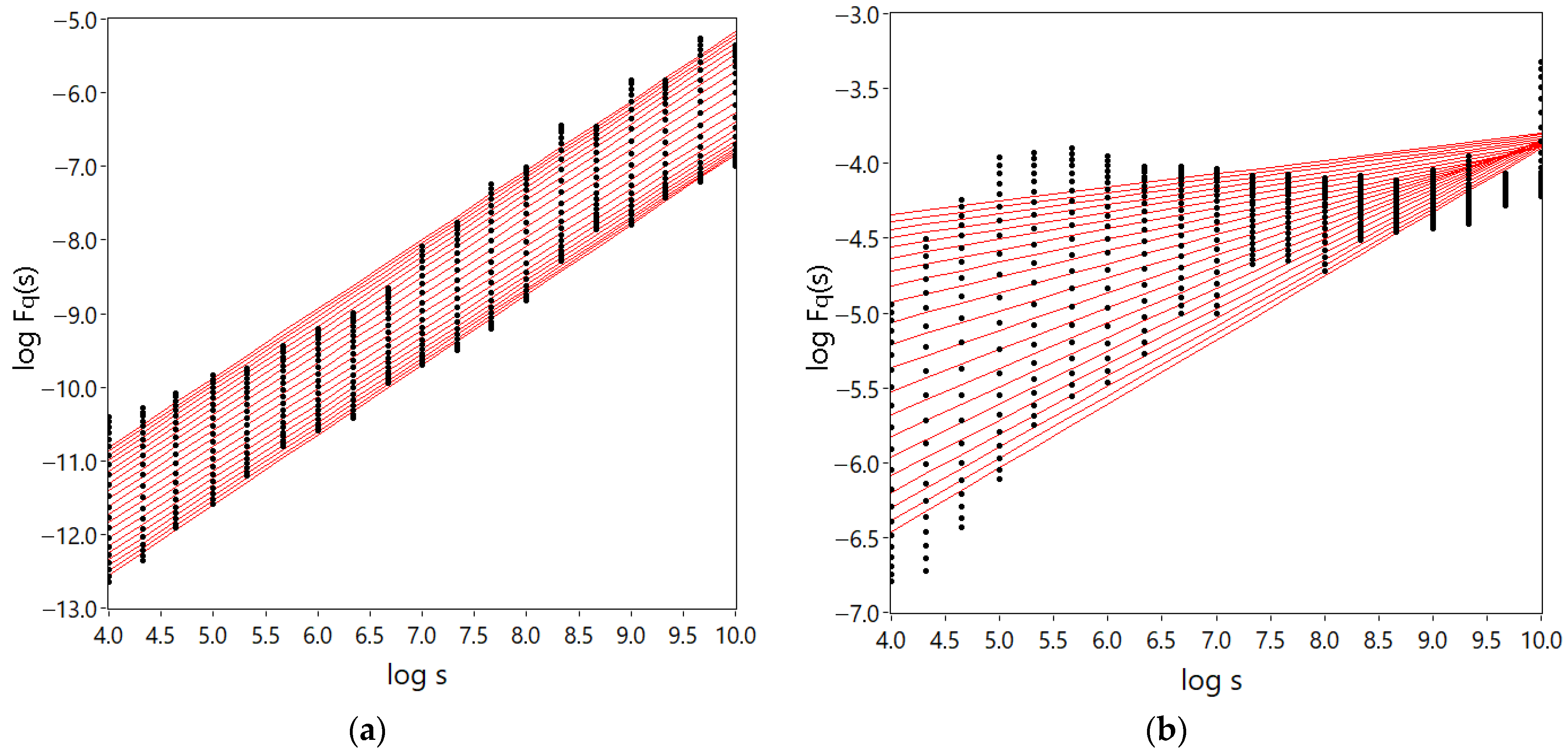
2.2. MF-DFA Algorithm

Based on the DFA, Kantelhardt J.U. et al. [35,36] proposed a multifractal analysis of fluctuations with a deterministic trend of nonstationary finite sequences. MF-DFA allows for obtaining a singular spectrum. Information about multifractal characteristics is extracted from it in order to quantify the complexity of the time series [33].
To evaluate the multifractality of a signal using the MF-DFA method, the following procedures must be performed.
  • The first three steps of the DFA algorithm are performed.
  • Averaging the values (2) deformed by an arbitrary parameter q, the values of the fluctuation function are found as follows:
F q s = 1 N s v = 1 N s F 2 ( v , s ) q / 2 1 / q ,
In the limit of q → 0, this expression should be used
F 0 s = e x p 1 2 N s v = 1 N s l n F 2 ( v , s ) ,
3.
Self-similar (scaling) behavior is represented by a power dependence:
F q s ~ s h q ,
If a number of experimental data correspond to a monofractal, then the generalized Hurst exponent h(q) in Equation (7) takes a single value h(q) = H. In the case of a multifractal, the index h becomes dependent on the deformation parameter q.
Within the framework of the standard fractal ideology, the transition from the Hurst exponent h(q) to the scaling exponent τ(q) is carried out as follows:
τ q = q h q 1 ,
Using Equation (8) and the Legendre transform, the multifractal spectrum f(α) is calculated as follows:
α = τ q ;   f ( α ) = q α τ q ,
where α —is the singularity strength or the Hölder exponent.

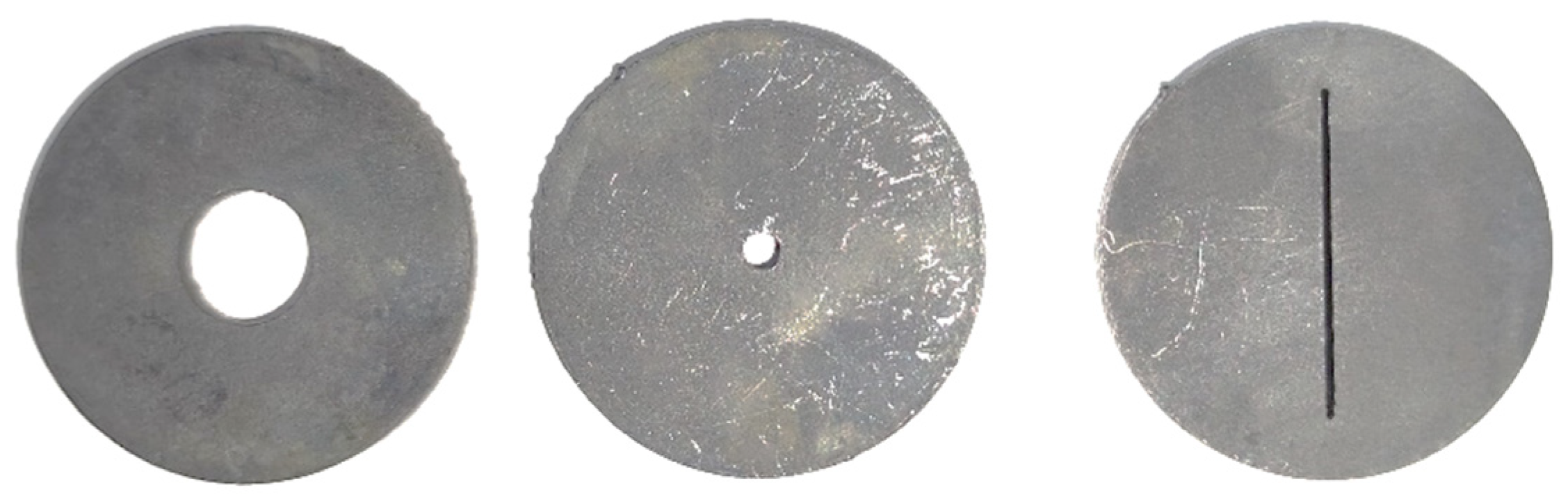
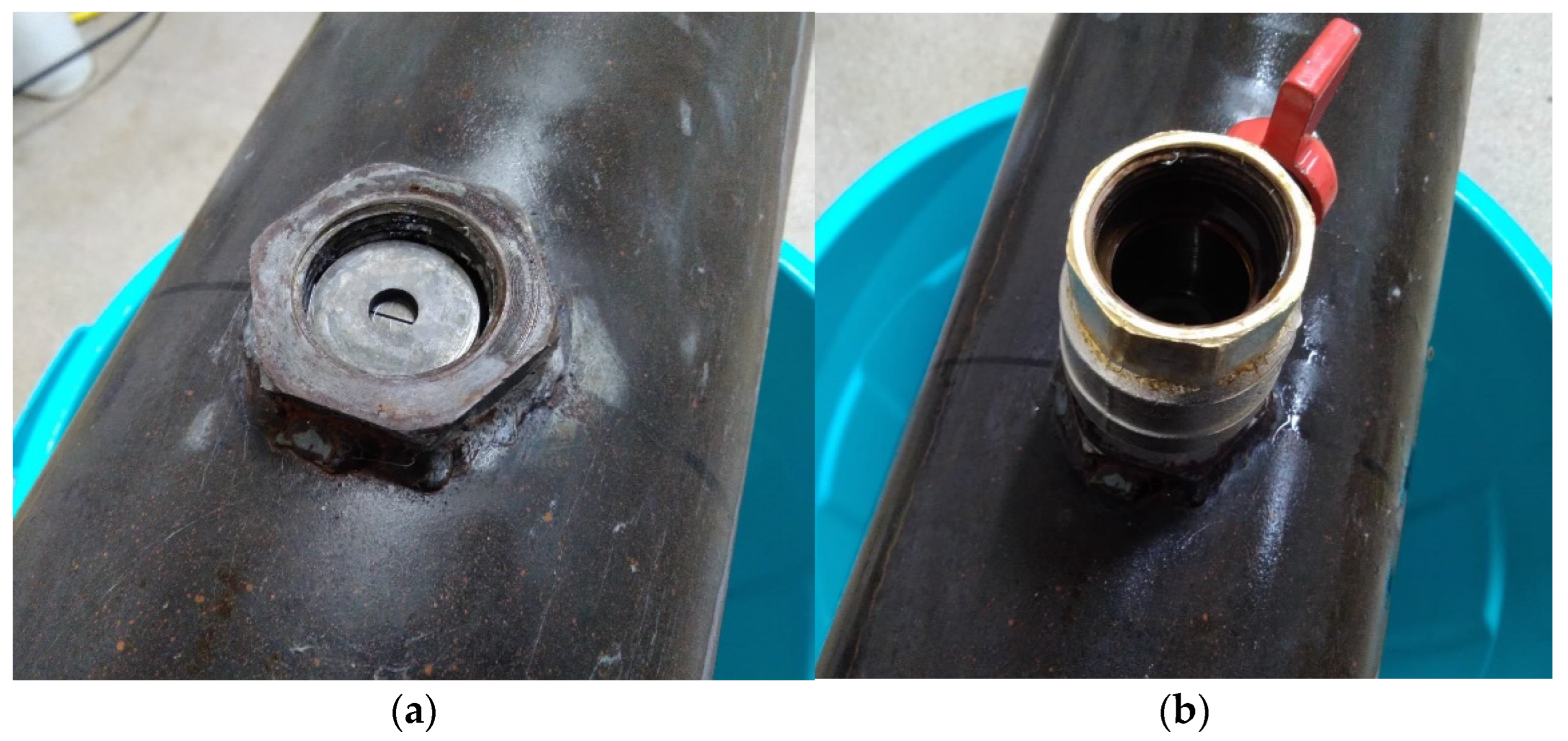
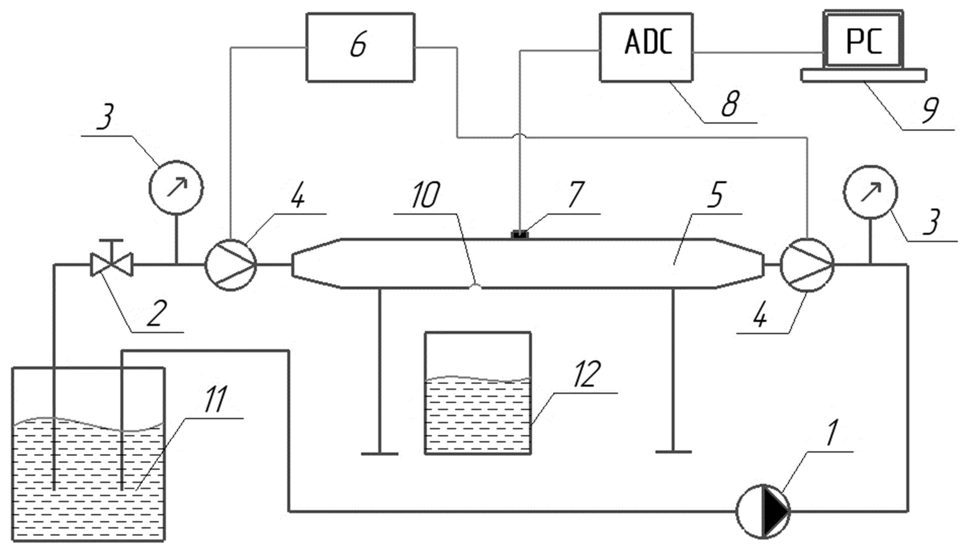
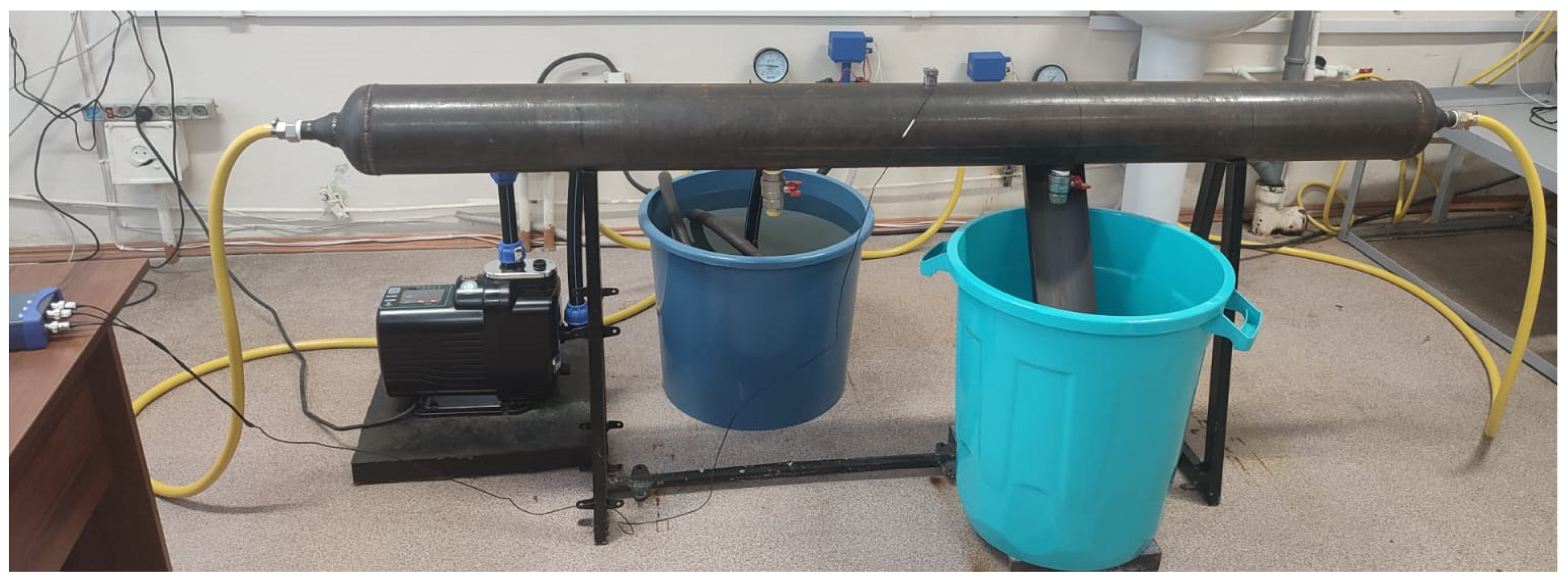
2.3. Description of the Experimental Stand

An experimental stand has been created to research the fractal characteristics of acoustic signals of pipelines with “slit” type defects.
Figure 1 shows the scheme of the experimental stand.
Water circulates in the closed circuit of the experimental stand. Pumping station 1 is equipped with a frequency-controlled drive and allows you to set different discharge pressure in the range from 1.5 to 4 bar. The hydraulic resistance of the system required for the operation of the pumping station was set by the cover of valve 2. Pressure and flow monitoring are provided by pressure gauges 3 and electromagnetic flow meters 4 installed at the ends of the pipe under study 5. The measuring unit 6 indicates the readings of the flow meters 4. Acoustic pipe signals were recorded by a three-component vibration acceleration sensor 7, which has the following characteristics: axial sensitivity of 1000 mV/g; and a natural frequency of 35 kHz. The analog-to-digital converter 8 has a sampling rate of 50 kHz. To eliminate noise from the impact of a jet of water, a plastic trough was installed in container 12.
Figure 2 shows a photo of the experimental stand.
In the course of the experiments, defects of the “slit” type pipeline with dimensions of 2 mm, 8 mm, and 20 mm were modeled. Steel discs were used for this (Figure 3):
  • With a slit 20 mm long and 0.5 mm wide.
  • A round hole with a diameter of 2 mm.
  • A round hole with a diameter of 8 mm.
To obtain slits with a length of 2 mm and 8 mm, discs with round holes of the appropriate diameter were placed on top of the disk with a gap. The discs were mounted on a fitting welded to the pipe and clamped with a ball valve, as shown in Figure 4.

3. Results and Discussion
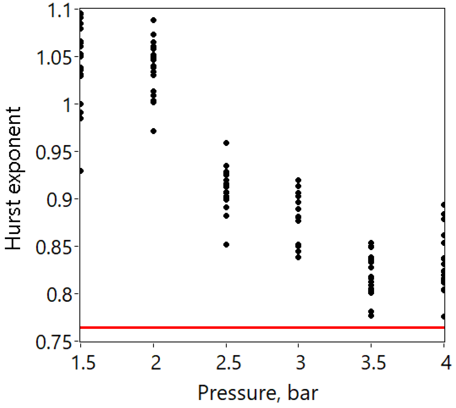
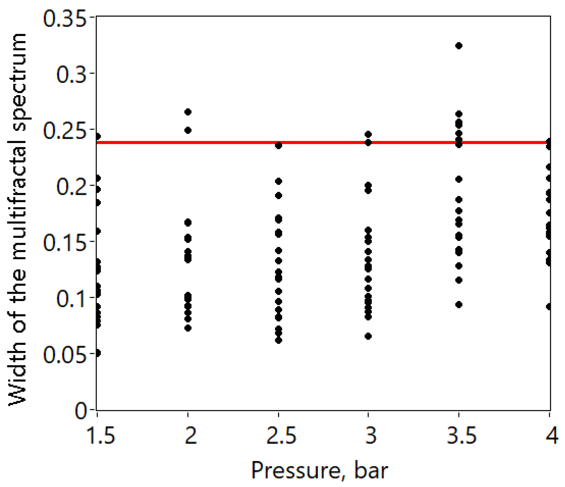
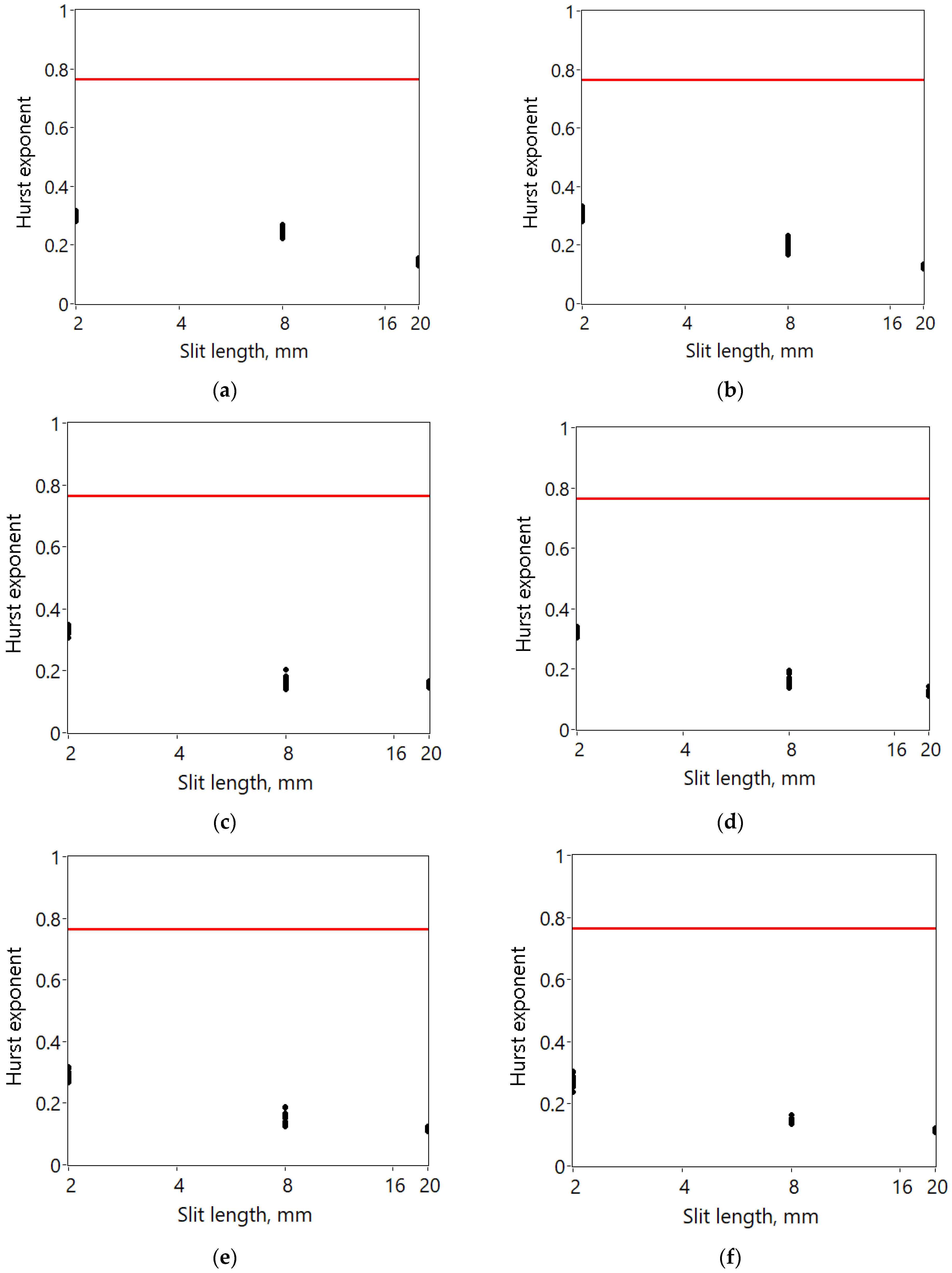
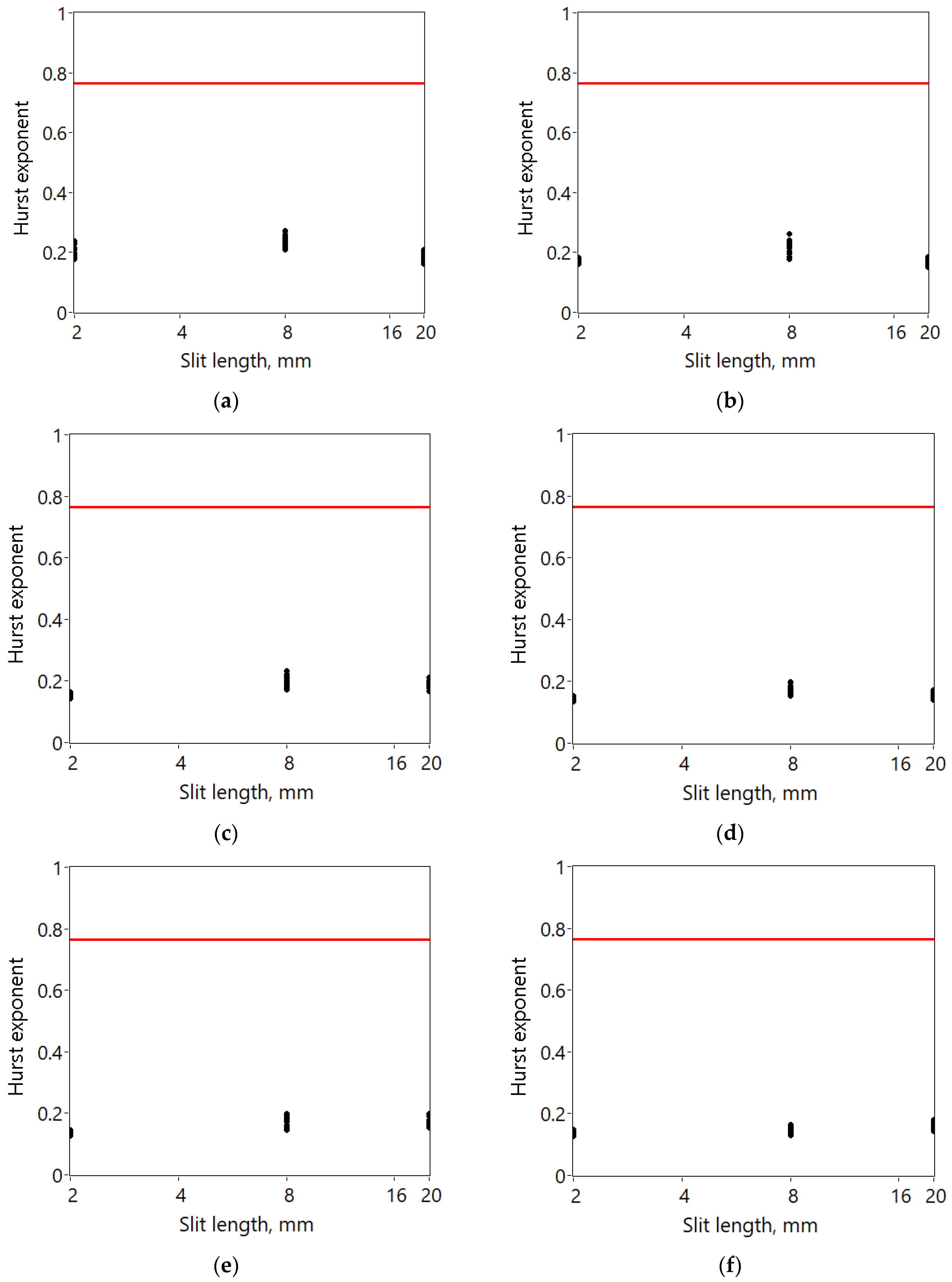
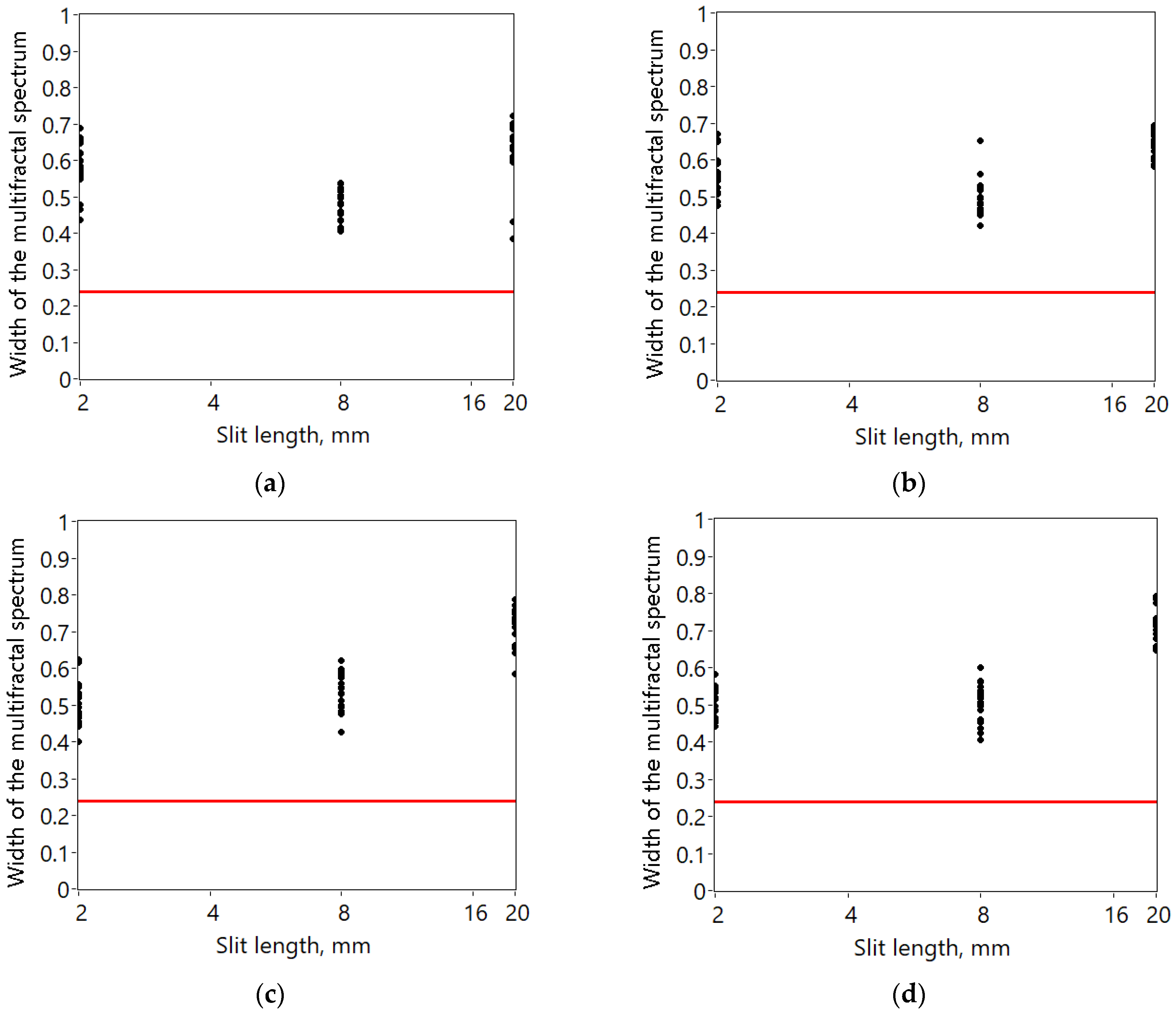
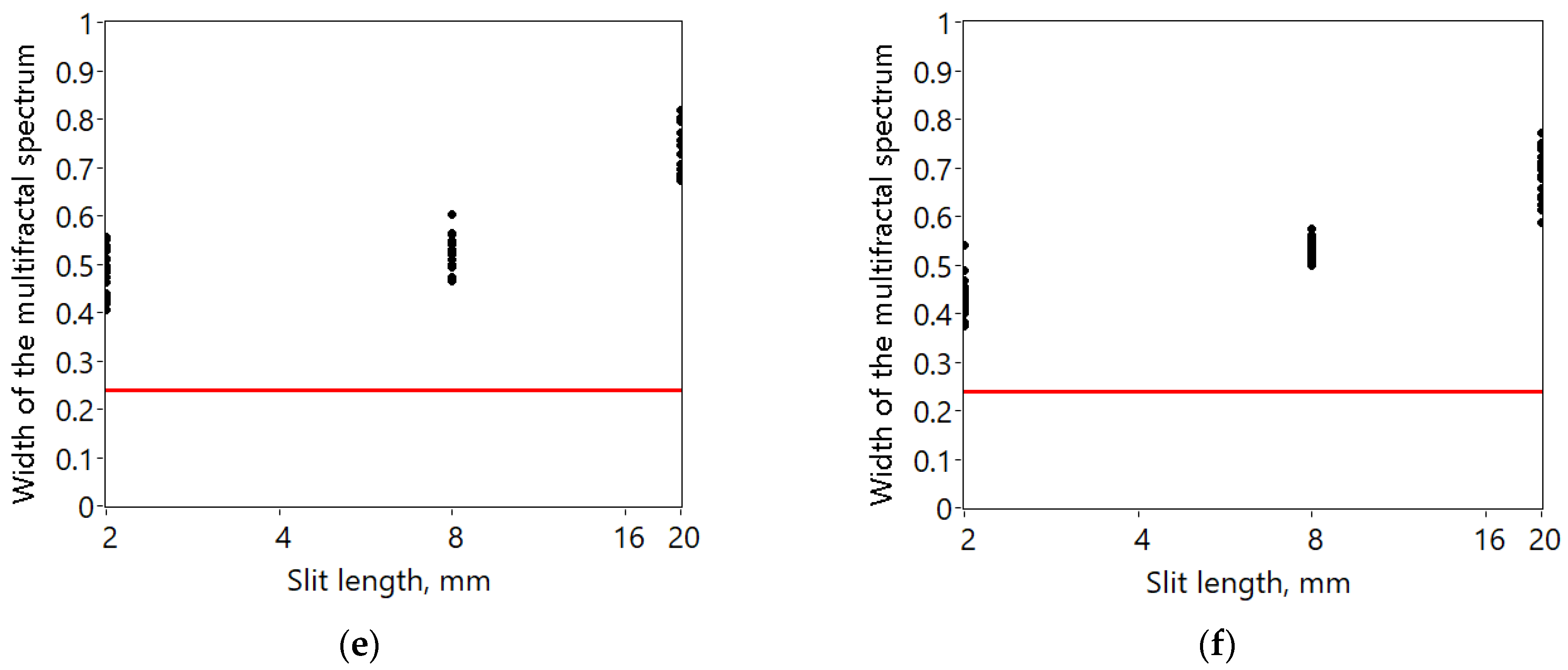
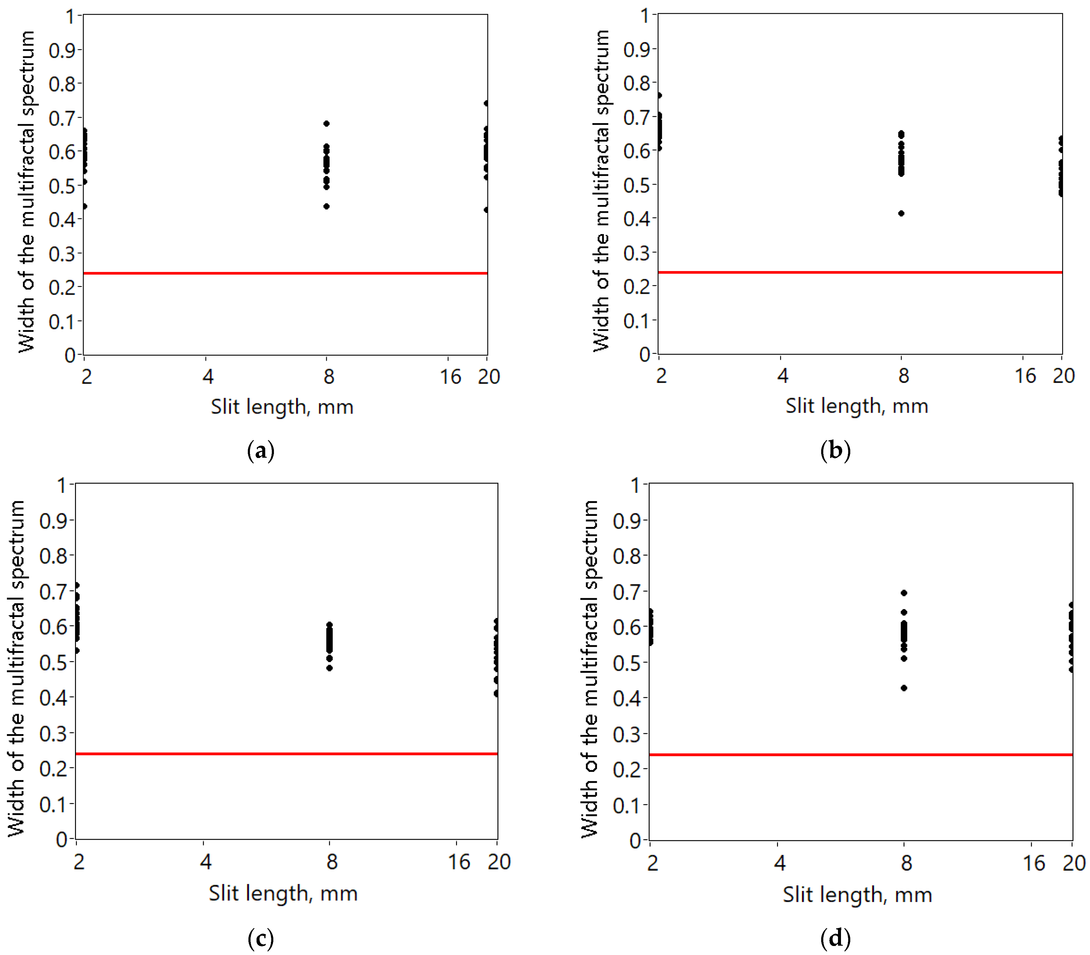
The experiment was conducted as follows. Discs were installed on the pipe, which simulated a leak. At the same time, the discs with a slit were alternately positioned both across and along the axis of the pipeline. By changing the rotation speed of the pump drive, a pressure in the range of 1.5–4 bar (in increments of 0.5 bar) was created in the pipeline. Acoustic signals were recorded at each pressure. The pipeline with a closed ball valve (see Figure 4) was assumed to be defect free.
The water consumption in a defect-free pipeline, depending on the pump discharge pressure, is shown in Table 1.
Table 2 shows the leakage costs depending on the size of the defect and the pump discharge pressure.
A software package has been written for signal analysis in the LabVIEW 2021 environment. Signals with a length of 20,000 samples were analyzed. The fluctuation function was calculated on signal segments (windows) with a length of s = 16 = 1024 samples. In step 3 of the DFA and MF-DFA algorithms, a polynomial of the first degree was used to approximate the segments of the y(i) profile.
The following approach was used to compare the results:
  • The median value of H ¯ was calculated for the signals of a defect-free pipeline;
  • The standard deviation S was calculated;
  • A confidence interval was constructed for a given level of significance α:
H ¯ ± S t ( 1 α / 2 , m 2 ) ,
where t (α, m)—α—is the quantile of the Student’s distribution with m degrees of freedom.
For each experiment, a sample of 20 acoustic signals was formed, which was used in the analysis of fractal characteristics.

3.1. Signal Analysis Using the DFA Method

According to the signals of the defect-free pipeline recorded at different pump discharge pressures, the lower limit of the confidence interval with a significance level of 0.05 was formed (Figure 5).
Figure 5 shows that as the pump discharge pressure increases, the Hurst exponent decreases. This effect can be explained by a change in the turbulence of the flow at local resistances. Thus, with an increase in water flow at the cover gate of valve 2 (Figure 1), turbulent pulsations of the water flow may increase, the acoustic noise of which is recorded by a vibration sensor.
For a defect-free pipeline, H > 0.5, which indicates the presence of long-term correlations in the acoustic signal (large oscillation amplitudes follow large ones, small ones follow small ones).
Figure 6 and Figure 7 show a comparison with the lower limit of the confidence interval of the values of the Hurst exponent of acoustic signals of a pipeline with a transverse and longitudinal location of defects.
With the appearance of a leak in the pipeline, the Hurst exponent decreases (H < 0.5), and the acoustic signal becomes anti-correlated (large and small amplitudes alternate in the signal). This is due to the appearance of chaotic pressure pulsations of water flowing turbulently through a through slit in the pipe wall. Such vibrations lead to the appearance of elastic waves in the fluid itself and in the walls of the pipe, which are recorded by a vibration sensor.
It can be seen from Figure 6 and Figure 7 that the values of the Hurst exponent of the acoustic signals of the pipeline, with the considered defects, go beyond the boundaries of the confidence interval.

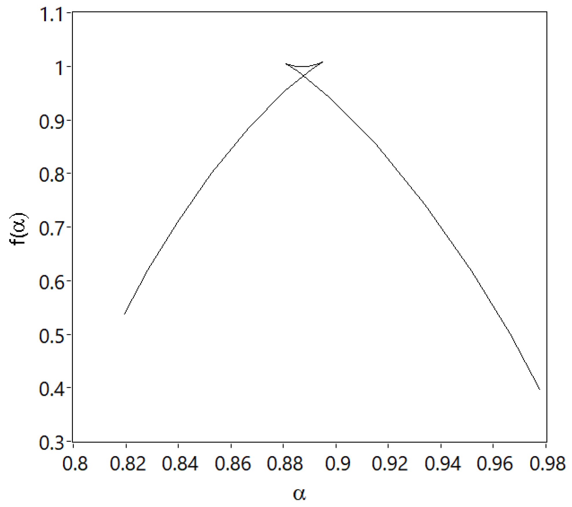
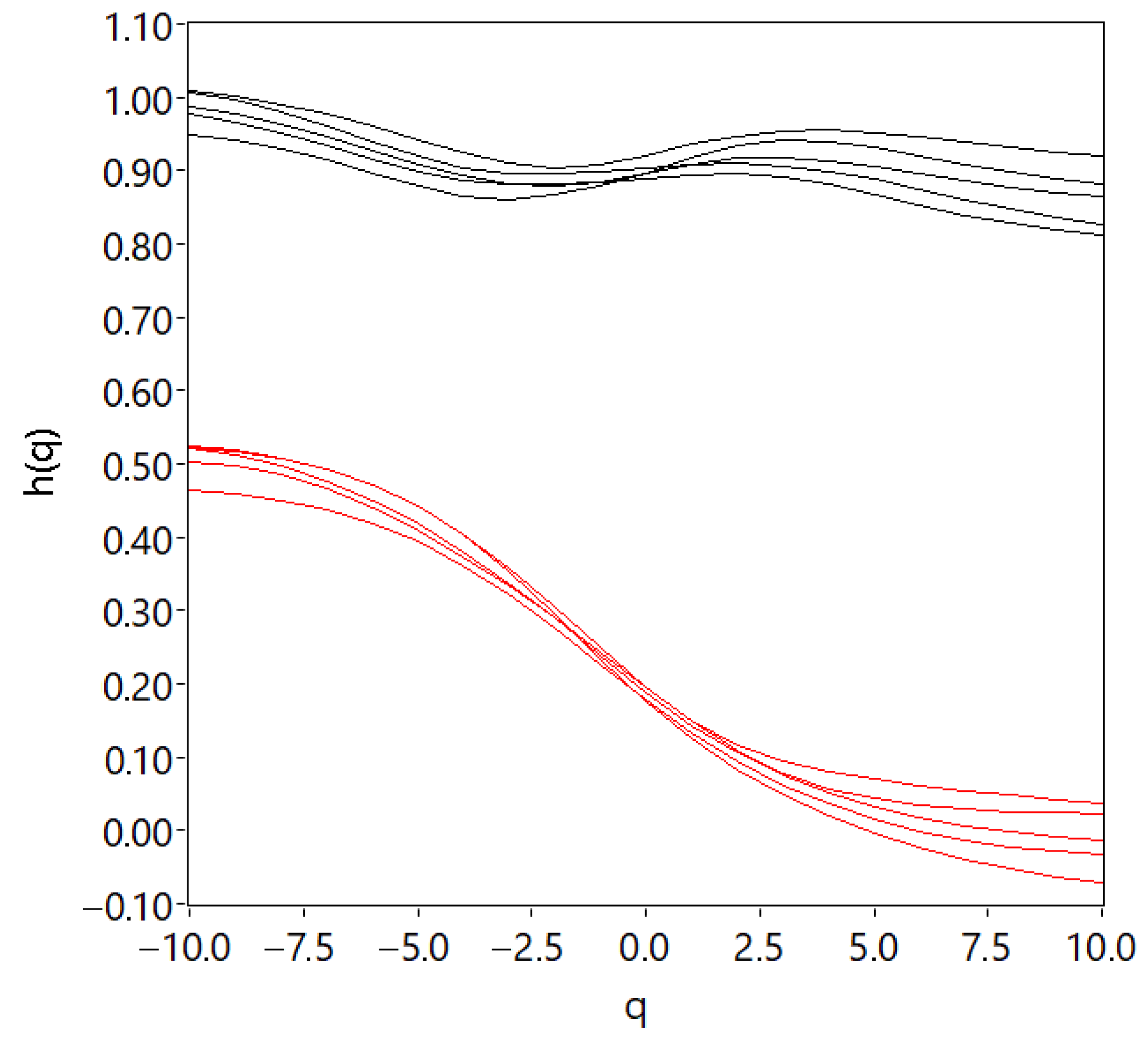
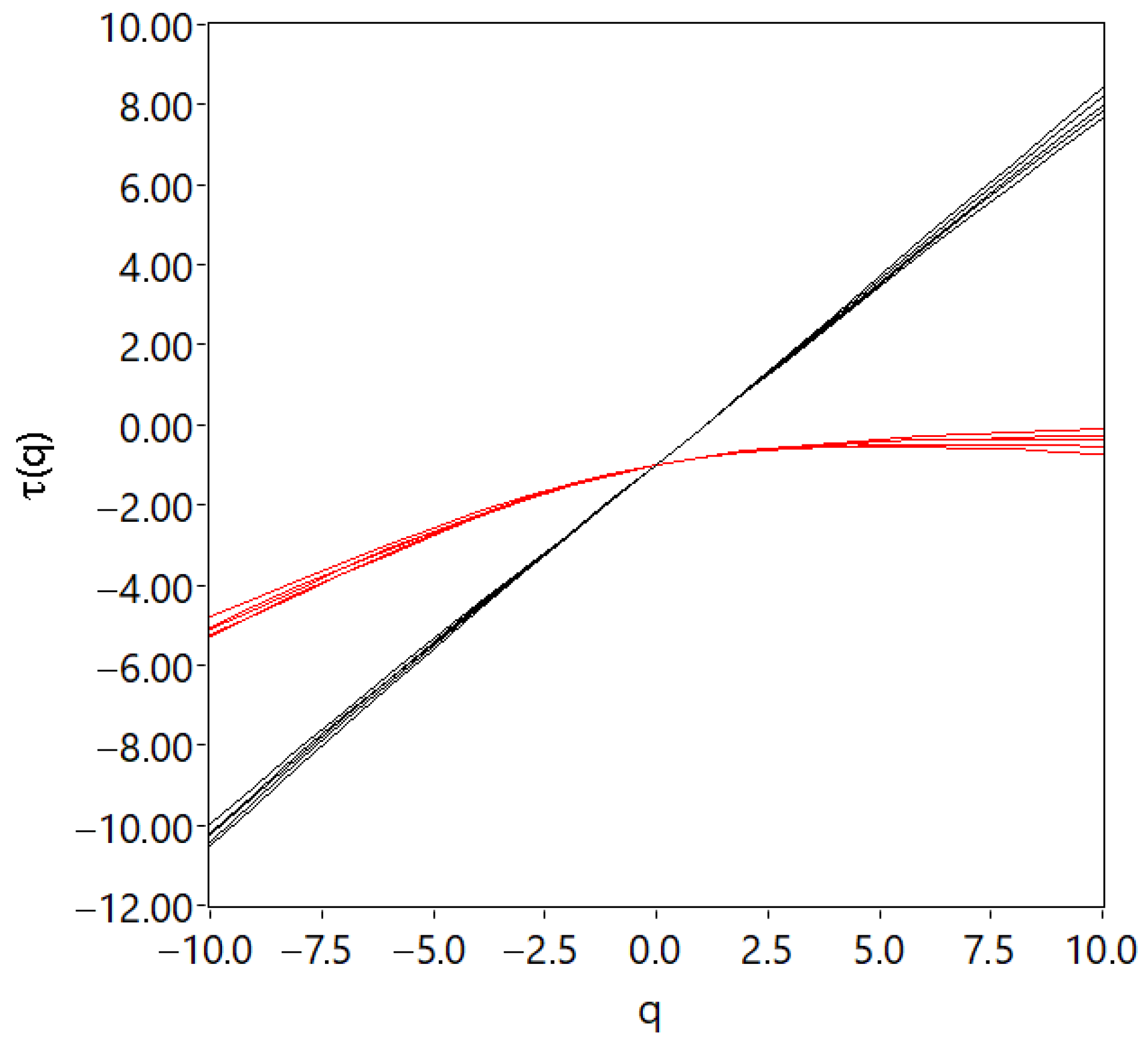
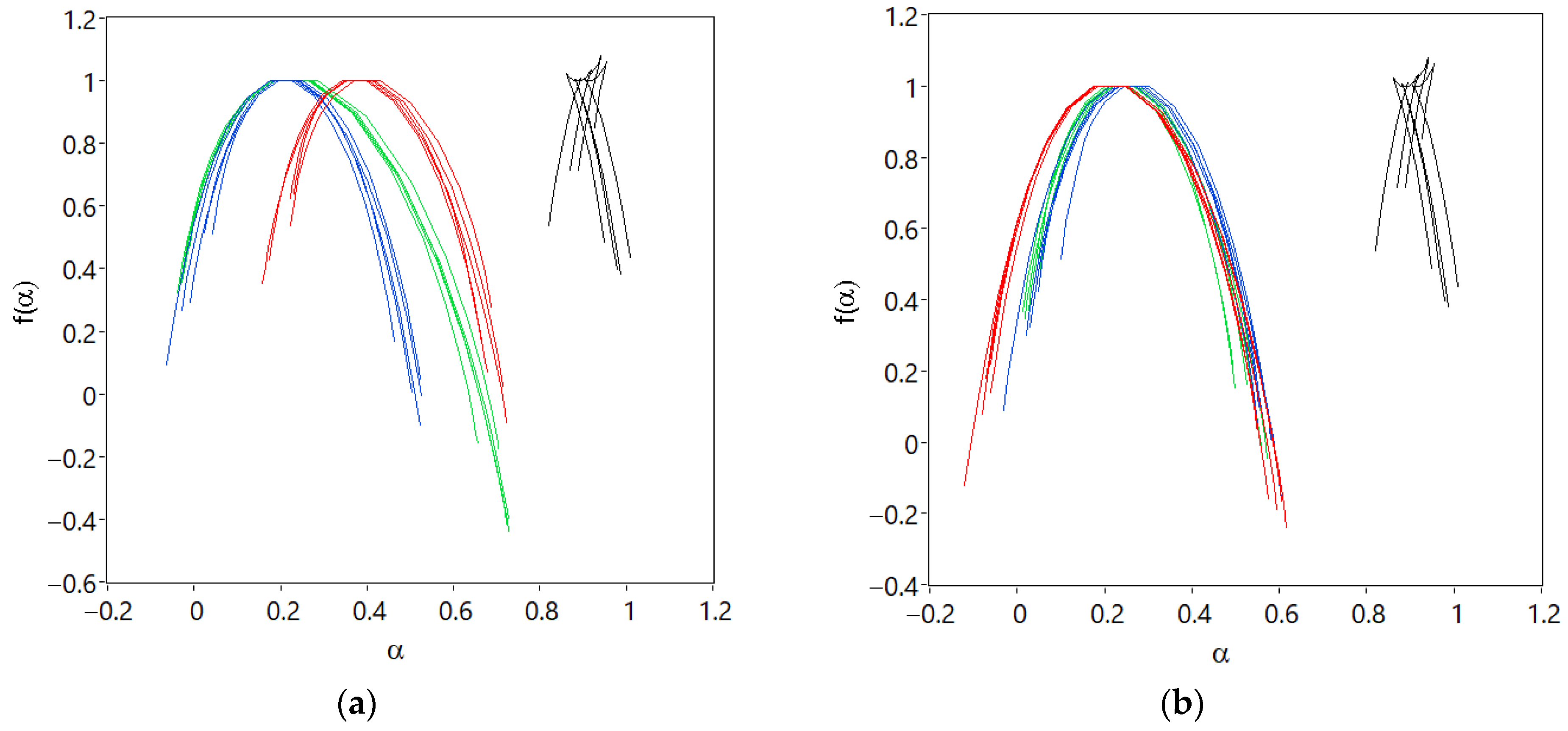
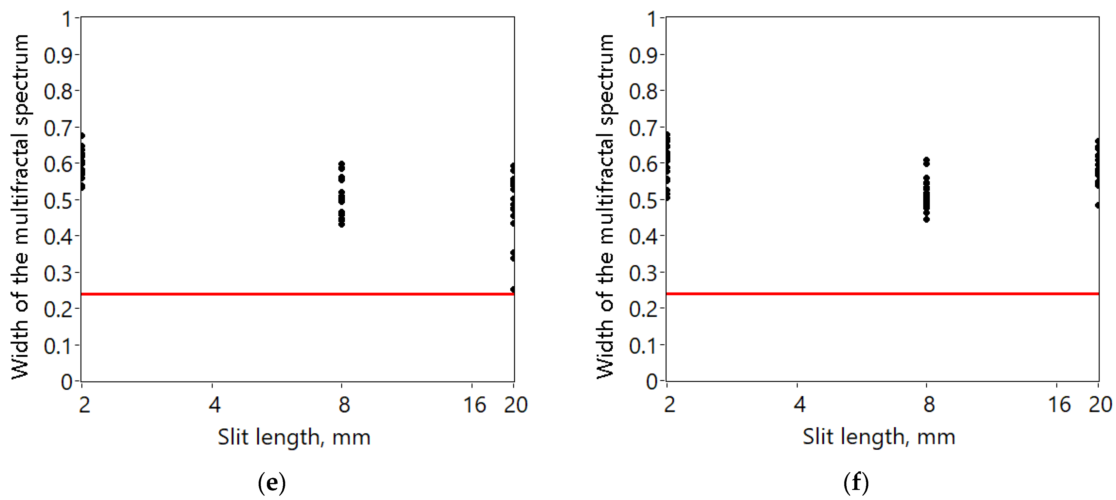
3.2. Signal Analysis Using the MF-DFA Method

The multifractal characteristics of acoustic signals were analyzed. The signals of a pipeline without defects and a pipeline with a transverse defect of 8 mm at the same pressure of 2.5 bar were compared.
The change in the fluctuation functions Fq(s) depends on the scale s and the deformation parameter q (Figure 8). It can be seen that the slopes of the regression lines for pipeline signals with leakage depend on the value of the parameter q, which is a characteristic feature of multifractal processes.
The generalized Hurst exponent h(q) and the scaling exponent τ(q) also indicate the multifractal features of the acoustic signals of the defective pipeline (Figure 9 and Figure 10).
According to the graph of the generalized Hurst exponent (Figure 9), it can be seen that the acoustic signals of a defective pipeline are characterized by a pronounced nonlinear dependence h(q). It should be noted that the signals of a defect-free pipeline at values q = ±5 have a slight nonlinearity.
For the signals of a defect-free pipeline, a rectilinear dependence of τ(q), characteristic of monofractal objects, is observed. For pipeline signals with leakage, the function τ(q) bends.
The structure of a self-similar object is most vividly represented by the shape of the multifractal spectrum f(α).
The multifractal spectrum characteristic of all acoustic signals of a defect-free pipeline is shown in Figure 11. It can be seen that its shape differs from the parabolic one, which is typical for multifractal objects. Similar forms of multifractal spectrum are presented in the works of other authors [37,38,39].
With the appearance of a leak in the pipeline, the width of the multifractal spectrum increases, they acquire a parabolic shape and shift along the axis of the abscissa (Figure 12). An increase in the width of the spectrum indicates a higher degree of multifractality of the defective pipeline signals.
To quantitatively compare the multifractal spectrum of acoustic signals, their width was calculated as follows:
α = α m a x α m i n ,
According to the acoustic signals of the defect-free pipe obtained at different pump discharge pressures, an upper bound of the confidence interval with a significance level of 0.05 was formed (Figure 13).
A comparison of the width of the multifractal spectrum of a defective pipeline with the upper limit of the confidence interval is shown in Figure 14 and Figure 15. It can be seen from these figures that the values of all acoustic signals of the leaky pipeline go beyond the boundaries of the confidence interval.
Since the acoustic signals of the pipeline contain fractal noise, it is not always possible to investigate them using traditional methods of covariance and spectral analysis. Therefore, filtration of the noise component of signals is used in pipeline leak monitoring systems [13,40]. However, the noise being removed carries useful diagnostic information that can be extracted using fractal analysis methods. The results obtained in this work showed a high reliability of leak detection by DFA and MF-DFA methods.

4. Conclusions

As a result of experimental studies, it was found that the occurrence of leakage leads to the occurrence of anti-correlated oscillations with multifractal properties in the pipeline. Large and small amplitudes alternate in the acoustic signal of a defective pipeline, and there is a wide variation in the Hölder exponent.
The received acoustic signals of the defect-free pipeline are correlated, which are similar in structure to monofractals.
The Hurst exponent of signals of a defect-free pipeline is H = 0.92 ± 0.16, and the width of the multifractal spectrum is Δα = 0.15 ± 0.09. With the appearance of leakage, the Hurst exponent decreases, and the width of the multifractal spectrum increases.
The analysis of acoustic signals by DFA and MF-DFA methods makes it possible to reliably determine the leakage. The Hurst exponent and the width of the multifractal spectrum can serve as indicators of the occurrence of leaks in pipelines.
However, the fractal characteristics of the acoustic signal may be influenced by turbulent pulsations of the fluid flow that occur at local resistances (for example, closed valves, and sharp constrictions). In this regard, it is necessary to determine the reference level of the Hurst exponent and the width of the multifractal spectrum when changing the parameters of the pipeline system.

Author Contributions

Conceptualization, A.Z. and S.Z.; software A.Z.; investigation, S.Z., E.I., I.K. and R.A.; validation, Y.V.; writing—original draft preparation, S.Z. and E.I.; writing—review and editing, A.Z.; data curation, I.K. and R.A. All authors have read and agreed to the published version of the manuscript.

Funding

This research was funded by the Russian Science Foundation grant No. 22-79-10045, https://rscf.ru/en/project/22-79-10045/ (accessed date 19 February 2024).

Data Availability Statement

Not applicable.

Conflicts of Interest

The authors declare no conflicts of interest.

References

  1. Yao, L.; Zhang, Y.; He, T.; Luo, H. Natural gas pipeline leak detection based on acoustic signal analysis and feature reconstruction. Appl. Energy 2023, 352, 121975. [Google Scholar] [CrossRef]
  2. Sun, L.; Zhu, J.; Tan, J.; Li, X.; Li, R.; Deng, H.; Zhang, X.; Liu, B.; Zhu, X. Deep learning-assisted automated sewage pipe defect detection for urban water environment management. Sci. Total Env. 2023, 882, 163562. [Google Scholar] [CrossRef] [PubMed]
  3. Meijer, D.; Scholten, L.; Clemens, F.; Knobbe, A. A defect classification methodology for sewer image sets with convolutional neural networks. Autom. Constr. 2019, 104, 281–298. [Google Scholar] [CrossRef]
  4. Li, J.; Zheng, Q.; Qian, Z.; Yang, X. A novel location algorithm for pipeline leakage based on the attenuation of negative pressure wave. Process Saf. Environ. Prot. 2019, 123, 309–316. [Google Scholar] [CrossRef]
  5. Lu, Q.; Li, Q.; Hu, L.; Huang, L. An effective Low-Contrast SF₆ gas leakage detection method for infrared imaging. IEEE Trans. Instrum. Meas. 2021, 70, 5009009. [Google Scholar] [CrossRef]
  6. Lu, H.; Iseley, T.; Behbahani, S.; Fu, L. Leakage detection techniques for oil and gas pipelines: State-of-the-art. Tunnell. Undergr. Space Technol. 2020, 98, 103249. [Google Scholar] [CrossRef]
  7. Fan, H.; Tariq, S.; Zayed, T. Acoustic leak detection approaches for water pipelines. Autom. Constr. 2022, 138, 104226. [Google Scholar] [CrossRef]
  8. Yu, T.; Chen, X.; Yan, W.; Xu, Z.; Ye, M. Leak detection in water distribution systems by classifying vibration signals. Mech. Syst. Signal Process. 2023, 185, 109810. [Google Scholar] [CrossRef]
  9. Hunaidi, O.; Chu, W.T. Acoustical characteristics of leak signals in plastic water distribution pipes. Appl. Acoust. 1999, 58, 235–254. [Google Scholar] [CrossRef]
  10. Zagretdinov, A.R.; Kazakov, R.B.; Mukatdarov, A.A. Control the tightness of the pipeline valve shutter according to the change in the Hurst exponent of vibroacoustic signals. E3S Web Conf. 2019, 124, 03005. [Google Scholar] [CrossRef]
  11. Krainova, L.N.; Munitsyn, A.I. Prostranstvennye nelinejnye kolebaniya truboprovoda pri garmonicheskom vozbuzhdenii [Three-dimensional non-linear oscillations of the pipeline at harmonic excitation]. Mashinostroenie I Inzhenernoe Obraz. Mech. Eng. Eng. Educ. 2010, 2, 46–51. (In Russian) [Google Scholar]
  12. Bykerk, L.; Valls Miro, J. Vibro-Acoustic Distributed Sensing for Large-Scale Data-Driven Leak Detection on Urban Distribution Mains. Sensors 2022, 22, 6897. [Google Scholar] [CrossRef] [PubMed]
  13. Wang, W.; Gao, Y. Pipeline leak detection method based on acoustic-pressure information fusion. Measurement 2023, 212, 112691. [Google Scholar] [CrossRef]
  14. Luo, P.; Yang, W.; Sun, M.; Shen, G.; Zhang, S. Experimental study on acoustic signal characteristic analysis and time delay estimation of pipeline leakage in boilers. Meas. Sci. Technol. 2024, 35, 035105. [Google Scholar] [CrossRef]
  15. Zeng, W.; Do, N.; Lambert, M.; Gong, J.; Cazzolato, B.; Stephen, M. Linear phase detector for detecting multiple leaks in water pipes. Appl. Acoust. 2023, 202, 109152. [Google Scholar] [CrossRef]
  16. Wang, W.; Sun, H.; Guo, J.; Lao, L.; Wu, S.; Zhang, J. Experimental study on water pipeline leak using In-Pipe acoustic signal analysis and artificial neural network prediction. Measurement 2021, 186, 110094. [Google Scholar] [CrossRef]
  17. Duan, Q.; An, J.; Mao, H.; Liang, D.; Li, H.; Wang, S.; Huang, C. Review about the Application of Fractal Theory in the Research of Packaging Materials. Materials 2021, 14, 860. [Google Scholar] [CrossRef] [PubMed]
  18. Dimri, V.P.; Ganguli, S.S. Fractal Theory and Its Implication for Acquisition, Processing and Interpretation (API) of Geophysical Investigation: A Review. J. Geol. Soc. India 2019, 93, 142–152. [Google Scholar] [CrossRef]
  19. Tang, S.W.; He, Q.; Xiao, S.Y.; Huang, X.Q.; Zhou, L. Fractal Plasmonic Metamaterials: Physics and Applications. Nanotechnol. Rev. 2015, 4, 277–288. [Google Scholar] [CrossRef]
  20. Babanin, O.; Bulba, V. Designing the technology of express diagnostics of electric train’s traction drive by means of fractal analysis. East.-Eur. J. Enterp. Technol. 2016, 4, 45–54. [Google Scholar] [CrossRef]
  21. Li, Q.; Liang, S.Y. Degradation trend prognostics for rolling bearing using improved R/S statistic model and fractional brownian motion approach. IEEE Access 2017, 6, 21103–21114. [Google Scholar] [CrossRef]
  22. Datta, D.; Sathish, S. Application of fractals to detect breast cancer. J. Phys. Conf. Ser. 2019, 1377, 012030. [Google Scholar] [CrossRef]
  23. Hart, M.G.; Romero-Garcia, R.; Price, S.J.; Suckling, J. Global effects of focal brain tumors on functional complexity and network robustness: A prospective cohort study. Clin. Neurosurg. 2019, 84, 1201–1213. [Google Scholar] [CrossRef] [PubMed]
  24. Dona, O.; Hall, G.B.; Noseworthy, M.D. Temporal fractal analysis of the rs-BOLD signal identifies brain abnormalities in autism spectrum disorder. PLoS ONE 2017, 12, e0190081. [Google Scholar] [CrossRef] [PubMed]
  25. Chandrasekaran, S.; Poomalai, S.; Saminathan, B.; Suthanthiravel, S.; Sundaram, K.; Hakkim, F.F.A. An investigation on the relationship between the hurst exponent and the predictability of a rainfall time series. Meteorol. Appl. 2019, 26, 511–519. [Google Scholar] [CrossRef]
  26. Jiang, Z.-Q.; Xie, W.-J.; Zhou, W.-X.; Sornette, D. Multifractal Analysis of Financial Markets: A Review. Rep. Prog. Phys. 2019, 82, 125901. [Google Scholar] [CrossRef] [PubMed]
  27. Jeldres, R.I.; Fawell, P.D.; Florio, B.J. Population Balance Modelling to Describe the Particle Aggregation Process: A review. Powder Technol. 2018, 326, 190–207. [Google Scholar] [CrossRef]
  28. Xie, X.; Li, S.; Guo, J. Study on Multiple Fractal Analysis and Response Characteristics of Acoustic Emission Signals from Goaf Rock Bodies. Sensors 2022, 22, 2746. [Google Scholar] [CrossRef] [PubMed]
  29. Akhmetkhanov, R. The Patterns of the Power Spectral Density Distribution of Fractal and Multifractal Processes. J. Mach. Manuf. Reliab. 2018, 47, 235–240. [Google Scholar] [CrossRef]
  30. Li, H.; Qiao, Y.; Shen, R.; He, M. Electromagnetic radiation signal monitoring and multi-fractal analysis during uniaxial compression of water-bearing sandstone. Measurement 2022, 196, 111245. [Google Scholar] [CrossRef]
  31. Porziani, S.; Augugliaro, G.; Brini, F.; Brutti, C.; Chiappa, A.; Groth, C.; Mennuti, C.; Quaresima, P.; Salvini, P.; Zanini, A.; et al. Structural integrity assessment of pressure equipment by Acoustic Emission and data fractal analysis. Procedia Struct. Integr. 2020, 25, 246–253. [Google Scholar] [CrossRef]
  32. Zagretdinov, A.; Ziganshin, S.; Vankov, Y.; Izmailova, E.; Kondratiev, A. Determination of Pipeline Leaks Based on the Analysis the Hurst Exponent of Acoustic Signals. Water 2022, 14, 3190. [Google Scholar] [CrossRef]
  33. Alam, A.; Nikolopoulos, D.; Wang, N. Fractal Patterns in Groundwater Radon Disturbances Prior to the Great 7.9 Mw Wenchuan Earthquake, China. Geosciences 2023, 13, 268. [Google Scholar] [CrossRef]
  34. Peng, C.K.; Buldyrev, S.V.; Havlin, S.; Simons, M.; Stanley, H.E.; Goldberger, A.L. Mosaic Organization of DNA Nucleotides. Phys. Rev. E 1994, 49, 1685–1689. [Google Scholar] [CrossRef] [PubMed]
  35. Kantelhardt, J.W.; Zschiegner, S.A.; Koscielny-Bunde, E.; Havlin, S.; Bunde, A.; Stanley, H.E. Multifractal Detrended Fluctuation Analysis of Nonstationary Time Series. Phys. A Stat. Mech. Appl. 2002, 316, 87–114. [Google Scholar] [CrossRef]
  36. Ihlen, E.A. Introduction to Multifractal Detrended Fluctuation Analysis in Matlab. Front. Physiol. 2012, 3, 141. [Google Scholar] [CrossRef] [PubMed]
  37. Kojić, M.; Mitić, P.; Dimovski, M.; Minović, J. Multivariate Multifractal Detrending Moving Average Analysis of Air Pollutants. Mathematics 2021, 9, 711. [Google Scholar] [CrossRef]
  38. Puchalski, A.; Komorska, I. Data-driven monitoring of the gearbox using multifractal analysis and machine learning methods. MATEC Web Conf. 2019, 252, 06006. [Google Scholar] [CrossRef]
  39. Hong, L.; Shu, W.; Chao, A.C. Recurrence Interval Analysis on Electricity Consumption of an Office Building in China. Sustainability 2018, 10, 306. [Google Scholar] [CrossRef]
  40. Henrie, M.; Carpenter, P.; Nicholas, R.E. Statistical Processing and Leak Detection. In Pipeline Leak Detection Handbook; Gulf Professional Publishing: Houston, TX, USA, 2016; pp. 91–114. [Google Scholar] [CrossRef]
Figure 1. The scheme of the experimental stand: 1—pumping station LEO MAC550; 2—valve; 3—manometer; 4—electromagnetic flow meter Vzljot; 5—steel pipe (outer diameter 159 mm, wall thickness 6 mm, length 2 m); 6—measuring unit Vzljot; 7—vibration acceleration sensor AP2038P-1000; 8—analog-to-digital converter Zetlab ZET 030; 9—PC; 10—defect; 11—water storage capacity; 12—drain container.
Fractalfract 08 00213 g001
Figure 2. Photo of the experimental stand.
Fractalfract 08 00213 g002
Figure 3. Steel discs.
Fractalfract 08 00213 g003
Figure 4. The method of mounting discs on the pipe: (a) laying discs; (b) installing a ball valve on top of discs.
Fractalfract 08 00213 g004
Figure 5. The values of the Hurst exponent (black points) of acoustic signals of a defect-free pipeline and the lower limit of the confidence interval (red line).
Fractalfract 08 00213 g005
Figure 6. The values of the Hurst exponent (black points) of acoustic signals of a pipeline with a transverse arrangement of defects at different pump discharge pressures: (a) 1.5 bar; (b) 2 bar; (c) 2.5 bar; (d) 3 bar; (e) 3.5 bar; (f) 4 bar. The red line shows the lower limit of the confidence interval.
Fractalfract 08 00213 g006
Figure 7. The values of the Hurst exponent (black points) of acoustic signals of a pipeline with longitudinal defects at different pump discharge pressures: (a) 1.5 bar; (b) 2 bar; (c) 2.5 bar; (d) 3 bar; (e) 3.5 bar; (f) 4 bar. The red line shows the lower limit of the confidence interval.
Fractalfract 08 00213 g007
Figure 8. The values of the function Fq(s) (black points) depending on the scale of s on a logarithmic scale for different parameters q and the regression line (red): (a) for the signal of a defect-free pipeline; (b) for the signal of a pipeline with a leak.
Fractalfract 08 00213 g008
Figure 9. Graphs of the generalized Hurst exponent: black lines—for signals of a defect-free pipeline, red lines—for signals of a pipeline with a leak.
Fractalfract 08 00213 g009
Figure 10. Graphs of the scaling exponent τ(q): black lines—for signals of a defect-free pipeline, red lines—for signals of a pipeline with a leak.
Fractalfract 08 00213 g010
Figure 11. The multifractal spectrum of the acoustic signal of a defect-free pipeline.
Fractalfract 08 00213 g011
Figure 12. The multifractal spectrum of acoustic signals of pipeline at a pump discharge pressure of 2.5 bar: (a) with a transverse defect location; (b) with a longitudinal defect location; black line—for a defect-free pipeline; red line—for a pipeline with a defect of 2 mm; blue line—for a pipeline with a defect of 8 mm; green line—for a pipeline with a defect of 20 mm.
Fractalfract 08 00213 g012
Figure 13. The values of the width of the multifractal spectrum (black points) of acoustic signals of a defect-free pipeline and the upper limit of the confidence interval (red line).
Fractalfract 08 00213 g013
Figure 14. The values of the width of the multifractal signal spectrum (black points) of a pipeline with a transverse arrangement of defects at different pump discharge pressures: (a) 1.5 bar; (b) 2 bar; (c) 2.5 bar; (d) 3 bar; (e) 3.5 bar; (f) 4 bar. The red line shows the upper limit of the confidence interval.
Fractalfract 08 00213 g014aFractalfract 08 00213 g014b
Figure 15. The values of the width of the multifractal spectrum (black points) of pipeline signals with longitudinal defects at different pump discharge pressures: (a) 1.5 bar; (b) 2 bar; (c) 2.5 bar; (d) 3 bar; (e) 3.5 bar; (f) 4 bar. The red line shows the upper limit of the confidence interval.
Fractalfract 08 00213 g015aFractalfract 08 00213 g015b
Table 1. The operating characteristic of the pump obtained on a defect-free pipeline.
Pump Discharge Pressure, BarPump Capacity, L/min
1.57.02
28.16
2.59.72
310.35
3.511.1
411.85
Table 2. Leakage rate.
Slit Length, mmPump Discharge Pressure, BarLeakage Rate, L/min
21.50.9
21.14
2.51.32
31.38
3.51.5
41.53
81.53.3
23.75
2.54.26
34.62
3.55.07
45.43
201.57.95
29.36
2.510.6
311.46
3.512.27
413.02
Disclaimer/Publisher’s Note: The statements, opinions and data contained in all publications are solely those of the individual author(s) and contributor(s) and not of MDPI and/or the editor(s). MDPI and/or the editor(s) disclaim responsibility for any injury to people or property resulting from any ideas, methods, instructions or products referred to in the content.

