Abstract
This research project focuses on developing a mathematical model that allows us to understand the behavior of the balancing loops in system dynamics in greater detail and precision. Currently, simulations give us an understanding of the behavior of these loops, but under the premise of an ideal scenario. In practice, however, accurate models often operate with varying efficiencies due to various irregularities and particularities. This discrepancy is the primary motivation behind our research proposal, which seeks to provide a more realistic understanding of the behavior of the loops, including their different levels of efficiency. To achieve this goal, we propose the introduction of fractional calculus in system dynamics models, focusing specifically on the balancing loops. This innovative approach offers a new perspective on the state of the art, offering new possibilities for understanding and optimizing complex systems.
1. Introduction
System dynamics (SD), as a modeling and simulation discipline, has emerged as a fundamental tool in solving complex and dynamic problems across various fields from business management to environmental science. These models, grounded in systems theory and computer simulation, empower researchers and professionals to comprehend and analyze the behavior of dynamic systems over time [1]. The primary objective of this technique is to capture causal relationships and mechanisms underlying observed phenomena, providing an invaluable perspective for decision-making and addressing complex challenges in a world characterized by interconnection and interdependence [2].
System dynamics (SD) emerges as a rigorous and systematic methodology designed for the modeling and analysis of complex systems, enabling a profound understanding of how interactions among their components result in dynamic behavior. Through simulation models, this discipline facilitates the identification of long-term patterns and trends and assesses how various actions and decisions can impact systemic behavior [3]. In this context, sensitivity analysis emerges as a highly beneficial tool employed across various disciplines from economics to engineering and science. Its purpose is to assess how changes in the values of model variables influence the obtained results, providing valuable information crucial for making informed decisions [4]. Sensitivity analysis makes it possible to identify the relatively small set of parameters whose values significantly alter the model’s behavior or responses to different policies. In this way, parameters worth calculating more accurately are discovered [5].
Numerous highly relevant applications have been developed in various fields of knowledge, such as health, the environment, education, and agriculture, that leverage the sensitivity analysis technique in SD models. These applications have yielded positive results in understanding behaviors and obtaining models that meet the desired expectations [6,7,8,9,10,11,12,13].
Undoubtedly, SD models pose significant challenges. Selecting the appropriate parameters for a sensitivity analysis is intricate and often relies on subjective judgments. This situation underscores the urgent need to develop a more analytical and objective approach to identify the parameters that impact system behavior with greater clarity and simplicity. There is a significant opportunity to enhance existing mathematical models in SD. Understanding models and, therefore, reality from a feedback structure-based perspective is of utmost importance for the SD method. For years, the field has been developing tools and mathematical methods to perform automated and objective loop dominance analysis cf. [14,15,16,17,18,19,20].
The research conducted by [15] focuses on the “path participation” technique in system dynamics, systematically analyzing component interactions and assessing feedback loops’ importance. On the other hand, the paper presented by [16] explores metrics and analysis of the elasticity of eigenvalues in SD models, highlighting how different approaches converge inconsistent results. In addition, the study carried out by [18] extends the scope of methods to identify structural dominance, applying these techniques in more complex and stochastic models and providing coherent information on the system’s behavior. The three investments focus on identifying the most dominant or contributing loop in SD models. However, a common weakness is the need for a definite global mathematical model of the system, which limits analysis from a different perspective. This limitation highlights the need to approach the system from broader and more detailed approaches, as proposed in this research.
The research conducted by [17] focuses on analyzing the internal dynamics of state variables in dynamic systems, highlighting the importance of expressing time trajectories through linear combinations of eigenvectors. This approach offers a valuable perspective on the dynamics of complex systems by reducing the model to a time-invariant state space. However, there are still opportunities to address variable efficiencies in precise models, which motivates our research proposal. On the other hand, the article [19] addresses the relevance of the “Loops that Matter” (LTM) approach in understanding behaviors in SD models. Although LTM is widely applicable and easy to use, it has limitations in its original formulation, particularly regarding the impact of a flow in an accumulator on net flow. Although the article proposes reformulation to address this limitation, an integral mathematical model of the system is still needed. Our proposal complements this work by focusing on the detailed identification of balance loops, addressing the need for more precise and complete dynamic system models.
The authors of [14,20] propose innovative methodologies for transforming system dynamics simulation models into mathematical models expressed as system transfer functions. While [14] uses the Laplace transform to represent the system in the frequency domain and thus expands the understanding of models by introducing differential equations, Ref. [20] employs state space control and representation engineering to obtain a linear and time-invariant mathematical model. Both contributions strengthen simulation models in dynamic systems by offering analytical alternatives through modern control engineering, enabling more informed and appropriate decision-making. However, there is a complementary area to strengthen SD models where rolling loops are present, which is the focus of this research project that seeks to understand the behavior of equilibrium loops in greater detail and precision by introducing fractional calculus.
Current research focuses on balancing loops, also known as negative loops. These components are fundamental in the search for balance within the system, as they are designed to adjust the system’s state toward a desired objective or state. Its primary function is to counteract any disturbance that may divert the system from that objective, thus ensuring stability and optimal operation.
Negative feedback loops operate by detecting deviations from the desired state and implementing corrective actions to restore balance. This self-regulation capability allows systems to maintain stable and predictable behavior over time. All negative feedback loops share a standard structure, as illustrated in Figure 1, which facilitates their understanding and analysis in various contexts and disciplines cf. [21].
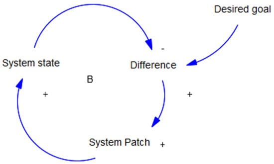
Figure 1.
Diagram causal of a balancing loop.
Figure 2 illustrates the typical behavior of a rolling model, where a production target for parts in the textile industry is established. The curve represents the system’s monitoring of this target, reflecting the ideal and desired behavior.
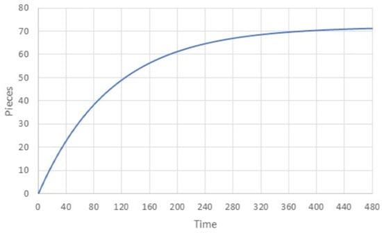
Figure 2.
Graph of the typical balancing loop in a textile application.
The main objective of this research project is to develop a mathematical model that allows a more detailed and precise understanding of the behavior of equilibrium loops in SD. These loops are vital to maintain stability and meet specific objectives within a simulation model.
The behavior of these balancing loops is usually based on ideal scenarios that do not fully reflect the complexity of reality. In practice, precise models can operate with varying efficiencies due to various irregularities and particularities. This discrepancy is the main engine of our research proposal, which seeks to offer a more realistic understanding of the behavior of the loops, considering their different levels of efficiency.
To achieve this objective, we propose the introduction of fractional calculation in SD models, with a specific focus on equilibrium loops. This innovative approach opens up new perspectives on the state of the art by offering a more accurate way to model and understand complex systems. By including fractional calculation, we can better capture the nonlinear nature and temporal dynamics of equilibrium loops, allowing us to effectively address efficiency variations and other irregularities in practice.
In this research, we focus on two departments of the textile process, which we represent as two balance loops. To obtain accurate and applicable data, we collaborate with a company in the southern state of Guanajuato. By analyzing these loops, we evaluate the efficiencies of the Overall Equipment Efficiency (OEE) model, providing valuable information for business managers’ decision-making. The final objective is to contribute to developing methodologies and tools that allow more effective and efficient management of complex systems in the industrial field and, in general, to the dynamics of systems.
Fractional calculus (FC) is a branch of mathematics based on the concept of derivatives and integrals of non-integer or fractional orders. This mathematical discipline has found a wide range of applications in various fields of knowledge from physics and biology to engineering and economics. One of the most prominent features of fractional calculus is its ability to model and understand complex phenomena that exhibit long-term dependencies and nonlinear behaviors.
In the realm of modeling physical systems, fractional calculus has been used to describe phenomena such as anomalous diffusion in porous media, particle dynamics in fractal media, and wave propagation in dispersive media. For example, in a study conducted by Podlubny [22], fractional calculus was applied to model contaminant diffusion in aquifers, allowing for a more accurate capture of contaminant propagation in complex hydrogeological systems.
Fractional calculus has proven helpful in understanding biological phenomena such as population dynamics, substance diffusion in biological tissues, and neuronal activity modeling. In a landmark paper by Mainardi [23], the applications of fractional calculus in modeling population dynamics were explored, highlighting its ability to capture the complexity of evolving biological systems.
In signal processing, fractional calculus has been used to model and analyze non-stationary signals and stochastic processes. For instance, in a study by Magin [24], fractional calculus was applied to develop nonlinear time series models, leading to a better understanding of temporal variability in experimental data.
Another innovative approach in fractional calculus is used to improve the accuracy of wind energy prediction [25], which is crucial for optimizing the operation of the electrical grid and harnessing renewable resources. Researchers propose a short-term memory model to forecast missing wind speed and direction data, and a fractional-order neural network (FONN) with a fractional activation function to enhance the prediction of generated wind energy. Through two case studies, the predictive effectiveness of the FONN model in wind power prediction is demonstrated. This hybrid approach improves forecast accuracy and addresses data gaps evaluated through mean errors and R2 values.
Another innovation involves presenting a new approach to numerically solving systems of fractional integro-differential equations [26]. Vieta–Fibonacci polynomials are used as essential functions, and the projection method for the fractional Caputo order is derived for the first time. This innovative approach involves an efficient transformation that reduces the problem to a system of two independent equations whose solution approximates the original problem. The efficiency and accuracy of the proposed method are validated, demonstrating the existence of a solution to the approximate problem and performing an error analysis. Numerical tests support theoretical interpretations.
Currently, FC is applied in a wide range of knowledge areas, including the analysis of viscoelastic models [27,28], fractional models of anomalous diffusion cf. [29], analysis of fractional-order electrical circuits as in [30], and medical image processing [31,32]. Additionally, the study of the role of vaccines in controlling the spread of COVID-19 involves fractional models of COVID-19 behavior when vaccines are applied [33]. These are just a few examples of applications.
Introducing fractional calculus into SD models represents a significant advancement with essential implications across various fields, including industrial engineering. This innovation enables a more precise description of complex systems, addressing nonlinear phenomena and long-term dependence. It results in a deeper understanding of constantly changing systems and more effective solutions in various disciplines.
In this study, we focused on using fractional calculus to describe the behavior of equilibrium loops in the presence of irregularities and particularities that hinder ideal behavior. However, it is essential to note that fractional models present an inherent limitation: they do not provide a precise definition of differential or geometry, which raises questions about their effectiveness. Several proposals have been made in recent years that attempt to give a physical and geometric interpretation to derivatives and integrals of non-integer order. Although there is no unified criterion, as in the case of integer operators, some phenomena, such as viscoelasticity, could not be explained in terms of whole operators. Moreover, violating the Leibniz rule allows fractional operators to be used in practical applications. In our work, fractional models seek to interpret the model’s efficiency (balancing loop) where the ideal case would correspond to an order of derivative equal to 1. Although there is no unified criterion regarding fractional calculus’s physical and geometric interpretation, some proposals have been made, such as [34,35,36]. On the other hand, Tarasov [37] proposes that one of the rules that fractional operators must meet is violating the Leibniz rule; this allows fractional calculation to be used in various physical applications.
Significant studies have focused on studying systems of integral-differential fractional equations in fractional calculus. These investigations stand out for their resolution through innovative numerical methods, simplifying the search for solutions [38,39]. However, the main strength of our research project lies in the fact that we offer an analytical solution to this type of equation, which represents a remarkable advance over previous approaches mainly focused on numerical strategies.
It is a versatile tool with multidisciplinary applications ranging from modeling physical and biological systems to process optimization. It has already been successfully applied in areas such as viscoelastic model analysis, anomalous diffusion, electrical circuits, and the study of COVID-19 propagation when vaccines are applied. This approach not only enriches the field of dynamic systems but also significantly impacts various areas of science and technology.
2. Materials and Methods
Fractional calculus (FC) is a discipline that studies fractional order integration and differentiation operators, meaning operators of non-integer order. Its origin dates back to the beginnings of conventional calculus when the first notations for derivatives were proposed [40]. Over the years, different definitions of fractional derivative have emerged, some based on the generalization of the limit definition of differentiation, such as the definition by Lacroix, the fractional derivative [41], and in recent years, the conformable derivative [42]. Others are based on the generalization of multiple integrations and the properties of semigroup, namely, the Riemann–Liouville fractional integral (IRL) and derivatives: Riemann–Liouville (DRL), Caputo derivative [43], Caputo–Fabrizio derivative (DCF) proposed in 2015 [44], and the Atangana–Baleanu derivative (AB) from 2016 [45].
2.1. Gamma Function
The factorial of an integer number is defined as the product of all consecutive integers from 1 to and is expressed:
where zero factorial is defined as 0! = 1. For an extension for values other than integers, use the Gamma function defined by the integral [46]:
for any ∈ , as to , when integrating by parts, you have an attractive property called recurrence property:
When applied to integer real values, we have the relation:
in this way, the factorial concept can be generalized for real or complex values.
2.2. Mittag-Leffler Function
Just as the exponential function plays a fundamental role in solving many ordinary differential equations, the Mittag-Leffler function (ML) [47], defined in 1903, consistently appears in the solution of fractional differential equations.
where , ∈ , α is an arbitrary parameter; subsequently, a generalization was proposed in 1905, and other updates in [48,49]. The function is
where α, ∈ are also arbitrary parameters, and the expression is called a two-parameter ML function.
where again, α, β, and γ C are arbitrary parameters, and the expression is called the Mittag-Leffler function of three parameters. When γ = 1, the equation becomes Equation (6). In addition, it can be observed that Equation (5) is a special case when β = 1 in the Equation (5). Therefore, the exponential function is considered a special case of ML when α = 1, that is:
The aforementioned is why the ML function and its generalizations are called generalized Mittag-Leffler functions. Research into the properties of the ML function has continued [50,51]. Let us consider the Laplace transforms of the following functions: Equations (9) and (10) in terms of the Mittag-Leffler function [52]:
where y , with .
2.3. Caputo Derivative
The fractional Caputo derivative was proposed in 1971 [43] to avoid the fractional order initial conditions of the Riemann–Liouville derivative. It is defined as follows: see Equation (11).
Definition 1.
Let
be a continuous function
where , y . And his Laplace transform is given by:
where , and . for n = 1 the Laplace transform is given by:
3. Methodology
In this investigation, the process begins with creating the system dynamics model, which is based on identifying and analyzing equilibrium loops and sets a specific goal to achieve. Then, we formulate the system of differential equations that govern the system’s behavior. Ordinary differential equations initially solve this system to obtain an initial solution. The OEE method is proposed, and the efficiencies of each department, which relate to alphas, are obtained. Later, fractional calculus is implemented using the Caputo method to solve fractional differential equations, allowing a more accurate description of the system’s behavior. Simulations are performed using these mathematical models for both the Tissue and Threading departments, providing a thorough evaluation of the system’s performance in different operating scenarios and conditions. This comprehensive methodological approach ensures a thorough and detailed understanding of the dynamics of the industrial processes studied, as shown in Figure 3.
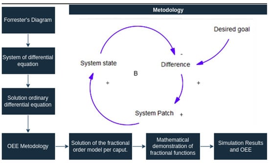
Figure 3.
System dynamics methodology introducing fractional calculation.
3.1. System Dynamics Model
The Forrester diagram, as shown in Figure 4, represents the dynamics of the textile production process through an SD model. This model shows the two fundamental departments of the textile process: Weaving and Basting. It comprises two state variables, x and y, representing these departments, respectively. These state variables are the system’s central axis, reflecting each department’s cumulative production. The diagram also incorporates six auxiliary variables and two flow variables, forming the system, interactions, and feedback mechanisms.
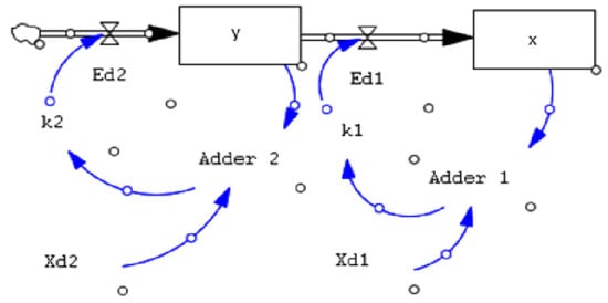
Figure 4.
System dynamics model in the Vensim environment.
The auxiliary variables, Xd1 and Xd2, are particularly prominent as they mean the system objectives or the target number of parts (for example, parts of a specific sweater model) that each department seeks to produce. These goals are not static; they guide operational dynamics, shaping workflow and production efforts within each department. The diagram also introduces adders 1 and 2, which calculate the discrepancy between the actual production and the targets set for each department, highlighting areas where adjustments may be needed to align with production targets.
The constant k, assigned to each department, represents the ideal rate at which the desired production level can be reached, expressed in units of (1/min). These constants are essential to calibrate the system to optimal performance, ensuring that production targets are met efficiently. Table 1 describes these variables’ specific values and roles in the Forrester diagram, providing a clear framework for understanding the dynamics at play.

Table 1.
Variables of the Forrester diagram.
3.2. System of Differential Equations
It is important to note that a system dynamics model has been developed to represent the production process in two departments. From this model, the two fundamental differential equations that describe the behavior of these departments, presented as Equations (14) and (15), have been identified and formulated. These equations form the analysis’s backbone, providing a detailed understanding of production dynamics in these specific contexts.
The proposed system, with initial conditions ,
3.3. Solution Ordinary Differential Equation
Equations (16) and (17) are obtained by solving the whole system of differential equations.
To obtain the values of , the solution of each of the state variables must be equal; it is equal to the operating time of each department, where they are 480 and 100 min, respectively; the value of k is sought, where 98% of the goal is obtained, obtaining a value of k1 = 0.009541 for the Weaving department and k2 = 0.12 for the Basting department.
3.4. OEE Methodology
The methodological approach of this study focuses on the Weaving and Basting departments, which are fundamental segments of the textile production chain. Working with a company located in the southern part of Guanajuato, real-world data were collected to assess these departments’ efficiency accurately. The evaluation leverages the Overall Equipment Effectiveness (OEE) methodology, a comprehensive measure that evaluates a department’s efficiency based on equipment availability, performance speed, and product quality. For this study, product quality is specifically related to the production of a particular model of sweater, underlining the practical application and relevance of this research for the operational challenges of the textile industry.
In this research project, fractional differential equations and their alpha value, which will be addressed, are intrinsically linked to the efficiency derived from the OEE methodology. Therefore, obtaining the absolute efficiency values of the company located south of Guanajuato is essential. These efficiency values are directly related to the fractional order of the derivative, underlining the importance of their accuracy and validity for proper modeling and understanding of the dynamics of the textile production process.
3.4.1. Availability Factor
Availability is calculated by dividing the actual operating time by the planned production time. This factor, expressed as a percentage, provides a key measure of operational efficiency by considering the time the equipment operates according to the established plan. The availability of the Weaving department for the week of October 25 to 30 can be observed in Table 2.
Table 2.
Availability of the Weaving department.
Table 3 shows the availability of the Basting department for the week of 25–30 October.
Table 3.
Availability of the Basting department.
3.4.2. Quality Factor
Quality in Overall Equipment Effectiveness (OEE) is measured by considering the units that meet quality standards against the total units produced. The quality factor of the Weaving department for the week of 25–30 October can be observed in Table 4.
Table 4.
Quality of the Weaving department.
Table 5 shows the quality factor of the Threading department of the week from 25–30 October.
Table 5.
Quality of the Basting department.
3.4.3. Performance Factor
Efficiency is measured by the planned production factor divided by the actual production. Table 6 shows the efficiency factor of the Basting department for the week of 25–30 October.
Table 6.
Performance of the Weaving department.
The performance factor of the Basting department for the week of 25–30 October can be observed in Table 7.
Table 7.
Performance of the Basting department.
The OEE factor is determined by multiplying the three key factors in the methodology. Table 8 details the efficiency calculation for the two departments.
Table 8.
Calculation of the OEE methodology in the departments.
Overall Equipment Effectiveness (OEE) was calculated for both departments, yielding an alpha value of 0.7790 for the tissue process and an alpha value of 0.9084 for the Threading department.
4. Results
In this work, the results obtained through the use of the derivative of Caputo are presented, accompanied by their demonstration and the corresponding graphic representations in function of time. These graphs show variations in system behavior under different levels of efficiency.
4.1. Solution of The Fractional Order Model Per Caputo
It is proposed to replace the first-order derivative operators of the system of differential equations with fractional-order operators of order α, where 0 < α < 1. When α = 1, it returns to the first-order operators and, therefore, to the original system of equations, see Equations (18) and (19).
When using the Caputo derivative operator in the system of fractional equations, we have:
To solve the system of fractional order differential equations, we apply the Laplace transform:
By simplifying both equations and applying the initial conditions, we obtain:
When resolving to :
we can find the solution by applying the inverse Laplace transform using the formula of Equation (10), so we have Equation (26).
To find the solution of , we can use of Equation (25):
Clearing for Y(s), we have:
To solve Y(s), we separate in two terms and , where the first has the same structure of X(s), therefore we can use the same formula of inverse transform and solve the first term:
applying Laplace transform to :
and for the second term we have:
where we multiply the denominator of by :
and by rearranging the denominator products, we obtain:
We apply the properties of the geometric series to both products: and :
Applying the properties of the series product we obtain a more compact format:
We express the argument of the series as a fraction and multiply it by :
and the products are rearranged in the denominator:
Now you can find the inverse transform:
and the solution of is given by:
4.2. Mathematical Demonstration of Fractional Functions
Demonstrating fractional functions is fundamental to validate the mathematical solidity and formality of the models developed. When considering the case where the alpha value equals 1, the fractional solution is expected to match the solution obtained by traditional methods. This coincidence demonstrates the consistency of the fractional approach with conventional methods and confirms the mathematical validity of the models. Therefore, the accuracy and coherence of the fractional approach in the representation of dynamic systems can be verified by comparing the solutions obtained with and without the use of fractional functions. This comparison is crucial to ensure that the mathematical tools are appropriate and effective in modeling complex phenomena.
The demonstration is performed for , starting from Equation (26) when :
Now, we replace it in the Mittag-Leffler function:
resulting in the denominator equal to =k!. Then, we have the Euler function:
replace the value of k, by Equation (16) is obtained by performing the demonstration.
Resulting in being equal to the ordinary solution by testing the correct solution by the Caputo method for state variable 1. The demonstration is performed for , when :
To demonstrate the function found with the fractional calculation when , we apply the Laplace transform, which divides the transformation into two parts:
The partial fractions solve the second term left in the equation as follows:
Later, the transform of the place is applied to the second part:
where the denominator passes to multiply the numerator in each of the summations.
The terms are arranged to obtain the geometric series in the two terms:
The approximation of the geometric series obtained is represented as follows:
The terms are arranged as follows:
Multiply and rearrange the denominator:
The linear partial fractions are made:
Resulting in the partial fractions:
multiplying and simplifying the equation.
are added
reducing similar terms and drawing common ground .
reducing similar terms in .
the common factor is removed in the equation.
Now, you can find the inverse transform in Equation (17):
Therefore, by checking that the solution obtained by the Caputo method of the fractional calculation, by substituting α = 1, which coincides with the function in ordinary time, we validate the fractional solution. This result confirms the consistency and precision of the fractional approach in the representation of dynamic systems. By evaluating both fractional functions in 1 and obtaining the function over time for the two state variables, the validity and reliability of the models developed are corroborated. This finding reinforces confidence in using fractional calculus as a practical mathematical tool to address complex dynamic phenomena.
4.3. Simulating Diverse Scenarios
In this section, we will explore several scenarios, varying both production goals and alpha values in each department, to better understand how these variables affect the performance of the Weaving and Basting process. This will provide valuable information for decision-making in the management of textile production.
4.3.1. Simulation of Weaving Department Efficiencies
It is important to note that the alpha parameter plays a fundamental role as an indicator of operational efficiency, and its range of variation allows a thorough assessment of the efficiency of the department in question. Table 9 shows the different scenarios for the Weaving department.
Table 9.
Parameter variance for different simulations of the Weaving department.
Figure 5 shows simulation 1, which compares the six efficiency categories with 100% performance.
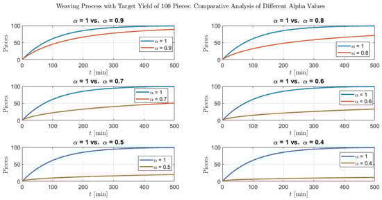
Figure 5.
Simulation 1 of the Weaving process.
Figure 6 shows simulation 2, which compares the six efficiency categories with 100% performance.
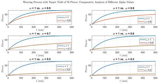
Figure 6.
Simulation 2 of the Weaving process.
Figure 7 shows simulation 3, which compares the six efficiency categories with 100% performance.
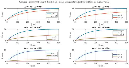
Figure 7.
Simulation 3 of the Weaving process.
4.3.2. Simulation of Basting Department Efficiencies
Table 10 details the different scenarios considered for the Basting department. Each scenario represents a unique combination of variables, including the department’s production goal and the efficiency values associated with the processes, expressed in alpha terms. These scenarios provide a comprehensive view of the possible configurations under which the performance of the Basting department in the manufacturing process is evaluated.
Table 10.
Parameter variance for different simulations of the Basting department.
Figure 8 shows simulation 1, which compares the six efficiency categories with 100% performance.
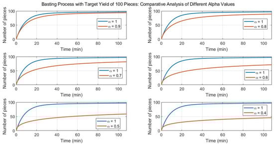
Figure 8.
Simulation 1 of the Basting process.
Figure 9 shows simulation 2, which compares the six efficiency categories with 100% performance.
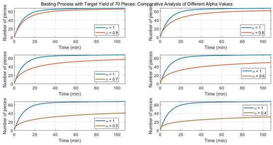
Figure 9.
Simulation 2 of the Basting process.
Figure 10 shows the third scenario for the Basting department, where the six comparative labels are shown.
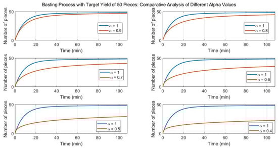
Figure 10.
Simulation 3 of the Basting process.
Simulations provide us with an invaluable tool for decision-making. By exploring a variety of scenarios that encompass different efficiency values for both departments, we can gain a deeper understanding of how these factors affect the production process. This ability to simulate and compare multiple scenarios gives us valuable insight to optimize our operations and make informed decisions that drive efficiency and productivity across the organization.
4.4. Field Validation
In this section, we contrast the efficiency of 100% with the efficiencies observed in each of the two departments validated in the field. This meticulous analysis allows us to see the operational reality of both departments. In addition, it allows us to identify significant discrepancies and areas of potential improvement, which contributes to more informed decision-making and continuous optimization of our processes.
4.4.1. Simulation of Weaving Department Efficiencies
The results of field validation using the OEE methodology are presented in Figure 11 and detailed in the third section. In this context, the efficiency obtained for the Weaving department was 77.90%.
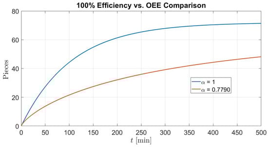
Figure 11.
Validation of Weaving department efficiencies.
4.4.2. Simulation of Basting Department Efficiencies
The results of field validation using the OEE methodology are presented in Figure 12 and detailed in the third section. In this context, the efficiency obtained for the Basting department was 90.84%. It can be concluded that the Weaving process is in the category “Good” since it exceeds 70% of estimated efficiency and has a wide margin for improvements in the two categories. It is estimated that it could achieve approximately 50 pieces. On the other hand, in the Basting process, it is in the “Optimum” category, exceeding 90% efficiency, which indicates a very good performance in this department, obtaining 67 pieces during the given period.
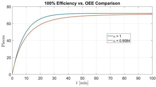
Figure 12.
Validation of Basting department efficiencies.
The results presented in Section 4.4 are specifically designed and analyzed for domain 0 < α < 1. This range was selected intentionally because it makes sense for the application. Since the value of α does not measure absolute production but production efficiency, it is limited to the range from 0 to 1. In this context, a value of α greater than 1 could indicate an efficiency greater than 100%, which would not be practical or relevant to interpreting efficiency in the process. Therefore, we focused on the range 0 < α < 1, where the results are most significant and applicable for this study.
5. Conclusions
This research project presents an innovative proposal by introducing fractional calculus into system dynamics models, explicitly focusing on equilibrium loops. By addressing discrepancies between ideal simulations and actual models, this initiative seeks to provide a more realistic understanding of systems’ behavior, considering their different levels of efficiency. The integration of fractional calculus significantly strengthens existing models, providing more accurate and helpful information for decision-making in various contexts. This contribution represents a valuable advance in the field of system dynamics in line with the legacy of engineer Jay Forrester.
The results obtained from the simulations in Figure 3 and Figure 4 reveal a series of significant findings. First, the validity of the solutions obtained by comparing ordinary differential equations with fractional solutions for different alpha values has been confirmed. This finding reinforces the solidity of the approach used in the study. In addition, the analysis of efficiency curves in the different areas of the company determines the completion time of orders based on the percentage OEE indicator. For example, in the Tissue department, with 91% efficiency. The proposed approach determines the respective duration time. This efficiency level highlights the importance of implementing continuous improvement strategies in production management to meet deliveries promptly. In short, the results provide a solid foundation for informed decision-making to diagnose company processes and improve overall performance. Future work will analyze the efficiency behavior of an industrial process using the theory of conformable calculus.
Author Contributions
Conceptualization, R.B.-S., J.M.B.-S. and L.M.-J.; Data Curation J.M.B.-S.; Formal Analysis J.M.B.-S., R.B.-S. and L.M.-J. Funding acquisition R.B.-S. and L.M.-J.; Methodology, J.M.B.-S. and R.B.-S.; Project Administration R.B.-S.; Resources R.B.-S.; Software J.M.B.-S., R.B.-S. and L.M.-J.; Supervision R.B.-S. Validation, J.M.B.-S., R.B.-S. and L.M.-J.; writing—original draft preparation, J.M.B.-S. writing—review and editing, J.M.B.-S., R.B.-S. and L.M.-J. All authors have read and agreed to the published version of the manuscript.
Funding
This research received no external funding.
Data Availability Statement
The algorithm developed in Matlab R2019a software that support the results of this study are available at the corresponding author on reasonable request.
Conflicts of Interest
The authors declare no conflicts of interest.
References
- García, J.M. Teoría y Ejercicios Prácticos de Dinámica de Sistemas: Dinámica de Sistemas con VENSIM PLE; Nova Science Publishers, Inc.: Hauppauge, NY, USA, 2023. [Google Scholar]
- Aracil, J.; Gordillo, F. Dinámica de Sistemas; Alianza Editorial: Madrid, Spain, 1997; p. 20. [Google Scholar]
- De Leo, E.; Aranda, D.; Addati, G. Introducción a la Dinámica de Sistemas; no. 739, Serie Documentos de Trabajo; University of CEMA: Buenos Aires, Argentina, 2020. [Google Scholar]
- Spinel, A.V. Análisis de Armónicos en Redes de Distribución con Recursos Renovables Conectados a Través de Inversores; Universidad De Los Andes: Bogota, Colombia, 2023. [Google Scholar]
- Abid, A.; Kallel, I.; Sanchez-Medina, J.; Ayed, M. Parameters Sensitivity Analysis of Ant Colony Based Clustering: Application for Student Grouping in Collaborative Learning Environment. IEEE Access 2023, 12, 24751–24761. [Google Scholar] [CrossRef]
- Cazcarro, I.; García-Gusano, D.; Iribarren, D.; Linares, P.; Romero, J.; Arocena, P.; Arto, I.; Banacloche, S.; Lechón, Y.; Miguel, L.; et al. Energy-socio-economic-environmental modelling for the EU energy and post-COVID-19 transitions. Sci. Total Environ. 2022, 805, 150329. [Google Scholar] [CrossRef] [PubMed]
- Angerhofer, B.; Angelides, M. System dynamics modelling in supply chain management: Research review. In Proceedings of the 2000 Winter Simulation Conference Proceedings (Cat. No.00CH37165), Orlando, FL, USA, 10–13 December 2000. [Google Scholar]
- Zimmermann, N.; Curran, K. Dynamics of interdisciplinarity: A microlevel analysis of communication and facilitation in a group model—Building workshop. Syst. Dyn. Rev. 2023, 39, 336–370. [Google Scholar] [CrossRef]
- Ortega, J.J.C.; Serrato, R.B.; Morales, R.A.L. Development of a system dynamics model based on Six Sigma methodology. Ing. Investig. 2017, 37, 80. [Google Scholar] [CrossRef][Green Version]
- Wang, Z.; Li, X.; Mao, Y.; Li, L.; Wang, X.; Lin, Q. Dynamic simulation of land use change and assessment of carbon storage based on climate change scenarios at the city level: A case study of Bortala, China. Ecol. Indic. 2022, 134, 108499. [Google Scholar] [CrossRef]
- Zoghi, M.; Kim, S. Dynamic Modeling for Life Cycle Cost Analysis of BIM-Based Construction Waste Management. Sustainability 2020, 12, 2483. [Google Scholar] [CrossRef]
- Liu, J.; Liu, Y.; Wang, X. An environmental assessment model of construction and demolition waste based on system dynamics: A case study in Guangzhou. Environ. Sci. Pollut. Res. 2020, 27, 37237–37259. [Google Scholar] [CrossRef]
- De-Blas, I.; Miguel, L.; De-Castro, C. Modelos de evaluación integrada (IAMs) aplicados al cambio climático y la transición energética. DYNA-Ing. Ind. 2021, 96, 316. [Google Scholar]
- Sánchez, J.B.; Serrato, R.B.; Bianchetti, M. Design and Development of a Mathematical Model for an Industrial Process, in a System Dynamics Environment. Appl. Sci. 2022, 12, 9855. [Google Scholar] [CrossRef]
- Mojtahedzadeh, M.; Qureshi, H.I. Understanding End of Life Practices: Perspectives on Communication, Religion and Culture; Springer International Publishing: Berlin/Heidelberg, Germany, 1997; pp. 261–274. [Google Scholar]
- Mojtahedzadeh, M. Do parallel lines meet? How can pathway participation metrics and eigenvalue analysis produce similar results? Syst. Dyn. Rev. 2008, 24, 451–478. [Google Scholar] [CrossRef]
- Gonçalves, P. Behavior Modes, Pathways and Overall Trajectories: Eigenvector and Eigenvalue Analysis of Dynamic Systems. SSRN Electron. J. 2009, 25, 35–62. [Google Scholar] [CrossRef]
- Oliva, R. Structural dominance analysis of large and stochastic models. Syst. Dyn. Rev. 2016, 32, 26–51. [Google Scholar] [CrossRef]
- Schoenberg, W.; Hayward, J.; Eberlein, R. Improving Loops that Matter. Syst. Dyn. Rev. 2023, 39, 140–151. [Google Scholar] [CrossRef]
- Sánchez, J.M.B.; Serrato, R.B. Design and Development of an Optimal Control Model in System Dynamics through State-Space Representation. Appl. Sci. 2023, 13, 7154. [Google Scholar] [CrossRef]
- Sterman, J. Business Dynamics; Irwin/McGraw-Hill: New York, NY, USA, 2010; p. 982. [Google Scholar]
- Podlubny, I. Fractional Differential Equations: An Introduction to Fractional Derivatives, Fractional Differential Equations, to Methods of Their Solution and Some of Their Applications; Elsevier: Amsterdam, The Netherlands, 1998. [Google Scholar]
- Mainardi, F. Fractional Calculus: Some Basic Problems in Continuum and Statistical Mechanics; Springer: Vienna, Austria, 1997; pp. 291–348. [Google Scholar]
- Magin, R. Fractional Calculus in Bioengineering, Part 1. Critical Reviews™. Biomed. Eng. 2004, 32, 104. [Google Scholar]
- Ramadevi, B.; Kasi, V.R.; Bingi, K. Hybrid LSTM-Based Fractional-Order Neural Network for Jeju Island’s Wind Farm Power Forecasting. Fractal Fract. 2024, 8, 149. [Google Scholar] [CrossRef]
- Moumen, A.; Mennouni, A.; Bouye, M. A Novel Vieta–Fibonacci Projection Method for Solving a System of Fractional In-tegrodifferential Equations. Mathematics 2023, 11, 3985. [Google Scholar] [CrossRef]
- Schiessel, H.; Metzler, R.; Blumen, A.; Nonnenmacher, T.F. Generalized viscoelastic models: Their fractional equations with solutions. J. Phys. A Math. Gen. 1995, 28, 6567–6584. [Google Scholar] [CrossRef]
- Meral, F.C.; Royston, T.J.; Magin, R. Fractional calculus in viscoelasticity: An experimental study. Commun. Nonlinear Sci. Numer. Simul. 2010, 15, 939–945. [Google Scholar] [CrossRef]
- Chen, W.; Sun, H.; Zhang, X.; Korošak, D. Anomalous diffusion modeling by fractal and fractional derivatives. Comput. Math. Appl. 2010, 59, 1754–1758. [Google Scholar] [CrossRef]
- Guia, M.; Gomez, F.; Rosales, J. Lomé and the North-South Relations (1975–1984): From the “New International Economic Order” to a New Conditionality. In Europe in a Globalising World; Nomos: Baden-Baden, Germany, 2013; Volume 11, pp. 123–146. [Google Scholar]
- Leonardo, M.-J.; Pedro, L.-L.; Adán, F.-B.; Manuel, L.-H.J. Automatic blood vessel detection using fractional Hessian matrices. ECORFAN J. 2022, 6, 12–19. [Google Scholar]
- Sengupta, S.; Ghosh, U.; Sarkar, S.; Das, S. Prediction of Ventricular Hypertrophy of Heart Using Fractional Calculus. J. Appl. Nonlinear Dyn. 2020, 9, 287–305. [Google Scholar] [CrossRef]
- Baba, I.A.; Humphries, U.W.; Rihan, F.A. Role of Vaccines in Controlling the Spread of COVID-19: A Fractional-Order Model. Vaccines 2023, 11, 145. [Google Scholar] [CrossRef] [PubMed]
- Ruby; Mandal, M. The geometrical and physical interpretation of fractional order derivatives for a general class of functions. Math. Methods Appl. Sci. 2024, 2024, 1–21. [Google Scholar] [CrossRef]
- Podlubny, I. Geometric and Physical Interpretation of Fractional Integration and Fractional Differentiation. arXiv 2001, arXiv:math/0110241. [Google Scholar]
- Heymans, N.; Podlubny, I. Physical interpretation of initial conditions for fractional differential equations with Riemann-Liouville fractional derivatives. Rheol. Acta 2006, 45, 765–771. [Google Scholar] [CrossRef]
- Tarasov, V.E. No violation of the Leibniz rule. No fractional derivative. Commun. Nonlinear Sci. Numer. Simul. 2013, 18, 2945–2948. [Google Scholar] [CrossRef]
- Micula, S. An iterative numerical method for fractional integral equations of the second kind. J. Comput. Appl. Math. 2018, 339, 124–133. [Google Scholar] [CrossRef]
- Jafari, H.; Tuan, N.; Ganji, R. A new numerical scheme for solving pantograph type nonlinear fractional integro-differential equations. J. King Saud Univ.—Sci. 2021, 33, 101185. [Google Scholar] [CrossRef]
- Sánchez-Muñoz, J. Hamilton y el descubrimiento de los Cuaterniones. Pensam. Matemático 2011, 7. [Google Scholar]
- De Oliveira, E.C.; Machado, T. A review of definitions for fractional derivatives and integral. Math. Probl. Eng. 2014, 2014, 1–6. [Google Scholar] [CrossRef]
- Khalil, R.; Al Horani, M.; Yousef, A.; Sababheh, M. A new definition of fractional derivative. J. Comput. Appl. Math. 2014, 264, 65–70. [Google Scholar] [CrossRef]
- Caputo, M.; Mainardi, F. A new dissipation model based on memory mechanism. Pure Appl. Geophys. 1971, 91, 134–147. [Google Scholar] [CrossRef]
- Caputo, M.; Fabrizio, M. Theory and Applications of Fractional Order Systems. Progr. Fract. Differ. Appl. 2015, 1, 73–85. [Google Scholar]
- Atangana, A.; Baleanu, D. New fractional derivatives with nonlocal and non-singular kernel: Theory and application to heat transfer model. Therm. Sci. 2016, 20, 763–769. [Google Scholar] [CrossRef]
- Artin, E. The Gamma Function; Courier Dover Publications: Mineola, NY, USA, 2015. [Google Scholar]
- Mittag-Leffler, G. Sur la représentation analytique d’une branche uniforme d’une fonction monogène: Seconde note. Acta Math. 1903, 24, 183–204. [Google Scholar] [CrossRef]
- Wiman, A. Über die Nullstellen der Funktionen E a (x). Acta Math. 1905, 29, 217–234. [Google Scholar] [CrossRef]
- Wiman, A. Über den Fundamentalsatz in der Teorie der Funktionen E a (x). Acta Math. 1905, 29, 191–201. [Google Scholar] [CrossRef]
- Zarslan, M.A.; Yılmaz, B. The extended Mittag-Leffler function and its properties. J. Inequalities Appl. 2014, 2014, 1–10. [Google Scholar] [CrossRef]
- Khan, M.A.; Ahmed, S. On some properties of the generalized Mittag-Leffler function. SpringerPlus 2013, 2, 337. [Google Scholar] [CrossRef]
- Makris, N. The Fractional Derivative of the Dirac Delta Function and Additional Results on the Inverse Laplace Transform of Irrational Functions. Fractal Fract. 2021, 5, 18. [Google Scholar] [CrossRef]


Disclaimer/Publisher’s Note: The statements, opinions and data contained in all publications are solely those of the individual author(s) and contributor(s) and not of MDPI and/or the editor(s). MDPI and/or the editor(s) disclaim responsibility for any injury to people or property resulting from any ideas, methods, instructions or products referred to in the content. |
© 2024 by the authors. Licensee MDPI, Basel, Switzerland. This article is an open access article distributed under the terms and conditions of the Creative Commons Attribution (CC BY) license (https://creativecommons.org/licenses/by/4.0/).