Abstract
This work introduces an alternative approach for developing a customized Metaheuristic (MH) tailored for tuning a Fractional-Order Proportional-Integral-Derivative (FOPID) controller within an Automatic Voltage Regulator (AVR) system. Leveraging an Automated Algorithm Design (AAD) methodology, our strategy generates MHs by utilizing a population-based Search Operator (SO) domain, thus minimizing human-induced bias. This approach eliminates the need for manual coding or the daunting task of selecting an optimal algorithm from a vast collection of the current literature. The devised MH consists of two distinct SOs: a dynamic swarm perturbator succeeded by a Metropolis-type selector and a genetic crossover perturbator, followed by another Metropolis-type selector. This MH fine-tunes the FOPID controller’s parameters, aiming to enhance control performance by reducing overshoot, rise time, and settling time. Our research includes a comparative analysis with similar studies, revealing that our tailored MH significantly improves the FOPID controller’s speed by 1.69 times while virtually eliminating overshoot. Plus, we assess the tuned FOPID controller’s resilience against internal disturbances within AVR subsystems. The study also explores two facets of control performance: the impact of fractional orders on conventional PID controller efficiency and the delineating of a confidence region for stable and satisfactory AVR operation. This work’s main contributions are introducing an innovative method for deriving efficient MHs in electrical engineering and control systems and demonstrating the substantial benefits of precise controller tuning, as evidenced by the superior performance of our customized MH compared to existing solutions.
1. Introduction
Today’s demand for a high-quality power supply presents a significant challenge as consumers require a stable and reliable source. Specifically, maintaining two critical parameters, frequency and voltage, at their established reference values is essential for system stability and reliability [1,2]. The frequency changes in electrical systems are linked to the dynamics of active power flow, whereas voltage fluctuations are closely associated with reactive power flow [3]. This highlights the importance of the relationship between power quality and stability, emphasizing the need for devices that can effectively compensate for these fluctuations in current electrical systems. Several devices are designed to address this issue, such as the bank of capacitors [4], synchronous compensators [5], Static Voltage Compensators (SVCs) [6], and Automatic Voltage Regulators (AVRs) [7,8], each playing a vital role in enhancing system performance and stability.
This work studies the AVR system as a device that regulates voltage variations, providing a constant power supply. Thus, AVR stands out for ensuring that the power of the generators and voltage supplied to end users are maintained within the specified margins despite the fluctuations in the electrical grid. Its principal function is to control the excitation of synchronous generators, the chief power production units of the entire power system. This process adjusts the excitation current and changes in the reactive power, fast controlling the voltage at the terminals. Still, the AVR system presents features that can harm the electrical system, such as oscillations, high overshoot, and errors in the steady state [8]. So, including reliable control in the system is essential to solving these problems. Although there is a wide range of modern controllers, the traditional Proportional-Integral-Derivative (PID) controller is the most widely used in industrial processes due to its versatility and straightforward implementation [9,10]. Nonetheless, implementing a classical PID controller could limit the transient performance in real systems. For this reason, an improved variant that provides a transient response with better features just appeared in the literature as a fractional-order PID controller (FOPID) [11,12,13]. However, an additional problem stems: fine-tuning an FOPID controller is more challenging than a traditional PID controller. In an FOPID, two additional adjusting parameters are added to the PID controller, corresponding to the fractional orders of the integral () and derivative () actions. These parameters can provide greater flexibility and ensure greater robustness [14]. Several traditional methods, such as “trial and error” and the Ziegler-Nichols (ZN), have been adopted to tune the FOPID controllers [10,15]. On the one hand, the “trial and error” method demands extensive designer experience, without mentioning that it is also a time-consuming process that does not guarantee the proper controller gains. On the other hand, ZN-based tuning requires exhaustive controller fine-tuning to obtain the desired response [8,16]. As an alternative to these traditional strategies, modern optimization methods like Metaheuristics (MHs) are implemented to efficiently search within a feasible solution space for the best controller gains.
MHs, recognized for their effectiveness and widespread adoption, have been essential in improving FOPID control performance in AVR systems [15]. Some examples include using MHs such as Simulated Annealing, Cuckoo Search [17], Particle Swarm Optimization [18], and Improved Marine Predators Algorithm [19] to optimize relevant control features such as overshoot, steady-state error, peak, rise, and settling times. Similarly, other authors have opted to improve these features by adding the Integral Time Absolute Error (ITAE) to the fitness functions [7].
Despite considerable progress in this field, the No-Free-Lunch theorem is highly relevant in optimization design. It implies that no MH, including those mentioned above, is guaranteed to be the most suitable for this kind of application without deeper analysis. Furthermore, the literature proliferates on analyzing this kind of solvers, some with a solid mathematical formulation [20,21,22], but others considered as “novel” are based on nature metaphors, leaving aside originality and losing sight of mathematical formalism. In fact, most “novel” MHs are variations of already classical MHs [23,24,25]. Therefore, a systematic and objective methodology is needed to tailor MHs for specific problems.
In response, the Automated Algorithm Design (AAD) approach offers promising solution alternatives [26]. One of its main advantages is that it avoids the user having to adapt algorithms to each problem manually. This manual process can be tedious and requires considerable time to build and verify the algorithms. Several studies based on AAD have proposed to obtain MHs [27,28]. The automated design of MHs is a relatively new paradigm, along with the automated algorithm configuration and selection [29]. The approach comes with obtaining a customized MH from an optimization problem or a family of problems. It consists of finding the combination of Search Operators (SOs) from the design space that deliver the best performance when applied to the optimization process. The best composition of custom MHs can be approached using Hyper-Heuristics (HH) [30]. In this context, an HH is a search strategy with or without learning capabilities for selecting or generating heuristic-based algorithms to solve computational search problems [31]. Hence, solving this problem requires defining a search space, employing some optimization algorithm to explore, and finding the operators that deliver the best performance for the customized MH.
Our research addresses two approaches. The former encompasses an AAD methodology for the automatic generation of a customized MH to optimize FOPID controllers for AVR systems. The latter consists of an in-depth influence analysis of the fractional orders over control features such as settling time and overshoot. To do so, this work uses CUSTOMHyS as a reliable and effective framework for obtaining custom MHs automatically. The reason is the proven success in practical engineering applications [32]. Furthermore, our study provides two landscapes for explaining in detail the dynamics of FOPID controllers. We also conduct a comparative study against works conceived under similar operational conditions, i.e., FOPID controllers designed through MHs for AVR systems. The results demonstrated the feasibility of this high-level strategy, providing high repeatability and performance to obtain an MH automatically to solve low-level problems (e.g., FOPID controller tuning). Using AAD-based methodologies, users can leverage automatic customizing and selecting MHs, thus focusing only on posing the low-level problem and fine-tuning the MH.
The main contributions of this work are described below:
- 1.
- This study demonstrates the advantages, reliability, and high performance of automatically designed tuners (i.e., MHs) for FOPID controllers in AVR systems.
- 2.
- It identifies and validates the optimal gain settings of the FOPID controller, ensuring it effectively compensates for the AVR system’s dynamics.
- 3.
- This work develops performance tests of the proposed FOPID controller, utilizing benchmark analysis that incorporates system disturbances, providing a comprehensive evaluation of its effectiveness.
- 4.
- Lastly, it presents a landscape analysis, focusing on the overshoot and settling time characteristics as the controller’s fractional components are varied. This analysis confirms the controller’s optimal configuration, enhancing system stability and performance.
The remainder of this document is organized as follows: Section 2 describes the key concepts that support this research. Then, Section 3 delves into the experiments’ methodology. Section 4 discusses the experiments’ outcomes. Finally, Section 5 summarizes the most relevant contributions and highlights future research directions of this work.
2. Foundations
This section overviews the Automatic Voltage Regulator system, followed by an introduction to fractional calculus, fractional-order PID controllers, metaheuristic optimization, and the automated algorithm design paradigm.
2.1. Automatic Voltage Regulator System
The Automatic Voltage Regulator (AVR) system is a vital technology solution for electrical systems’ generation and distribution stages [33]. It is an electrical device that automatically adjusts the voltage of one or more phases from the grid in response to changes in input voltage, load fluctuations, and other external factors. The main objective is maintaining a synchronous generator’s terminal voltage at a reference level. This regulation avoids damaging voltage fluctuations in connected devices that can reduce their lifetime and efficiency.
A basic AVR system consists of four components: amplifier, exciter, generator, and sensor, as shown in Figure 1a.
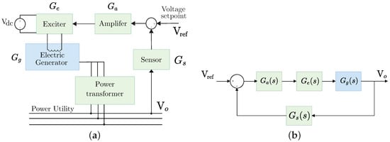
Figure 1.
Automatic Voltage Regulation (AVR) system: (a) Schematic of the AVR components, showing the exciter (), amplifier (), sensor (), electric generator (), and power transformer. (b) Uncontrolled model displaying the transfer functions for the exciter , amplifier , and sensor in relation to the output voltage .
In the first stage, the sensing block () is critical in the regulator operation since it establishes the basis for all subsequent corrective actions. Its primary purpose is accurately measuring the present voltage at the load or the power system’s output. Next, it is necessary to quantify the signal error (e [V]), i.e., the difference between the actual voltage ( [V]) and the desired voltage ( [V]) is measured as follows,
This stage determines the voltage level to be adjusted and is, in practice, the input to the control stages. Following Figure 1a, the amplifier () serves to amplify the error signal to regulate the power of the exciter (). This last component receives the amplified signal and acts on the generator to modify the magnetic field in a coil, adjusting the generated voltage in response. Notably, the generator () converts the mechanical energy into electrical energy.
The model shown in Figure 1b provided the transfer function to describe mathematically the AVR system. However, a linearization process must be performed to obtain the mathematical model of each component of the AVR system, considering the relevant time constants, ignoring saturation and nonlinearities [34]. The parameter values used in this work were selected based on [8,34] to define the transfer functions of each stage in the AVR system, as shown in Table 1. Lastly, the total transfer function of the AVR system is defined as

Table 1.
Subsystems and their transfer functions of the Automatic Voltage Regulation (AVR) implemented in this work.
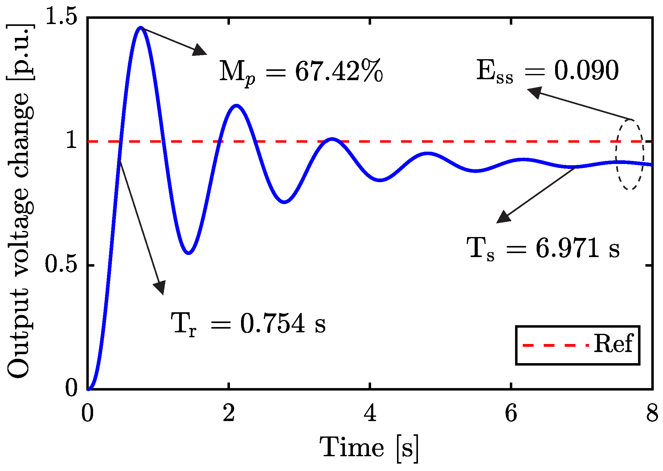
Figure 2 shows the uncontrolled transient response of the AVR system.
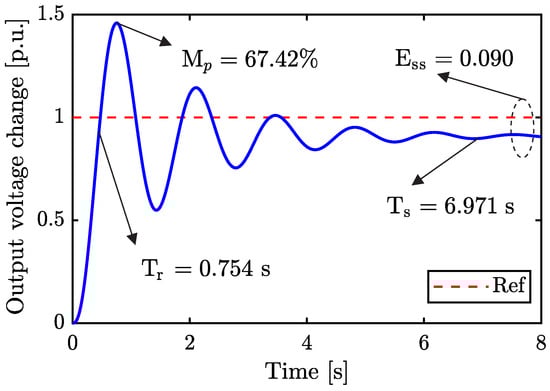
Figure 2.
Uncontrolled output voltage of the AVR system. It also details the overshoot ( [%]), settling time ( [s]), rise time ( [s]), and steady-state error ( [p.u.]).
It is noteworthy that such a response presents undesired behaviors, including a high overshoot ( = 67.42%), settling time ( = 6.971 s) and rise time ( = 0.754 s), as well as a considerable steady-state error ( = 0.090 p.u.). Thus, selecting a suitable controller may guide the system dynamics to improve the electrical output features.
2.2. Fractional Calculus
Fractional Calculus provides the theory to generalize the classical integro-differential operator utility through a non-integer order integro-differential operator denoted by [35,36]. In this context, the symbol corresponds to the fractional order that serves to define fractional integrals and derivatives into a single expression as follows,
since represents the operation’s order and can be any arbitrary real number in practical applications, where is the initial operating point and t is the working variable. Without loss of generality, we assume that t is dimensionless.
Several definitions of fractional integration and differentiation exist, each with its particular suitability for engineering modeling. Notably, the Grünwald-Letnikov (G-L) [37], Riemann-Liouville (R-L) [38], and Caputo’s [39] definitions stand out for their relevance and application in this field. A paramount work that provides a comprehensive framework for understanding fractional signal processing, leveraging the Liouville approach to explore various coherent formulations from suitable derivative definitions, can be read at [40].
The G-L fractional operator is often used in simulations because it can be directly applied to the numerical evaluation of fractional order derivatives [41]. This operator is given by
where is the Gamma function and since [35]. By its side, the R-L definition for the -order fractional derivative of a function is given as follows [38],
where and . Another important fractional derivative definition is Caputo’s formula, which is a particular case of the R-L formula to incorporate initial conditions in solving boundary value problems [40]. In the Caputo’s sense, the -order derivative of a function is described as,
since and .
Furthermore, the Laplace transform is beneficial when considering Zero Initial Condition (ZIC) and a causal system, i.e., . Recall the Laplace transform of f, , given by
where is the complex variable, with real numbers and . The Laplace transform corresponding to the nth ordinary derivative, regarding the continuity conditions on [38], corresponds to
Therefore, the Laplace transforms of the fractional order derivatives described above, according to [35], are
These transforms provide insight into the behavior of fractional-order systems and offer a pathway to the analytical and numerical methods required for solving complex problems in engineering and physics.
2.3. Fractional-Order Proportional-Integral-Derivative Controller
Traditional control structures, such as Proportional-Integral-Derivative (PID) controllers and their variants, are widely used in engineering applications due to their straightforwardness, efficacy, and constant improvement in tuning methodologies [42]. Mathematically, a PID control action is defined as,
where is the error between the set-point and output voltage , as well as , , and are the proportional, integral, and derivative gains. In addition, the corresponding transfer function using the Laplace transform is determined as follows,
Nonetheless, these conventional structures may fall short in some operational conditions, e.g., reduced overshoot and rapid settling times. In this context, fractional calculus is a promising alternative to enhance the performance of such conventional approaches by introducing fractional orders in the integral and derivative components to achieve more robust control responses.
The Fractional-Order Proportional-Integral-Derivative (FOPID) controller is a generalized version of the traditional PID controller, including two additional fractional order parameters, which Podlubny first introduced in [35]. These two parameters add various damping properties to the controller response over a more comprehensive frequency range, allowing for better results in higher-order, non-linear, and non-minimum-phase systems [43]. Another significant advantage of these controllers is their ability to decrease overshoot in the system response using the fractional derivative parameter, as discussed by Tejado et al. [44]. Finally, these controllers also improve other operational features such as rise time and settling time [45].
The FOPID control action is formally described in the time domain as
since and are the fractional orders designated to the integral and derivative components. In the frequency domain, assuming ZICs, the transfer function of the FOPID control in the Laplace domain can be expressed as
where support the FOPID structure. Adding fractional variables to the PID controller increases the design complexity. However, this action leads to significant flexibility since it permits a wider variety of tuning parameters and system responses, enhancing the response to disturbances [46].
2.4. Metaheuristics
Metaheuristics (MHs) are algorithmic strategies recognized by their flexibility and excellent performance in solving optimization problems [47]. They also incorporate mechanisms to circumvent premature convergence and detect satisfactory solutions within the search space [48]. In general, MHs are inspired by various phenomena observed in nature, a feature that often associates them with metaphors. Although these metaphors are fine in some MHs because they reveal clear ideas about their actual computational process [49], others are mere delusional stories. In this sense, we prefer to study MHs as linked functional blocks [50]. Thus, an MH can be described using three components: an initializer , one or more Search Operators (SOs) , and an finalizer . All these correspond to simple heuristics that interact directly or indirectly with the problem’s search space to solve [51]. So, an MH can be constructed using the following definitions.
Definition 1
(Metaheuristic). Consider MH as an iterative method that finds an optimal solution, denoted as , for the optimization problem at hand, which is guided by the fitness function . So, a finite sequence of operators defines the algorithm applied iteratively until fulfilling the stopping criterion, as detailed below:
where ∘ is the composition operator. Besides is an initializer, is the search operator, and is a finalizer. These simple heuristics are described in the following remarks.
Remark 1
(Initializer). Consider : as an operator that creates a candidate solution within the search space from scratch, where , and is the arbitrary domain. Since this work focuses on a continuous optimization problem, the domain corresponds to .
Remark 2
(Search Operator). Consider : as the search operator that alters a candidate solution , such that . To do so, the search operator encompasses two operations: perturbation () and selection (), i.e., . Note that the always perturbator precedes the selector. Besides, a search operator can be composed of two or more search operators, such as [50].
Remark 3
(Perturbators and Selectors). Consider as simple heuristics that transform and update , thus affecting the current solution . So, draws a perturbated version of a given candidate solution , and decides if this version will replace the original candidate solution .
Remark 4
(Finalizer). Consider as an operator that evaluates the quality of the current solution to determine the appropriate search operator to utilize. This operator uses the information of the solution state, i.e., fitness value, current iteration, and previous candidate solutions, among other features, considering a criteria function : .
For example, according to the previous definitions, a metaheuristic can be explicitly rewritten for an algorithm with two SOs via (16), as shown
which can describe many classical MHs, such as the well-known Genetic Algorithm (GA) that consists of two search operators, i.e., two perturbators and two selectors [52,53]. The first SO comprises a perturbator belonging to the Genetic Crossover () family followed by a Direct Selector (). The second SO is a perturbator belonging to the Genetic Mutation () family, followed by a Greedy Selector ().
Table 2 summarizes the SOs used in this work. It is a collection that considers different variation parameters and hyper-parameters, which in our implementation were predefined values, rendering 205 ready-to-use SOs. In addition, each operator has four selector versions, except for Random Search, which only uses a greedy type selector. For further details, please see [30].
Table 2.
Search operators that comprise the heuristic space with their variants of perturbators, selectors, and hyper-parameters.
2.5. Automated Algorithm Design
Automated Algorithm Design (AAD) has gained significant importance recently. Several AAD proposals can be found in the literature, but they always seek to avoid the bias caused by the algorithm designer. Although there are experts who can adjust or design algorithms appropriately, these processes are usually carried out through trial-and-error testing [54]. In this context, it is frequent that an algorithm does not offer the best performance because the multiple available alternatives were not explored when designing. However, proposals such as the Iterated Racing for Automatic Algorithm Configuration (irace) method [55] focus on the optimal selection and adjustment of the algorithm’s hyper-parameters. This approach is based on competitions or “races” in which different configurations of hyper-parameters are evaluated on a set of problem instances.
Another approach involves modularly building algorithms to select the best sequence of elements to solve a particular problem. Recently, Cruz-Duarte et al. [53] developed the CUSTOMHyS framework, which provided a structured strategy to obtain MHs by combining simple heuristics extracted from well-known MHs. Thus, the two design strategies described above fit the model-free and model-based strategies, respectively [56].
This work uses the model-based category to obtain MHs to solve continuous optimization problems by addressing the Metaheuristic Combinatorial Optimization Problem (MCOP) [50]. In this case study, the CUSTOMHyS framework generates a tailored MH to tune the FOPID controller for an AVR system. In addition, an Hyper-Heuristic (HH) is employed as a high-level solver for the MCOP, helping to explore the design space to identify efficient configurations. So, an HH can be any algorithm that can achieve a tailored MH by dealing with the following problem,
Hence, the fundamental task of an HH is to solve an optimization problem but at a high level. It must search within a heuristic space a feasible sequence of search operators (composing a selection heuristic with a perturbator heuristic, i.e., ) to achieve the metaheuristic () with the best performance or quality for a given problem (family) [50]. In this context, represents the number of SOs blending the MH.
Moreover, is a solver with a low abstraction level, i.e., it interacts directly with the particular problem , where is the search space, D is the problem dimensionality, and f is an objective function of the optimization problem. Readers are referred to [30,57] for a more in-depth review of HH concepts.
3. Methodology
This research was divided into three stages. The first was devoted to the HH process to obtain the customized MH. For this purpose, a collection of 205 SOs was employed as the heuristic space, combining the perturbators and selectors listed in Table 2 with variation parameters and hyper-parameters predefined. We utilized Simulated Annealing (SA) as the hyper-heuristic, namely SAHH, to control the search actions within the heuristic space. So SAHH employed a set of ten simple heuristics to guide the search process; some include add, remove, shift, swap, restart, mirror, and roll actions. Plus, SAHH hyper-parameters include an initial dimensionless temperature, a minimum dimensionless temperature, and a cooling rate set to 1.0, , and , respectively. These values were selected from several preliminary studies and statistical tests reported in [30]. For the HH process, a population size of 20 with a maximum number of 30 iterations for each candidate MH was set. In addition, 10 HH steps were defined, and each candidate’s MH was run 20 times to obtain the respective performance metric defined by
since med is the median, and iqr is the interquartile range of the last fitness values achieved during the runs . So, this metric checks the HH process improvement level. The idea is to select the array of SOs, i.e., the tailored MH, that best adapts to the optimization low-level problem and achieves fast convergence and repeatability of the obtained data. It is critical to clarify that the current process aims to create a customized metaheuristic (MH) specifically tailored to a given problem. Therefore, the outcome of the first stage is the MH itself rather than the solution to the low-level problem related to the controller tuning. At this stage, the low-level optimization problem has not been explicitly addressed. Once the MH is tailored to the problem family, it can be implemented similarly to other metaheuristics without repeating the HH process.
Algorithm 1 summarizes the SAHH implemented for solving the MCOP in (18). The process starts by randomly selecting a search operator from the heuristic space to generate a candidate solution from scratch. This initial sequence of SOs is used to assemble an MH according to Definition 1. Subsequently, the current MH is executed times, recording all the obtained fitness values and other measurements to evaluate its performance. Such a performance is assessed via (19). Next, SAHH generates a neighbor of the current heuristic sequence by picking up an action such as add, remove, or shift random heuristics. When add or shift actions are selected, simple heuristics are sampled from the collection of search operators. Subsequently, the MH is updated with these heuristics and evaluated as before. The internal steps of Algorithm 1 correspond to the procedure commonly found in SA implementations.
Operatively, each candidate MH is subjected to the low-level problem, which aims to tune the FOPID controller, represented in a five-dimensional domain; i.e., , with , , , and . Besides, the objective function associated with this problem is given by
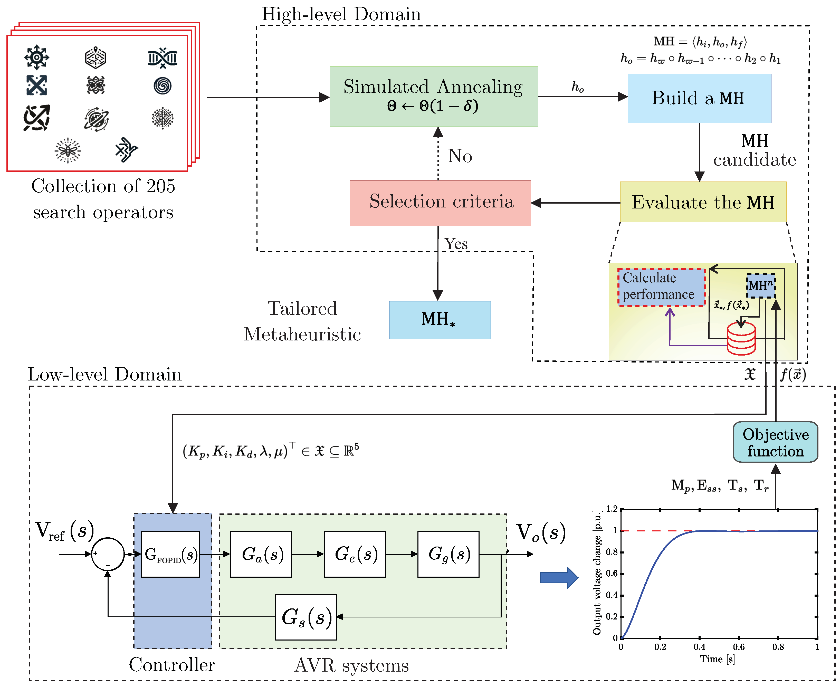
since is the regularization parameter determined after extensive experimentation and predefined as , furthermore, is the penalty value that, for simulation purposes, is 500 when the system is unstable and zero when it is stable. In addition, is the overshoot, is the steady state error, and and are the settling and rise times, respectively. Figure 3 describes this stage in detail.
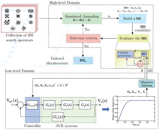
Figure 3.
Automated heuristic-based tuner designing methodology for Fractional-Order PID (FOPID) controllers for Automatic Voltage Regulation (AVR) systems.
During the second stage, our primary objective was to identify the most suitable FOPID configuration for integration with the AVR system. To this end, the FOPID tuning was performed 50 times using the MH achieved in the previous stage, storing the controller constants and their fitness values. This test verified the repeatability of the optimization process, selecting the best FOPID controller obtained in the different replicates.
The last stage was subdivided into three steps. The first step consisted of a comparative analysis with four works published in the literature conceived under similar operating conditions. Table 3 shows the most relevant operating conditions of the works analyzed. In particular, each proposal has a budget and hyper-parameters appropriate to its dynamics. The MHs employed by these works are Cuckoo Search (CS) [17], Particle Swarm Optimization (PSO) [18], Improved Marine Predators Algorithm (MP-SEDA) [19], and Simulated Annealing (SA) [58]. Another point of vital relevance is the objective function, which presents slight variations in each proposal, prioritizing the presence of some additional features (, , , among others). Thus, each proposal shows an objective function configuration, weighting these features using a scaling value or weight. We can observe this in detail in (21), (22), (23), and (24) according to [17], [18], [19], and [58], respectively.
where is the maximum peak time, ITSE is the Integral of Time multiplied by Squared Error Criterion, and ITAE is the Integral of Time multiplied by Absolute Error Criterion. These are metrics of controller performance.
| Algorithm 1 Simulated Annealing Hyper-Heuristic for Automated Metaheuristic Design |
|
Table 3.
Comparison of the features and performance of different metaheuristic approaches as a function of the maximum number of iterations (Max. Iter.), number of sub-iterations (Sub. Iter.), population size (Pop. Size), number of hyper-parameters (Num. HP), number of features for the objective function (Num. Features), and the iterations required for convergence (Conv [Iter]). Where NA is not applicable, the symbol “-” indicates that the information could not be found in the article. “Features” refers to control features such as , , , , among others.
In the second step, we focused on a robustness analysis by perturbing the AVR transfer function. Specifically, a sweep was performed from −50% to 50% variation of the time constants (, , , and ) with an incremental step of 25% for each transfer function composing the AVR (, , , and ). Recall that these variations represent significant changes in the system’s dynamics. Thus, in the last step, we varied fractional orders and between 0.5 and 2 with a step of 0.01 to generate and study two landscapes that detail the overshoot and settling time behavior of the FOPID controller.
All experiments performed in this work were coded in Python v3.9 and ran on an ASUS TUF Gaming F17 with AMD Ryzen 5700G-8 CPU Cores, 16 GB RAM, and Windows 11-64 bit. Also, Matlab R2023b was used to simulate the AVR system; for the FOPID controller, the FOMCON [59] toolbox was utilized. In addition, the freely available CUSTOMHyS framework at PyPI, https://pypi.org/project/customhys/ (accessed on 14 March 2024), was employed to implement the automated heuristic-based tuner designing methodology described above.
4. Numerical Results
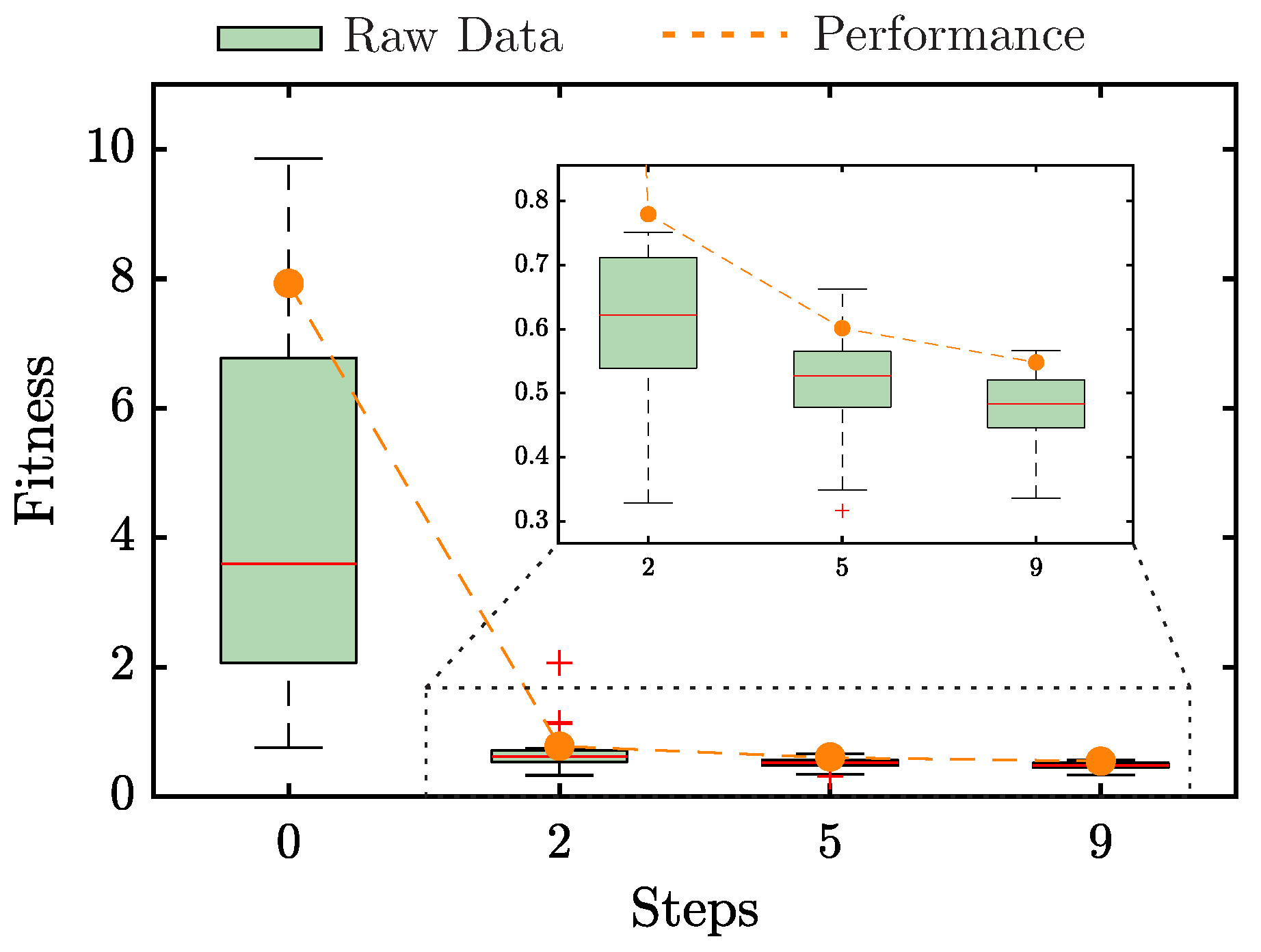
This first stage aims to obtain the MH as it best solves the optimization problem. Figure 4 shows the HH evolution process obtained for this problem. Each boxplot represents the final fitness value for each candidate MH in the replicates to which it was subjected (20 times). In addition, the best performance obtained in the HH process is marked in orange dots. This performance metric is given by Q, presented in (19). The candidate MH went from a value of (step 0) to (step 2), representing an enhancement of 90.17%. Plus, the zoomed box in Figure 4 indicates the steps with a significant improvement. For instance, Q equals 0.61014 at step 5 and decreases to 0.5482 at step 9; these represent 92.30% and 93.08% better values than the initial step, respectively.
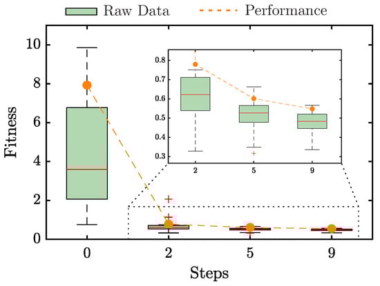
Figure 4.
Evolution of the candidate MH for each hyper-heuristic step. Orange dots and dashed lines illustrate the HH process’s performance.
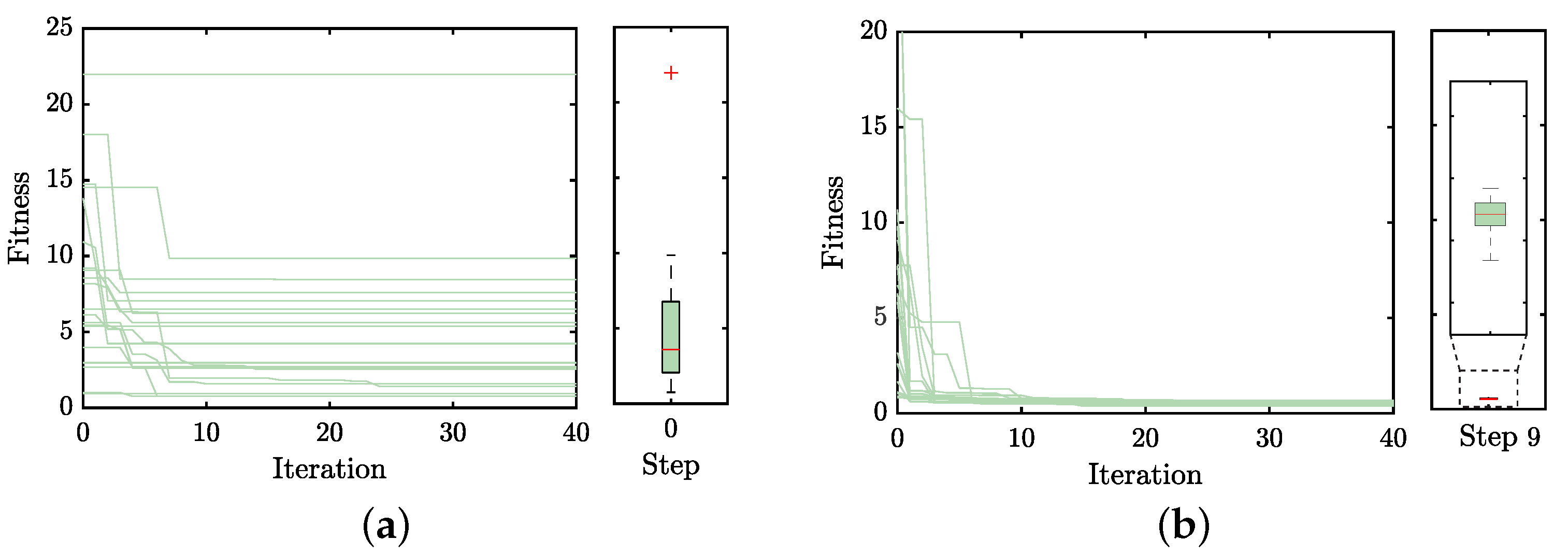
In addition, data collected from steps 0 and 9 were analyzed to compare the performance of the candidate metaheuristics. Figure 5a illustrates the fitness values achieved in step zero, highlighting a noticeable stagnation and significant dispersion in fitness values among the candidate metaheuristics. Conversely, Figure 5b demonstrates that the metaheuristic selected in step 9, denoted as , rapidly converges to a lower fitness value with minimal variation, as evidenced by the corresponding boxplot. It is worth mentioning that the choice of an appropriate MH is crucial in optimization problems due to its significant impact on the efficiency and effectiveness of finding optimal or near-optimal solutions. A well-chosen Metaheuristic can effectively navigate the search space, balancing exploration and exploitation while avoiding early convergence. The problem’s nature, search space characteristics, constraints, and objectives should guide the selection. As demonstrated by our comparison between steps 0 and 9, the right metaheuristic, , can drastically reduce the search time and improve the quality of solutions, emphasizing the significance of a thoughtful and automated selection process.
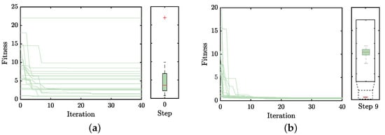
Figure 5.
Fitness evolution obtained by the candidate metaheuristics in the (a) initial and (b) ninth steps during the hyper-heuristic process.
The tailored metaheuristic, denoted as , comprises two distinct perturbation mechanisms. Specifically, the first mechanism is derived from the Swarm Dynamics family, emphasizing collective behavior and information sharing among solutions (i.e., swarm intelligence). The second mechanism arrives from the Genetic Crossover family, which employs biological inheritance and variation principles to generate new solutions. The characteristics and parameters of these perturbators are detailed in Table 4, providing insights into their operational mechanisms and contributions to the efficacy of .
Table 4.
Variation parameters and hyper-parameters of each search operator composing the tailored metaheuristic ().
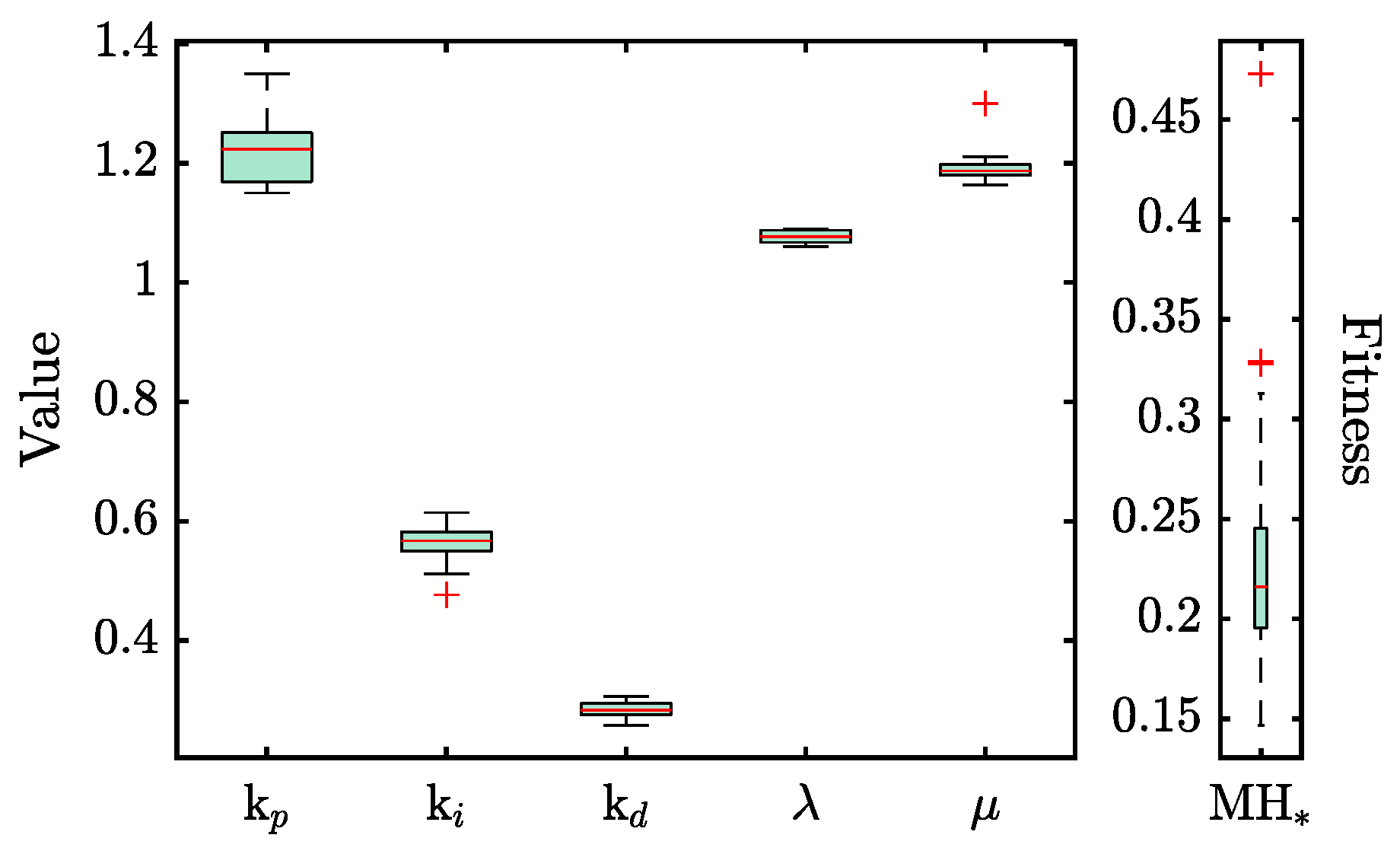
Upon tailoring , its robustness was assessed through a repeatability test to ensure the results’ reliability. Figure 6 depicts boxplots representing the distribution of the FOPID controller’s gains and fractional order variables across 50 iterations of the optimization process. These iterations aimed to verify the consistency of the controller gains and the corresponding fitness values. The results of this experiment emphasize the high repeatability of , with a median fitness performance of 0.216 and a standard deviation of . Such statistical measures indicate a strong reliability in the optimization process under . Furthermore, this evaluation process identified the optimal set of gains that minimized the objective function, specifically targeting improved control features such as peak overshoot (), settling time (), and rise time (). The fine-tuned gains for the FOPID controller are as follows: , , , , and . These delineate the parameters for achieving superior control performance.
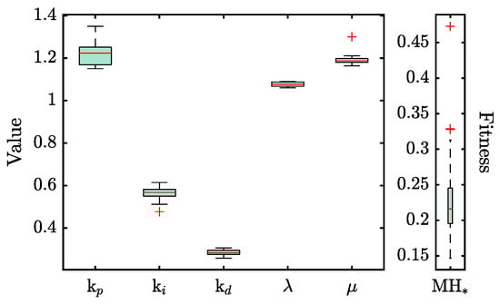
Figure 6.
Distribution of the controller parameters and the resulting fitness values for 50 replicates obtained by .
Table 5 provides a comprehensive comparative analysis between the fine-tuned FOPID controller and four existing approaches, all designed under similar operational conditions for AVR systems and optimized through various MHs. This comparison leverages control gains from studies reported in [17,18,19,58], specifically applied to the case study. The data indicate that our optimization strategy yields a controller performance approximately 1.69 times faster than the comparator approaches, achieving near-zero overshoot. Notably, despite the designed controller exhibiting a rise time that is 2.13 times longer than that reported in [19], it demonstrates the slightest discrepancy between the settling and rise times (), highlighting its efficiency and robustness in dynamic response.
Table 5.
Comparative analysis of the proposed Fractional-Order PID Controller against published approaches in the literature. Colors indicate performance rankings: blue highlights the best values achieved, whereas yellow denotes the least favorable features.
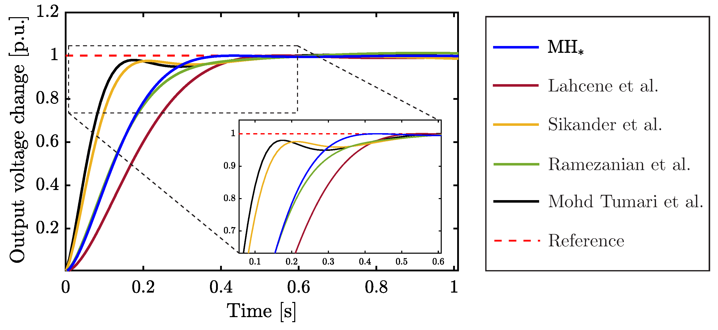
Figure 7 illustrates the dynamic responses of the controllers listed in Table 5, tracking a Heaviside step function. Upon closer examination, it becomes evident that the controller fine-tuned through the tailored MH reaches the steady state with remarkable swiftness, showcasing superior performance. This enhanced response is attributed to the meticulously fine-tuned control gains, as detailed in the third row of Table 5, which significantly improve the system’s transient behavior. Besides, our heuristically tuned controller distinctly outperforms the alternatives in three critical control metrics: peak overshoot (), settling time (), and the difference between settling and rise times (). In comparison, the approach by Sikander et al. [17], represented by the yellow line in the figure, demonstrates the least favorable performance, positioning it at the lower end of the comparative spectrum.
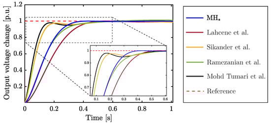
Figure 7.
Step response of different fractional PID controllers designed for the AVR system. The metaheuristic algorithms used to perform the fractional PID controller tuning are: , SA by Lahcene et al. [58], CS by Sikander et al. [17], PSO by Ramezanian et al. [18], and MP-SEDA by Mohd Tumari et al. [19].
On the other hand, this study quantifies the impact of variations in each AVR transfer function parameter (see Table 1) on the performance of the fractional PID controller, as detailed in Table 6. Our analysis covers three critical control features: overshoot, settling time, and rise time (, , and , respectively). To achieve this with incremental steps of 25%, the parameters of the transfer functions were varied within a range of −50% to 50% of their nominal values. It is important to note that the following analysis is conducted individually, i.e., for each AVR transfer function parameter variation. Moreover, these performance impacts are contrasted with the control outcomes achieved through the control gains optimized by the tailored MH (referenced in row 1 of Table 5). Concerning , the overshoot remains at zero for parameter variations of −50% and −25% (as shown in row 3, columns 2 and 3, respectively). However, with a positive increase in this parameter, i.e., at 50% and 75%, the experiences an average increase of 4.71%. Additionally, both and render an average increase of 1.86 and 1.09 times, respectively, irrespective of the variation in .
Table 6.
Comparative analysis of the proposed fractional PID controller performance across a range of variations in AVR transfer function parameters. , , , and denote the parameters for the amplifier, exciter, generator, and sensor models, respectively, as detailed in Table 1.
A similar trend is observed with , where equals zero for negative variations but experiences an average increase of 3.97% for positive changes. Likewise, the values indicate that the proposed controller response becomes 66.50% slower before achieving a steady state. Interestingly, negative variations in lead to faster rise times, whereas positive ones result in slower rise times.
In the case of , this parameter consistently influences the overshoot across all variations, resulting in an average increment of 2.46% for this control feature. Moreover, this parameter significantly delays the control response, effectively tripling the settling time. Similarly, impacts the rise time, where negative changes reduce it (as detailed in row 12, columns 2 and 3), and positive changes cause it to increase by 1.36 times (as seen in row 12, columns 4 and 6). With respect to , it is noteworthy that negative fluctuations maintain overshoots at zero and induce only slight variations in either the settling or rise times. In contrast, positive variations lead to increments of 0.51% for the overshoot and reductions of 5.74% and 1.65% for the settling and rise times, respectively.
The analysis reveals that the most affected control feature is , specifically at the opposite extremes of the transfer function parameters variation (±50%, as shown in columns 2 and 5). The least compromised AVR transfer function is associated with the sensor model ( parameter), likely due to the relatively minor variations observed compared to the other parameters. Despite this, the performance of the fine-tuned controller still demonstrates superior efficiency compared to some approaches detailed in Table 5, highlighting its robustness across a broad range of operational conditions.
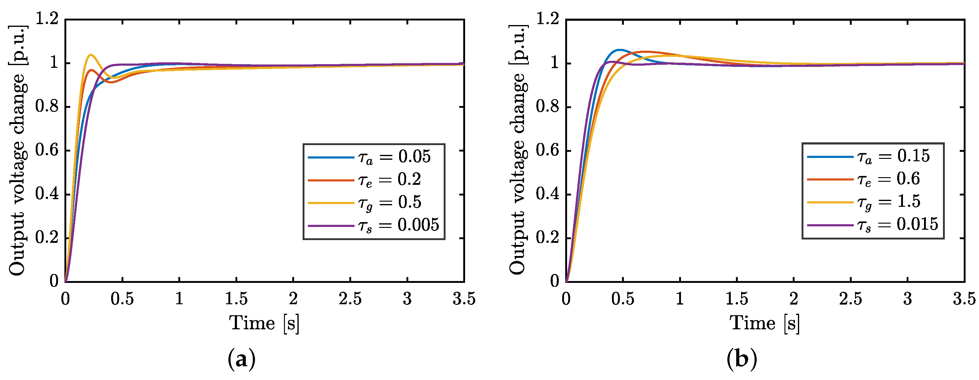
Figure 8a,b depict the performance of the fractional PID controller under parameter variations for each of the AVR transfer functions. For the sake of clarity and practicality, only variations of −50% and 50% are presented, as they exemplify the most significant effects on the control performance. The controller fine-tuned via the tailored metaheuristic demonstrates consistent robustness and stability across the varied disturbance conditions analyzed in this work.
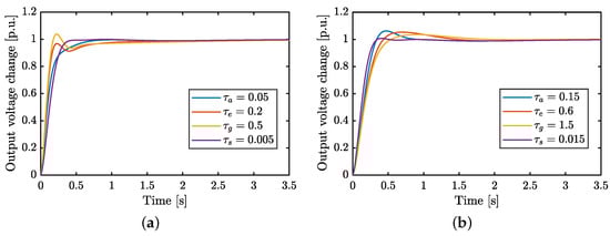
Figure 8.
Step responses of the fine-tuned Fractional-Order PID controller under parameter variations of (a) −50% and (b) 50% for each AVR transfer function. , , , and represent the parameters of the amplifier, exciter, generator, and sensor models, respectively (see Table 1).
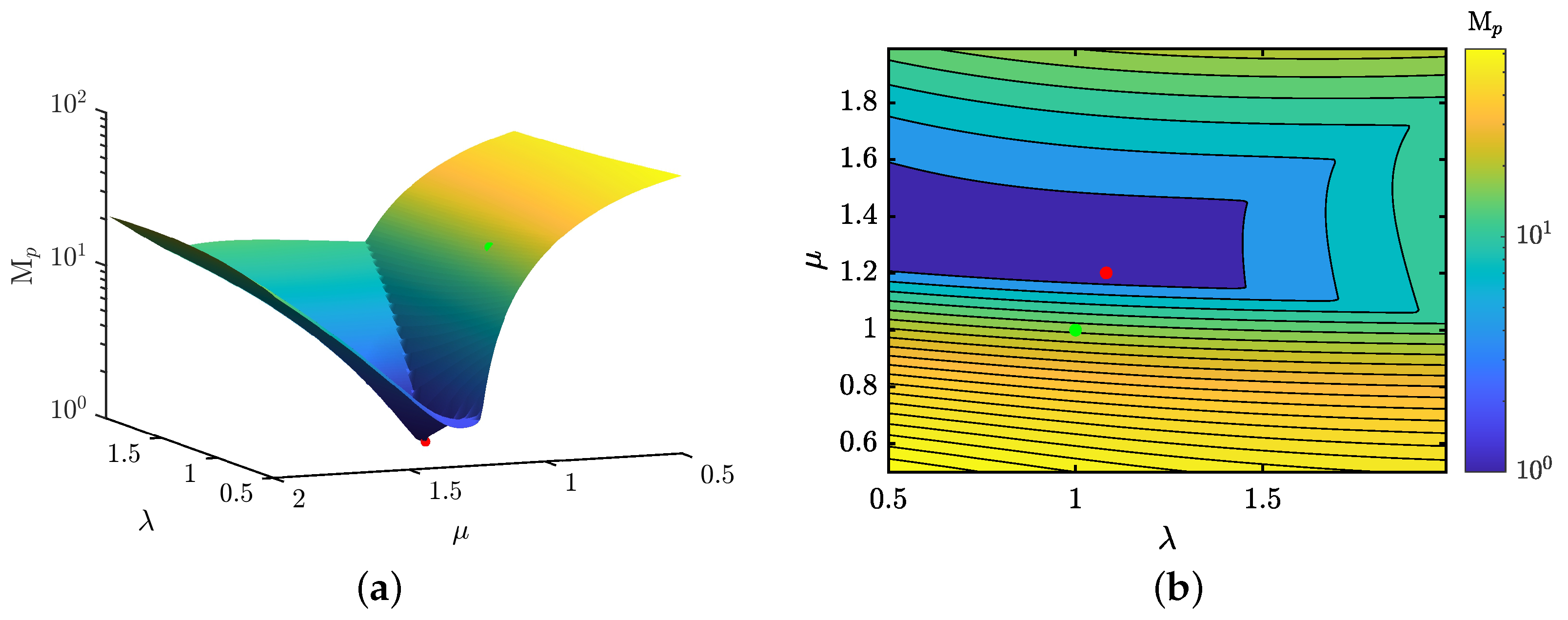
Figure 9 and Figure 10 illustrate the relationship between the fractional parameters and , and their impact on two critical control features, and . These contour maps enable the identification of - combinations that minimize or maximize the overshoot and settling time of the AVR system, with darker colors indicating lower values and lighter colors higher values of these control features. The green marker highlights the minimum and values achieved by the standard PID structure, whereas the red marker signifies the outcomes obtained with the fractional control scheme (referenced in row 1 of Table 5).
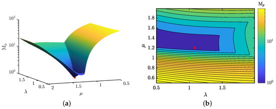
Figure 9.
Landscape of relationship and and their effects over the overshoot: (a) Isometric view of the overshoot landscape; and (b) Superior view of the overshoot landscape.
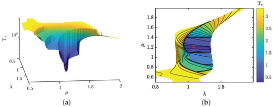
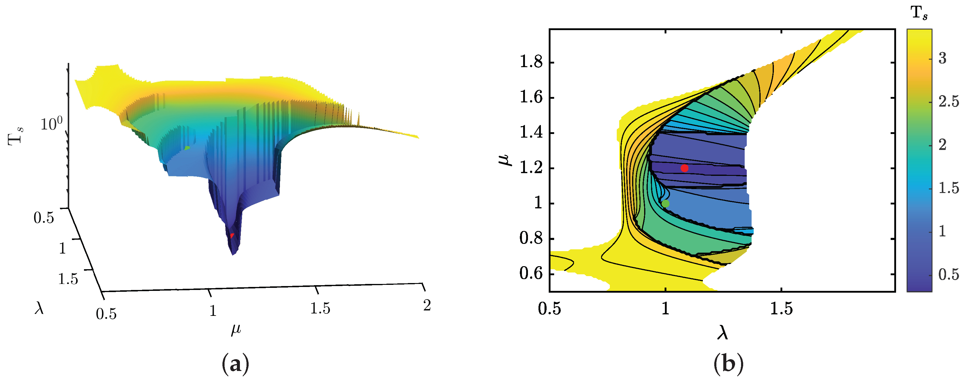
Figure 10.
Landscape of relationship and and their effects over the settling time: (a) Isometric view of the settling time landscape; and (b) Superior view of the settling time landscape.
The analysis reveals that spans a wide range from 0% to 64%, while fluctuates within a more confined spectrum, between 0.33 s and 3.49 s. These plots demarcate reliable regions for stable AVR system operation concerning these control features.
Aiming to refine significantly the transitory response over the traditional PID control (denoted by the green point)—specifically, to reduce overshoot and settling time—the blue regions in these plots are especially targeted. The tailored MH and the proposed fitness criterion suggest a pivotal relationship for the fractional parameters: is essential for attaining the optimal response. It becomes apparent that the optimal - combination can render the controller four times faster with zero overshoot compared to the traditional PID, which exhibits control features of = 1.34 s and . In summary, integrating fractional calculus into PID control introduces a higher degree of complexity in gain tuning. Nonetheless, this approach significantly enhances the robustness of AVR dynamics, offering a wider spectrum of feasible control features.
5. Conclusions
In this work, we implemented a methodology based on Automated Algorithm Design (AAD), focusing on Metaheuristic (MH) design for engineering applications. A perturbative selection hyper-heuristic model, driven by Simulated Annealing, was employed to construct a tailored metaheuristic (). The design of involved a specific sequence of search operators: an inertial swarm dynamic perturbator followed by a metropolis selector, and a crossover genetic operator succeeded again by a metropolis selection. As a case study, a Fractional-Order Proportional-Integral-Derivative (FOPID) controller was fine-tuned through to enhance the Automatic Voltage Regulator (AVR) response.
The comparative analysis demonstrated that the FOPID controller, fine-tuned via , exhibited superior control features compared to similar approaches documented in the literature, such as improved settling time and reduced overshoot. On average, the achieved controller delivered responses 1.69 times faster with virtually no overshoots. Furthermore, variations within each subsystem of the AVR plant were tested to assess the controller’s robustness in terms of these control features. The greatest and least settling times were observed when (corresponding to the generator subsystem) experienced perturbations at the extreme ranges of −50% and 50% of its nominal value, respectively. Regarding overshoot, this feature remained near zero for negative variations of the , , and parameters (amplifier, exciter, and sensor subsystems, respectively). However, when these parameters were perturbed to 50% of their nominal values, they exhibited an average overshoot of 6.219%.
Additionally, a landscape analysis focusing on these control features was conducted by maintaining the gains , , and constant while varying and . This analysis enabled the identification of controller settings that offered overshoots and settling times within the range of 0% to 64% and 0.33 s to 3.49 s, respectively, indicating that incorporating the fractional domain into conventional control schemes expands the AVR system’s control gain possibilities. However, these degrees of freedom were limited, as evidenced by the settling time landscape, where the stability region was clearly defined.
Although this study focused on a specific problem, the proposed AAD methodology holds the potential to guide practitioners toward achieving suitable performance on a broader array of optimization problems. Future research aims to extend this approach to other real-world engineering applications, evaluating the effectiveness of customized MHs in scenarios akin to design specifications.
Author Contributions
Conceptualization, D.F.Z.-G.; Formal analysis, J.M.C.-D. and J.G.A.-C.; Investigation, D.F.Z.-G., G.H.V.-R., I.A., J.M.C.-D. and J.G.A.-C.; Methodology, D.F.Z.-G., G.H.V.-R., I.A., J.M.C.-D. and J.G.A.-C.; software, D.F.Z.-G. and J.M.C.-D.; Validation, J.M.C.-D., I.A. and J.G.A.-C.; Writing—original draft, D.F.Z.-G. and G.H.V.-R.; writing—review and editing, D.F.Z.-G., G.H.V.-R., I.A., J.M.C.-D. and J.G.A.-C. All authors have read and agreed to the published version of the manuscript.
Funding
This work was supported by the Research Group in Advanced Artificial Intelligence at Tecnologico de Monterrey, grant NUA A00836756 and A00834075, and the Mexican Council of Humanities, Sciences, and Technologies (CONAHCyT) under scholarships 1046000 and 863547. Besides, this work was partly supported by the University of Guanajuato through CIIC (Convocatoria Institucional de Investigación Científica, UG) Project 243/2024.
Institutional Review Board Statement
Not required for this study.
Informed Consent Statement
No Formal written consent was required for this study.
Data Availability Statement
Data available under a formal demand.
Conflicts of Interest
All authors declare no conflicts of interest in this paper.
References
- Al-Shetwi, A.Q.; Hannan, M.; Jern, K.P.; Mansur, M.; Mahlia, T.M.I. Grid-connected renewable energy sources: Review of the recent integration requirements and control methods. J. Clean. Prod. 2020, 253, 119831. [Google Scholar] [CrossRef]
- Andersson, G.; Bel, C.Á.; Cañizares, C. Frequency and voltage control. In Electric Energy Systems; CRC Press: Boca Raton, FL, USA, 2017; pp. 355–400. [Google Scholar]
- Ji, Y.; He, W.; Cheng, S.; Kurths, J.; Zhan, M. Dynamic network characteristics of power-electronics-based power systems. Sci. Rep. 2020, 10, 9946. [Google Scholar] [CrossRef] [PubMed]
- Perera, S.; Elphick, S. Chapter 7—Implications of equipment behaviour on power quality. In Applied Power Quality; Perera, S., Elphick, S., Eds.; Elsevier: Amsterdam, The Netherlands, 2023; pp. 185–258. [Google Scholar] [CrossRef]
- Karaagac, U.; Kocar, I.; Mahseredjian, J.; Cai, L.; Javid, Z. STATCOM integration into a DFIG-based wind park for reactive power compensation and its impact on wind park high voltage ride-through capability. Electr. Power Syst. Res. 2021, 199, 107368. [Google Scholar] [CrossRef]
- Ćalasan, M.; Kecojević, K.; Lukačević, O.; Ali, Z.M. Chapter 10—Testing of influence of SVC and energy storage device’s location on power system using GAMS. In Uncertainties in Modern Power Systems; Zobaa, A.F., Abdel Aleem, S.H., Eds.; Academic Press: Cambridge, MA, USA, 2021; pp. 297–342. [Google Scholar] [CrossRef]
- Abood, L.H.; Oleiwi, B.K. Design of fractional order PID controller for AVR system using whale optimization algorithm. Indones. J. Electr. Eng. Comput. Sci. 2021, 23, 1410–1418. [Google Scholar] [CrossRef]
- Köse, E. Optimal control of AVR system with tree seed algorithm-based PID controller. IEEE Access 2020, 8, 89457–89467. [Google Scholar] [CrossRef]
- Jahanshahi, E.; Sivalingam, S.; Schofield, J.B. Industrial test setup for autotuning of PID controllers in large-scale processes: Applied to Tennessee Eastman process. IFAC-PapersOnLine 2015, 48, 469–476. [Google Scholar] [CrossRef]
- Shah, P.; Agashe, S. Review of fractional PID controller. Mechatronics 2016, 38, 29–41. [Google Scholar] [CrossRef]
- Izci, D.; Ekinci, S.; Mirjalili, S. Optimal PID plus second-order derivative controller design for AVR system using a modified Runge Kutta optimizer and Bode’s ideal reference model. Int. J. Dyn. Control 2023, 11, 1247–1264. [Google Scholar] [CrossRef]
- Sivanandhan, A.; Aneesh, V. A Hybrid Technique Linked FOPID for a Nonlinear System Based On Closed-Loop Settling Time of Plant. Robot. Auton. Syst. 2024, 176, 104651. [Google Scholar] [CrossRef]
- Podlubny, I. Fractional-order systems and fractional-order controllers. Inst. Exp. Phys. Slovak Acad. Sci. Kosice 1994, 12, 1–18. [Google Scholar]
- Izci, D.; Ekinci, S.; Hekimoğlu, B. Fractional-order PID controller design for buck converter system via hybrid Lévy flight distribution and simulated annealing algorithm. Arab. J. Sci. Eng. 2022, 47, 13729–13747. [Google Scholar] [CrossRef]
- Nassef, A.M.; Abdelkareem, M.A.; Maghrabie, H.M.; Baroutaji, A. Metaheuristic-Based Algorithms for Optimizing Fractional-Order Controllers—A Recent, Systematic, and Comprehensive Review. Fractal Fract. 2023, 7, 553. [Google Scholar] [CrossRef]
- Altbawi, S.M.A.; Mokhtar, A.S.B.; Jumani, T.A.; Khan, I.; Hamadneh, N.N.; Khan, A. Optimal design of Fractional order PID controller based Automatic voltage regulator system using gradient-based optimization algorithm. J. King Saud Univ.-Eng. Sci. 2021, 36, 32–44. [Google Scholar] [CrossRef]
- Sikander, A.; Thakur, P.; Bansal, R.C.; Rajasekar, S. A novel technique to design cuckoo search based FOPID controller for AVR in power systems. Comput. Electr. Eng. 2018, 70, 261–274. [Google Scholar] [CrossRef]
- Ramezanian, H.; Balochian, S.; Zare, A. Design of optimal fractional-order PID controllers using particle swarm optimization algorithm for automatic voltage regulator (AVR) system. J. Control. Autom. Electr. Syst. 2013, 24, 601–611. [Google Scholar] [CrossRef]
- Mohd Tumari, M.Z.; Ahmad, M.A.; Suid, M.H.; Hao, M.R. An improved marine predators algorithm-tuned fractional-order PID controller for automatic voltage regulator system. Fractal Fract. 2023, 7, 561. [Google Scholar] [CrossRef]
- Srinivas, M.; Patnaik, L.M. Genetic algorithms: A survey. Computer 1994, 27, 17–26. [Google Scholar] [CrossRef]
- Price, K.; Storn, R.M.; Lampinen, J.A. Differential Evolution: A Practical Approach to Global Optimization; Springer Science & Business Media: Berlin/Heidelberg, Germany, 2006. [Google Scholar] [CrossRef]
- Kennedy, J.; Eberhart, R. Particle swarm optimization (PSO). In Proceedings of the International Conference on Neural Networks (ICNN’95), Perth, WA, Australia, 27 November–1 December 1995; Volume 4, pp. 1942–1948. [Google Scholar]
- de Armas, J.; Lalla-Ruiz, E.; Tilahun, S.L.; Voß, S. Similarity in metaheuristics: A gentle step towards a comparison methodology. Nat. Comput. 2022, 21, 265–287. [Google Scholar] [CrossRef]
- Tzanetos, A.; Dounias, G. Nature inspired optimization algorithms or simply variations of metaheuristics? Artif. Intell. Rev. 2021, 54, 1841–1862. [Google Scholar] [CrossRef]
- Piotrowski, A.P.; Napiorkowski, J.J.; Rowinski, P.M. How novel is the “novel” black hole optimization approach? Inf. Sci. 2014, 267, 191–200. [Google Scholar] [CrossRef]
- Stützle, T.; López-Ibáñez, M. Automated design of metaheuristic algorithms. In Handbook of Metaheuristics; Springer: Berlin/Heidelberg, Germany, 2019; pp. 541–579. [Google Scholar]
- Yi, W.; Qu, R.; Jiao, L.; Niu, B. Automated Design of Metaheuristics Using Reinforcement Learning Within a Novel General Search Framework. IEEE Trans. Evol. Comput. 2023, 27, 1072–1084. [Google Scholar] [CrossRef]
- Hassan, A.; Pillay, N. Hybrid metaheuristics: An automated approach. Expert Syst. Appl. 2019, 130, 132–144. [Google Scholar] [CrossRef]
- Qu, R.; Kendall, G.; Pillay, N. The General Combinatorial Optimisation Problem: Towards Automated Algorithm Design. IEEE Comput. Intell. Mag. 2020, 15, 14–23. [Google Scholar] [CrossRef]
- Cruz-Duarte, J.; Amaya, I.; Ortiz-Bayliss, J.; Conant-Pablos, S.; Terashima-Marín, H.; Shi, Y. Hyper-Heuristics to customise metaheuristics for continuous optimisation. Swarm Evol. Comput. 2021, 66, 100935. [Google Scholar] [CrossRef]
- Burke, E.K.; Gendreau, M.; Hyde, M.; Kendall, G.; Ochoa, G.; Özcan, E.; Qu, R. Hyper-heuristics: A survey of the state of the art. J. Oper. Res. Soc. 2013, 64, 1695–1724. [Google Scholar] [CrossRef]
- Zambrano-Gutierrez, D.F.; Cruz-Duarte, J.M.; Avina-Cervantes, J.G.; Ortiz-Bayliss, J.C.; Yanez-Borjas, J.J.; Amaya, I. Automatic Design of Metaheuristics for Practical Engineering Applications. IEEE Access 2023, 11, 7262–7276. [Google Scholar] [CrossRef]
- Patil, P.M.; Patil, S. Automatic voltage regulator. In Proceedings of the 2020 International Conference on Emerging Trends in Information Technology and Engineering (ic-ETITE), Vellore, India, 24–25 February 2020; pp. 1–5. [Google Scholar]
- Yoshida, H.; Kawata, K.; Fukuyama, Y.; Takayama, S.; Nakanishi, Y. A particle swarm optimization for reactive power and voltage control considering voltage security assessment. IEEE Trans. Power Syst. 2000, 15, 1232–1239. [Google Scholar] [CrossRef]
- Podlubny, I. Fractional Differential Equations: An Introduction to Fractional Derivatives, Fractional Differential Equations, to Methods of Their Solution and Some of Their Applications; Elsevier: Amsterdam, The Netherlands, 1998. [Google Scholar]
- Chen, Y.; Petras, I.; Xue, D. Fractional order control—A tutorial. In Proceedings of the 2009 American Control Conference, St. Louis, MO, USA, 10–12 June 2009; pp. 1397–1411. [Google Scholar] [CrossRef]
- Loverro, A. Fractional Calculus: History, Definitions and Applications for the Engineer. Rapport Technique, Univeristy of Notre Dame: Department of Aerospace and Mechanical Engineering. 2004, pp. 1–28. Available online: https://citeseerx.ist.psu.edu/document?repid=rep1&type=pdf&doi=6256fee0c10bdb7096df51ca8e64df58414ed026 (accessed on 5 January 2024).
- Monje, C.A.; Chen, Y.; Vinagre, B.M.; Xue, D.; Feliu-Batlle, V. Fractional-Order Systems and Controls: Fundamentals and Applications; Springer Science & Business Media: Berlin/Heidelberg, Germany, 2010. [Google Scholar]
- Caputo, M. Linear models of dissipation whose Q is almost frequency independent—II. Geophys. J. Int. 1967, 13, 529–539. [Google Scholar] [CrossRef]
- Ortigueira, M.D. Principles of fractional signal processing. Digit. Signal Process. 2024, 149, 104490. [Google Scholar] [CrossRef]
- Sun, H.; Chang, A.; Zhang, Y.; Chen, W. A review on variable-order fractional differential equations: Mathematical foundations, physical models, numerical methods and applications. Fract. Calc. Appl. Anal. 2019, 22, 27–59. [Google Scholar] [CrossRef]
- Joseph, S.B.; Dada, E.G.; Abidemi, A.; Oyewola, D.O.; Khammas, B.M. Metaheuristic algorithms for PID controller parameters tuning: Review, approaches and open problems. Heliyon 2022, 8, E09399. [Google Scholar] [CrossRef]
- Ersali, C.; Hekimoğlu, B. A novel opposition-based hybrid cooperation search algorithm with Nelder–Mead for tuning of FOPID-controlled buck converter. Trans. Inst. Meas. Control 2024, 1–19. [Google Scholar] [CrossRef]
- Tejado, I.; Vinagre, B.M.; Traver, J.E.; Prieto-Arranz, J.; Nuevo-Gallardo, C. Back to basics: Meaning of the parameters of fractional order PID controllers. Mathematics 2019, 7, 530. [Google Scholar] [CrossRef]
- Can Kurucu, M.; Yumuk, E.; Güzelkaya, M.; Eksin, I. Online tuning of derivative order term of variable-order fractional proportional–integral–derivative controllers for the first-order time delay systems. Asian J. Control 2023, 25, 2628–2640. [Google Scholar] [CrossRef]
- Chen, X.; Wang, C.; Xu, J.; Long, S.; Chai, F.; Li, W.; Song, X.; Wang, X.; Wan, Z. Membrane humidity control of proton exchange membrane fuel cell system using fractional-order PID strategy. Appl. Energy 2023, 343, 8–13. [Google Scholar] [CrossRef]
- Hussain, K.; Salleh, M.N.M.; Cheng, S.; Shi, Y. Metaheuristic research: A comprehensive survey. Artif. Intell. Rev. 2019, 52, 2191–2233. [Google Scholar] [CrossRef]
- Abdel-Basset, M.; Abdel-Fatah, L.; Sangaiah, A.K. Chapter 10—Metaheuristic Algorithms: A Comprehensive Review. In Computational Intelligence for Multimedia Big Data on the Cloud with Engineering Applications; Intelligent Data-Centric Systems; Academic Press: Cambridge, MA, USA, 2018; pp. 185–231. [Google Scholar] [CrossRef]
- Sörensen, K. Metaheuristics—The metaphor exposed. Int. Trans. Oper. Res. 2015, 22, 3–18. [Google Scholar] [CrossRef]
- Cruz-Duarte, J.; Ortiz-Bayliss, J.; Amaya, I.; Shi, Y.; Terashima-Marín, H.; Pillay, N. Towards a Generalised Metaheuristic Model for Continuous Optimisation Problems. Mathematics 2020, 8, 2046. [Google Scholar] [CrossRef]
- Pillay, N.; Qu, R. Hyper-Heuristics: Theory and Applications; Springer: Berlin/Heidelberg, Germany, 2018. [Google Scholar]
- Kramer, O.; Kramer, O. Genetic Algorithms; Springer: Berlin/Heidelberg, Germany, 2017. [Google Scholar]
- Cruz-Duarte, J.M.; Amaya, I.; Ortiz-Bayliss, J.C.; Terashima-Marín, H.; Shi, Y. CUSTOMHyS: Customising Optimisation Metaheuristics via Hyper-heuristic Search. SoftwareX 2020, 12, 100628. [Google Scholar] [CrossRef]
- Alfaro-Fernández, P.; Ruiz, R.; Pagnozzi, F.; Stützle, T. Automatic algorithm design for hybrid flowshop scheduling problems. Eur. J. Oper. Res. 2020, 282, 835–845. [Google Scholar] [CrossRef]
- López-Ibáñez, M.; Dubois-Lacoste, J.; Cáceres, L.P.; Birattari, M.; Stützle, T. The irace package: Iterated racing for automatic algorithm configuration. Oper. Res. Perspect. 2016, 3, 43–58. [Google Scholar] [CrossRef]
- Zhao, Q.; Duan, Q.; Yan, B.; Cheng, S.; Shi, Y. Automated Design of Metaheuristic Algorithms: A Survey. arXiv 2023, arXiv:2303.06532. [Google Scholar]
- Drake, J.H.; Kheiri, A.; Özcan, E.; Burke, E.K. Recent advances in selection hyper-heuristics. Eur. J. Oper. Res. 2020, 285, 405–428. [Google Scholar] [CrossRef]
- Lahcene, R.; Abdeldjalil, S.; Aissa, K. Optimal tuning of fractional order PID controller for AVR system using simulated annealing optimization algorithm. In Proceedings of the 2017 5th International Conference on Electrical Engineering—Boumerdes (ICEE-B), Boumerdes, Algeria, 29–31 October 2017; pp. 1–6. [Google Scholar] [CrossRef]
- Tepljakov, A.; Tepljakov, A. FOMCON: Fractional-order modeling and control toolbox. In Fractional-Order Modeling and Control of Dynamic Systems; Springer: Cham, Switzerland, 2017; pp. 107–129. [Google Scholar]

Disclaimer/Publisher’s Note: The statements, opinions and data contained in all publications are solely those of the individual author(s) and contributor(s) and not of MDPI and/or the editor(s). MDPI and/or the editor(s) disclaim responsibility for any injury to people or property resulting from any ideas, methods, instructions or products referred to in the content. |
© 2024 by the authors. Licensee MDPI, Basel, Switzerland. This article is an open access article distributed under the terms and conditions of the Creative Commons Attribution (CC BY) license (https://creativecommons.org/licenses/by/4.0/).