
Fractal-Based Multi-Criteria Feature Selection to Enhance Predictive Capability of AI-Driven Mineral Prospectivity Mapping

 ,
,
Abstract
1. Introduction
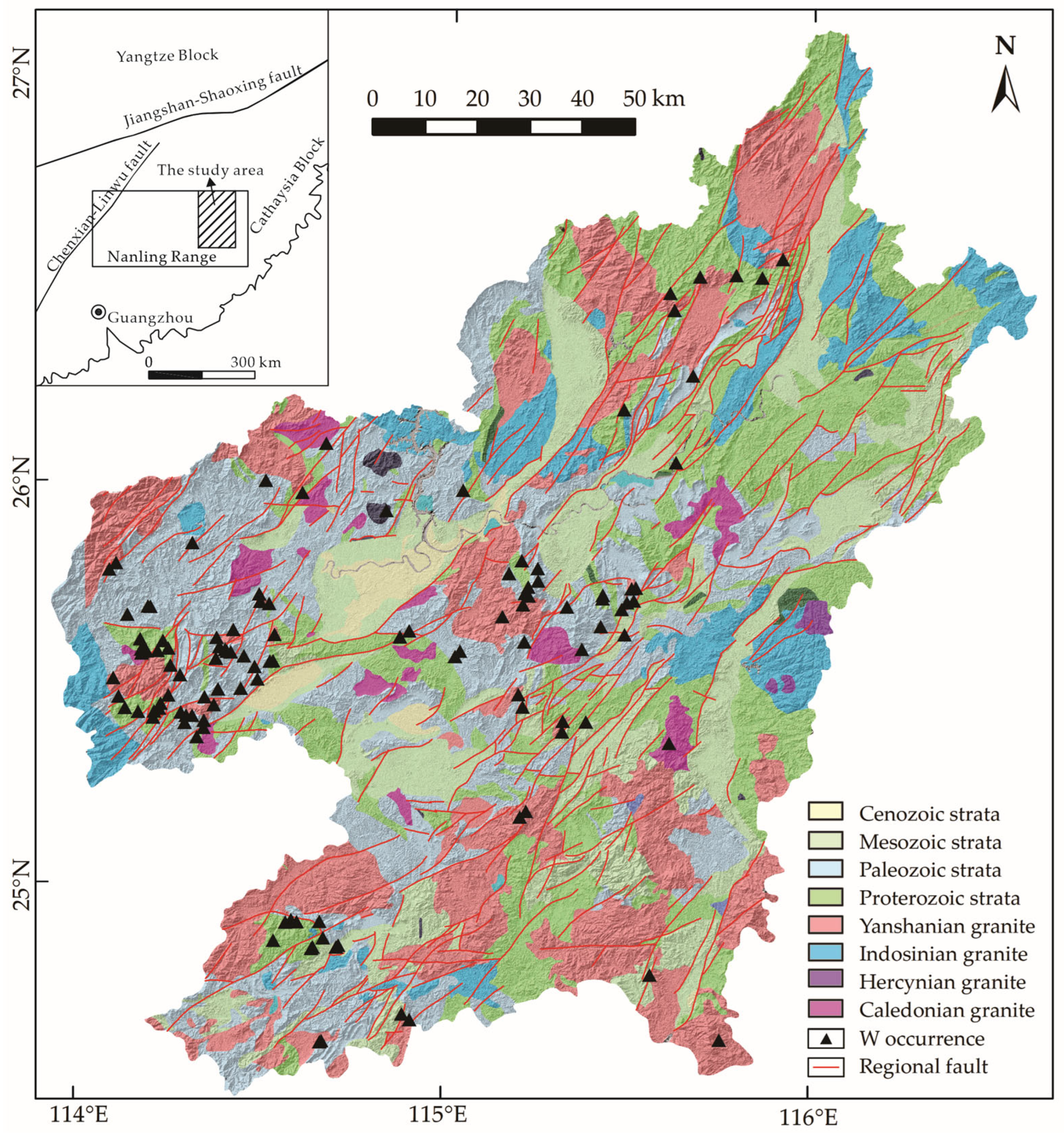
2. Study Area and Data Used
3. Methods
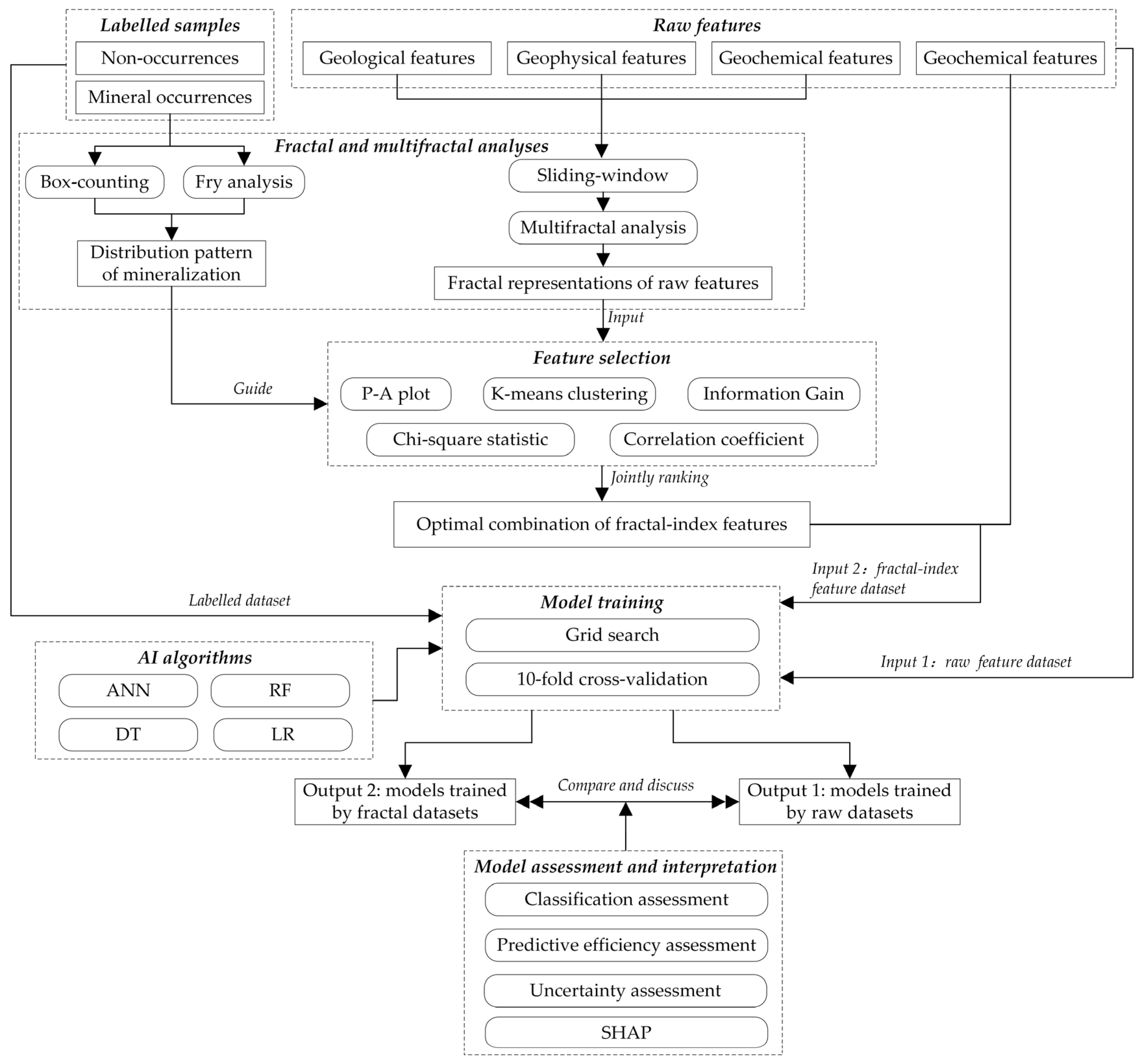
3.1. Proposed Framework
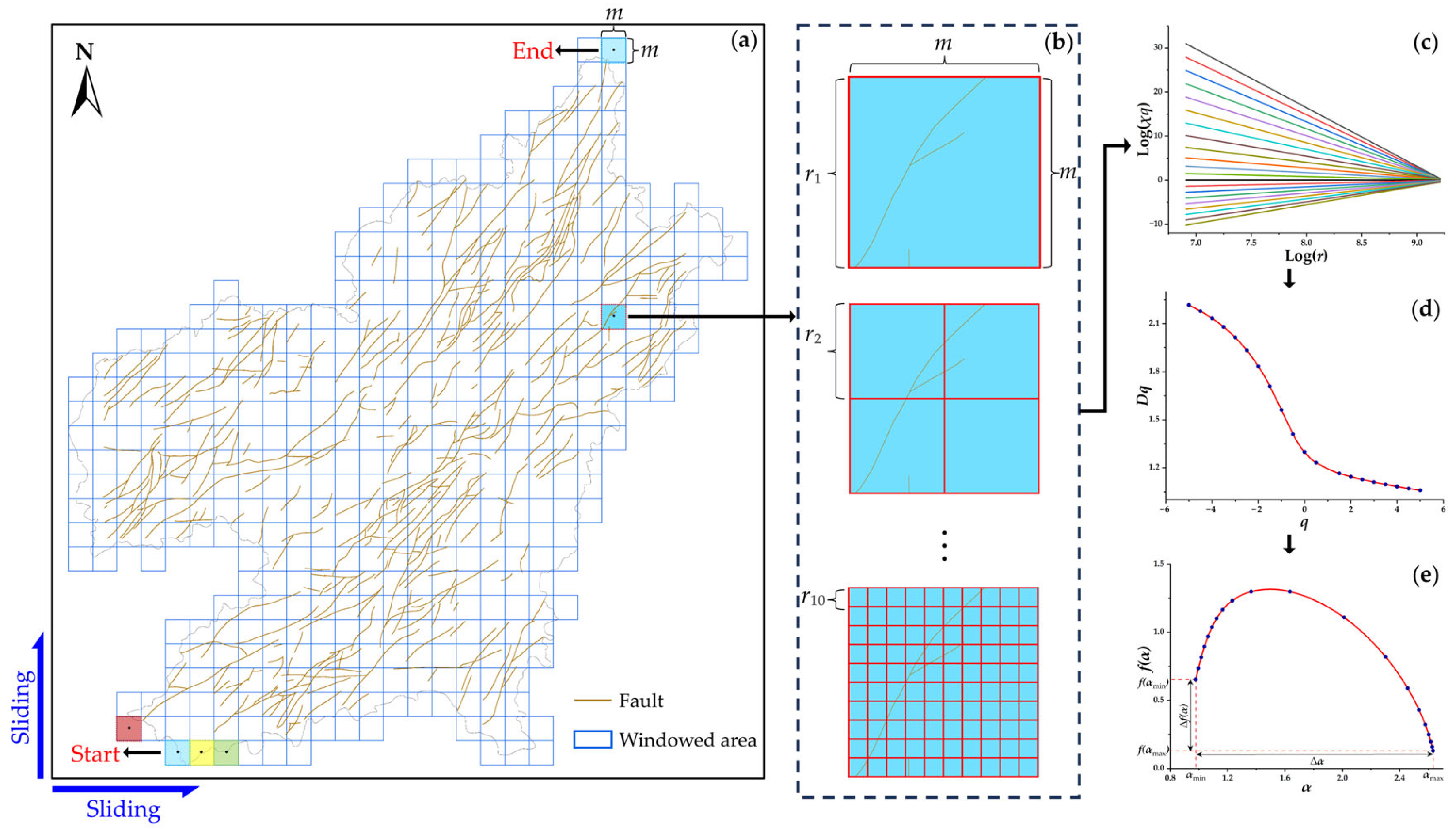
3.2. Fractal and Multifractal Methods
| Algorithm 1: Implementation of multifractal calculation based on sliding window |
| Input: Evidence layer L, center-of-mass coordinate set S, window length m, list of q values Q, list of r values R. |
| Output: Capacity dimension D0, information dimension D1, correlation dimension D2, spectral width ∆α, and spectral height ∆f(α) for the evidence layer. |
| Procedure: Window starts from the bottom-left corner of L. Slide right first, then slide up. Window ends at the upper-right corner of L. Calculate partition function χq, mass exponent τq, and generalized fractal dimension Dq. |
| for row in S do center_x = row [0] center_y = row [1] w_length = m w_position←[center_x, center_y] window←Create(w_length, w_position) a = Intersection_region(window, L) for r in R do p←number(element)/total_number(window) Save[P]←p χq←(P, Q), τq←(χq, R), Dq←(R, χq, Q) if q==0 then D0 = Dq=0 if q==1 then D1 = Dq=1 if q==2 then D2 = Dq=2 α(q) = dDq/dq, f(α) = qα − τq, Δα = αmax − αmin, Δf(α) = f(αmin) − f(αmax) Save[A]←(a: D0, D1, D2, ∆α, ∆f(α)) Output[A] end |
3.3. Criteria for Feature Selection
3.4. AI-Driven MPM
3.4.1. Machine Learning Algorithms
3.4.2. Performance Metrics
3.5. Implementation of the Proposed Framework
4. Results
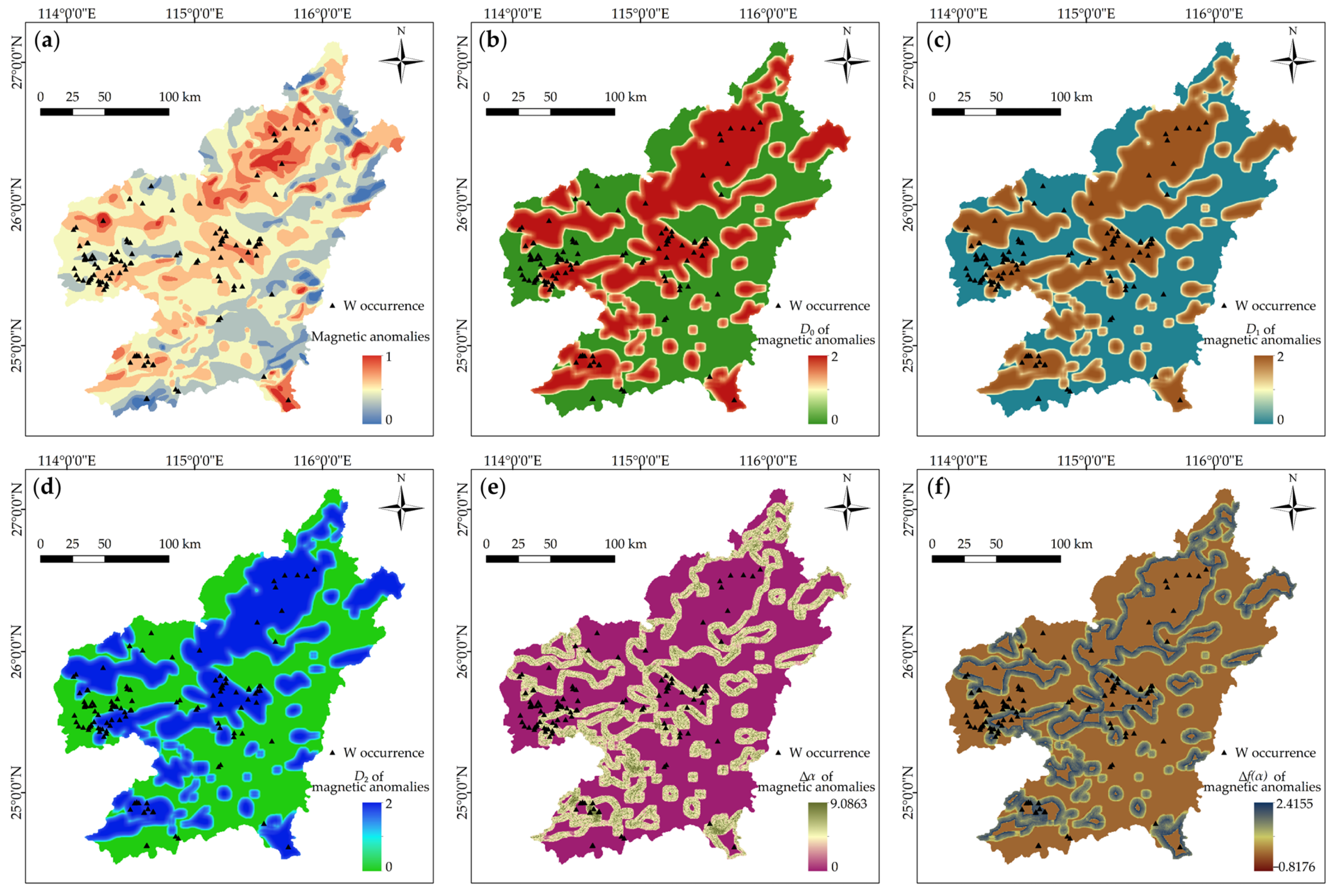
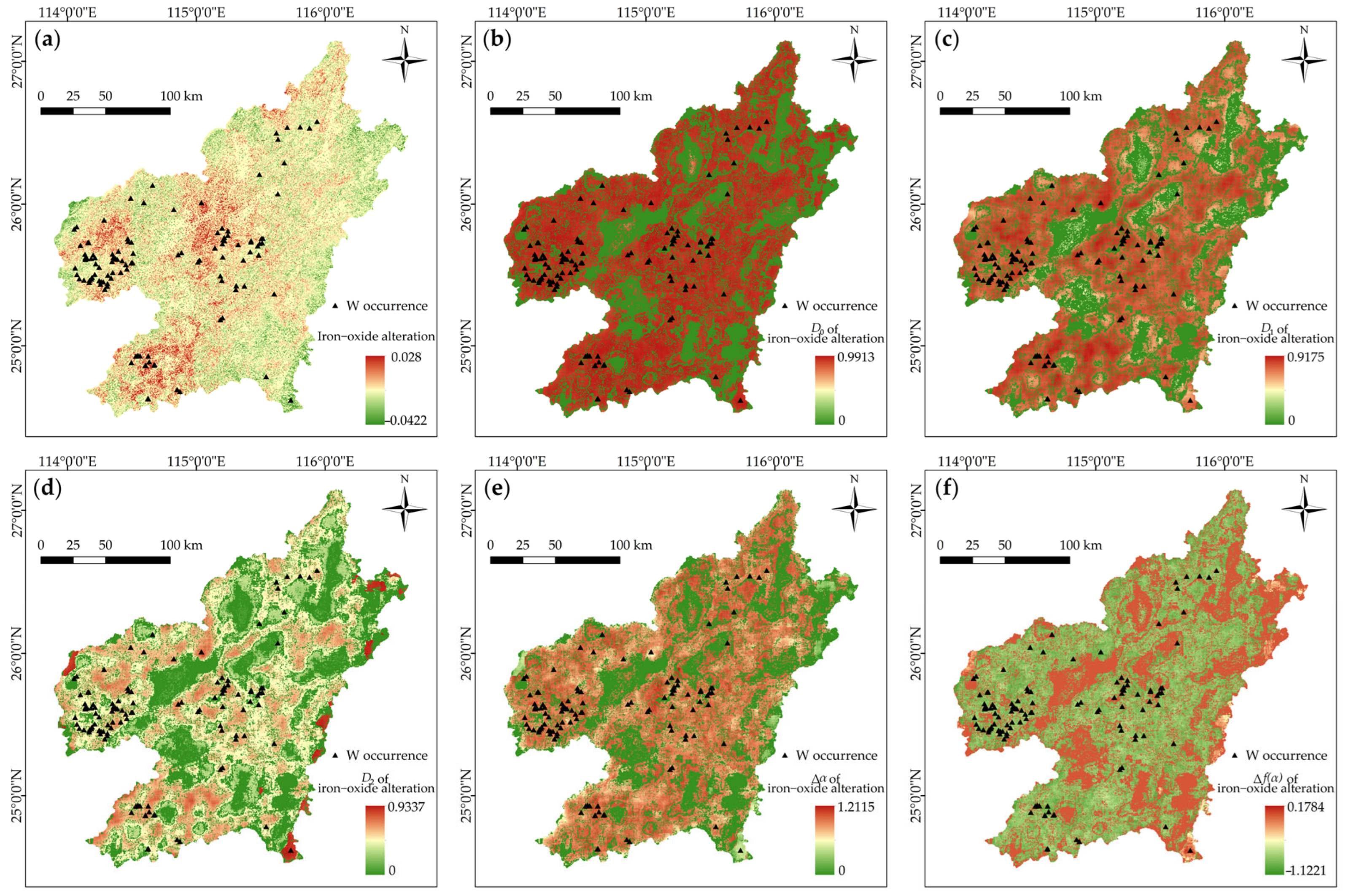
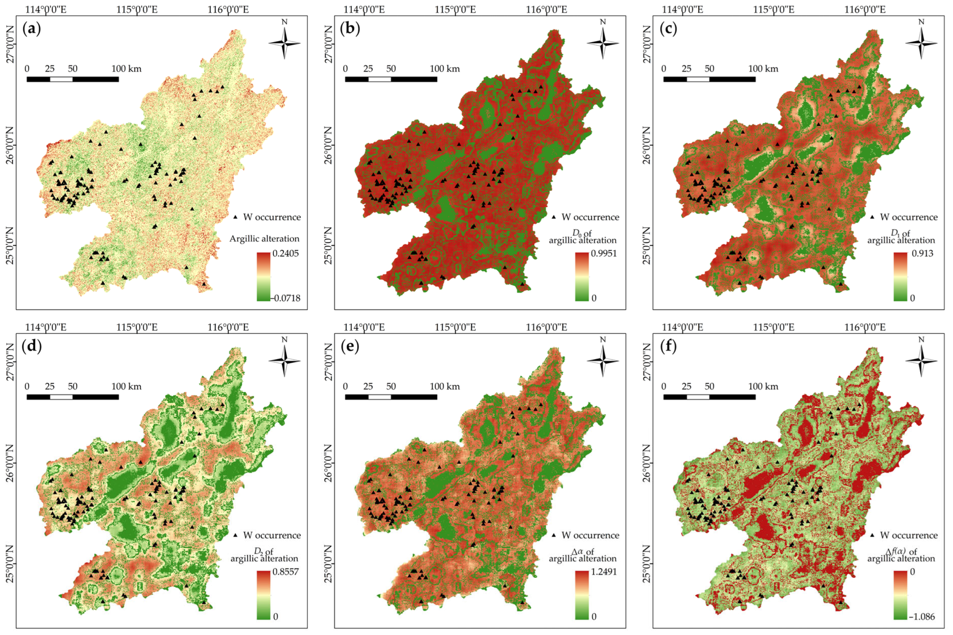
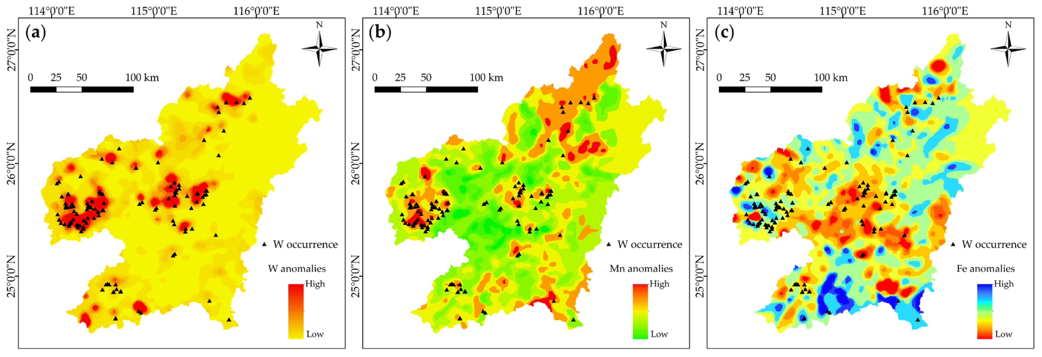
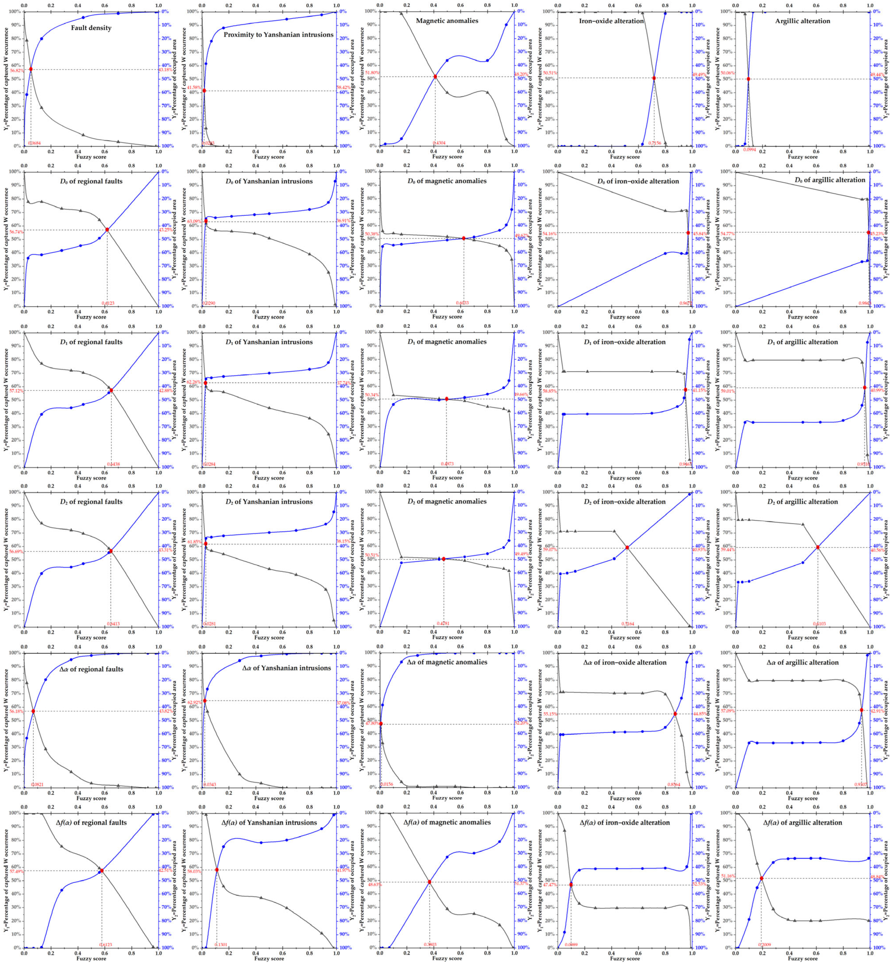
4.1. Fractal Representations of Mineralization-Related Features
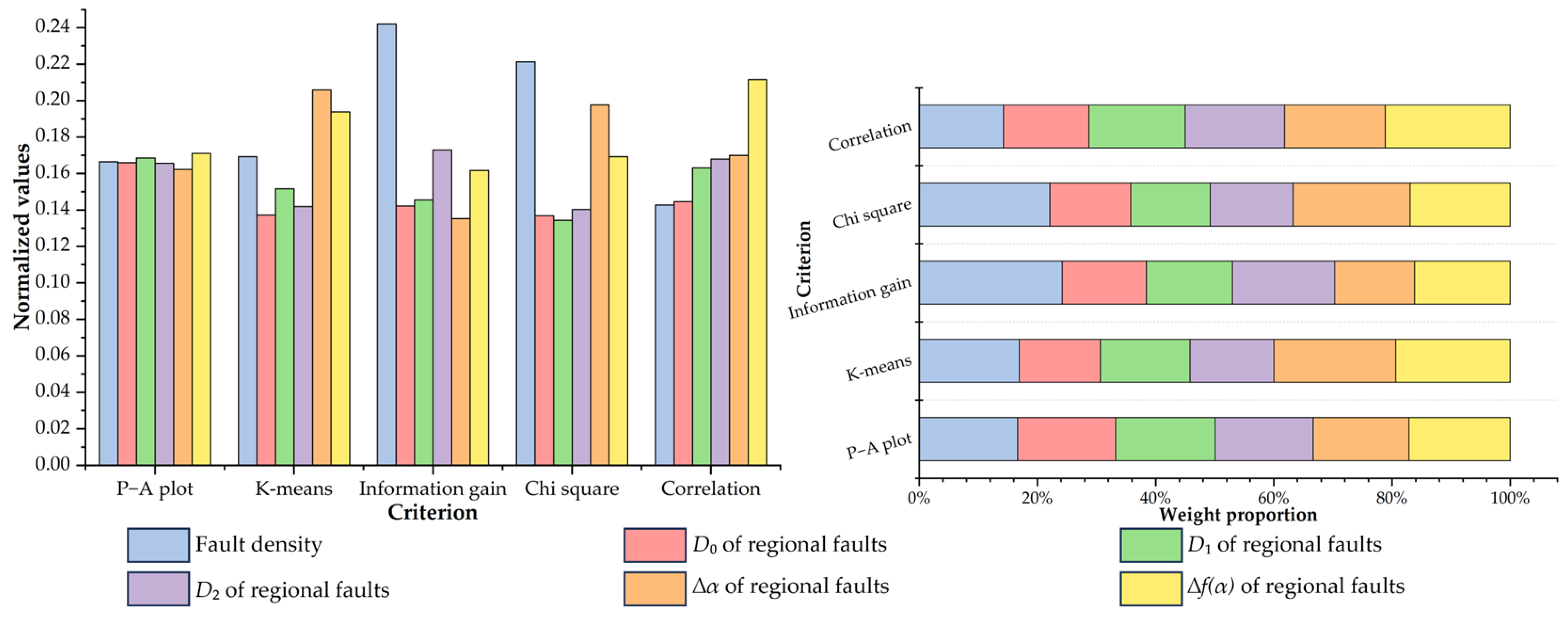
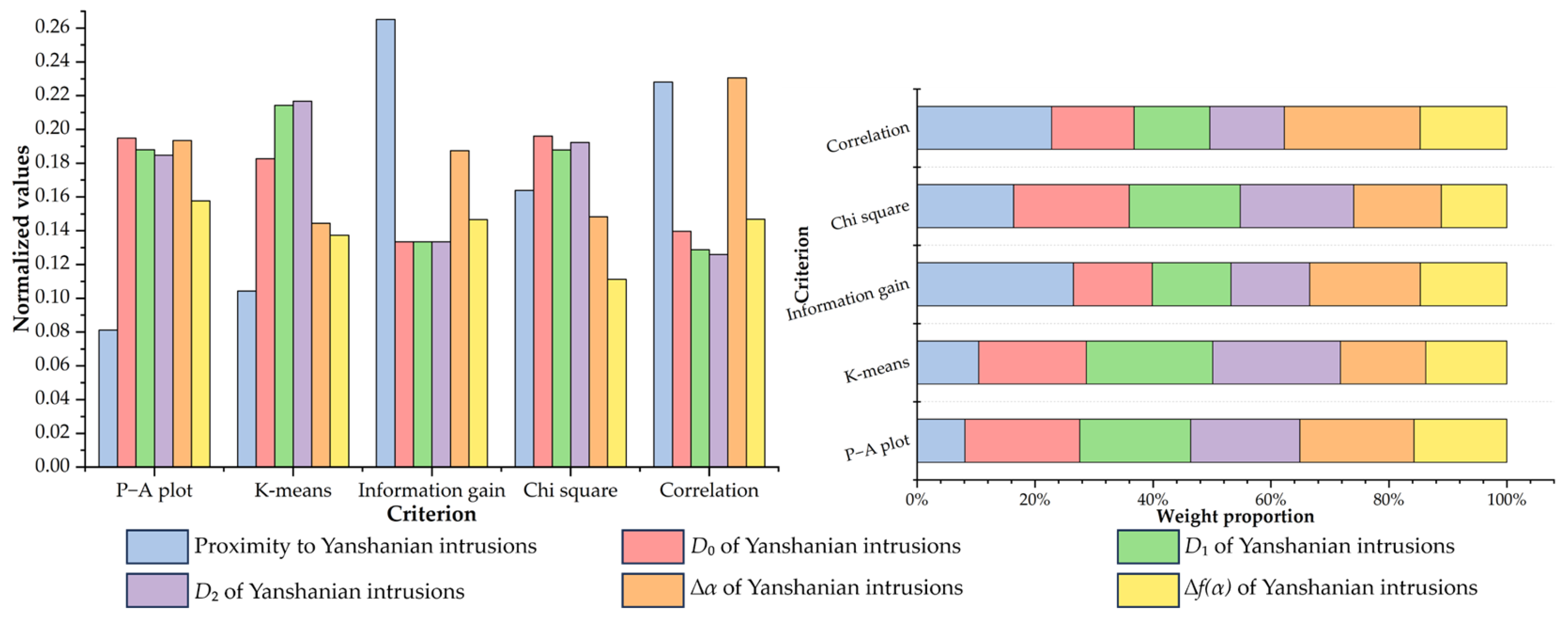
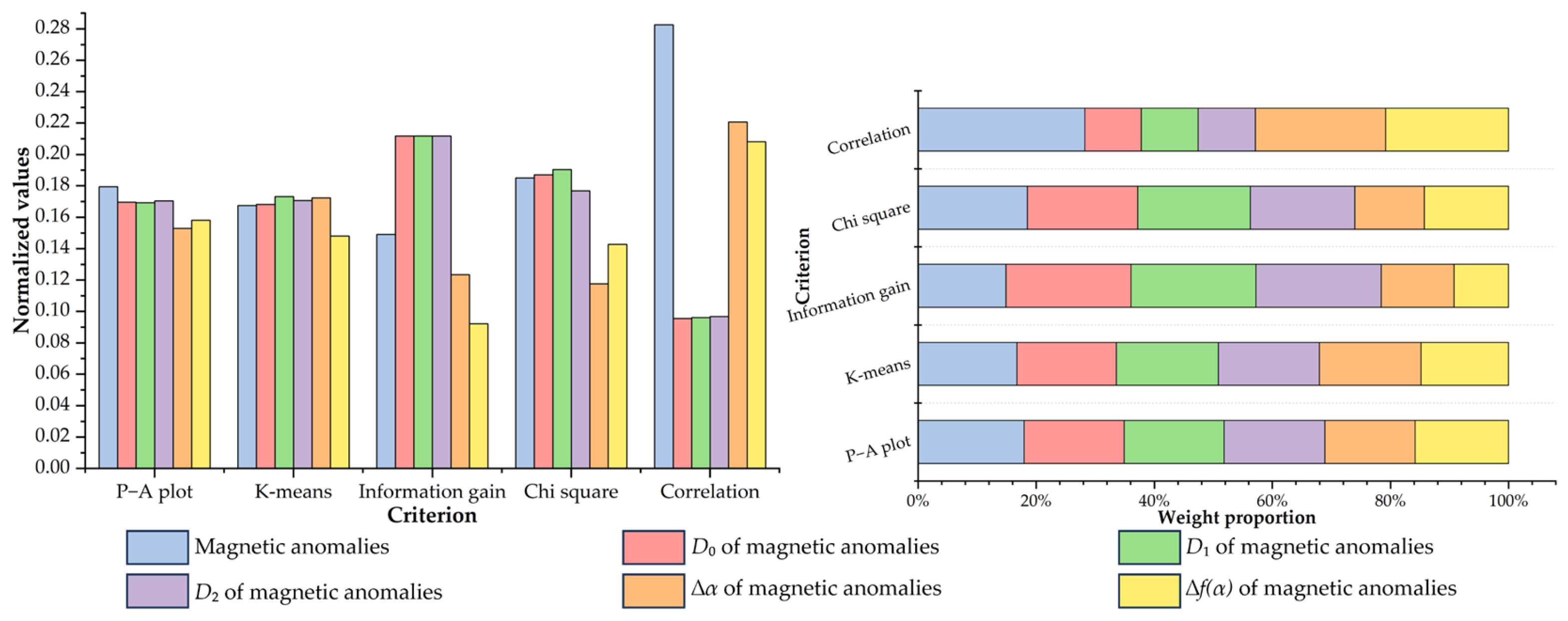
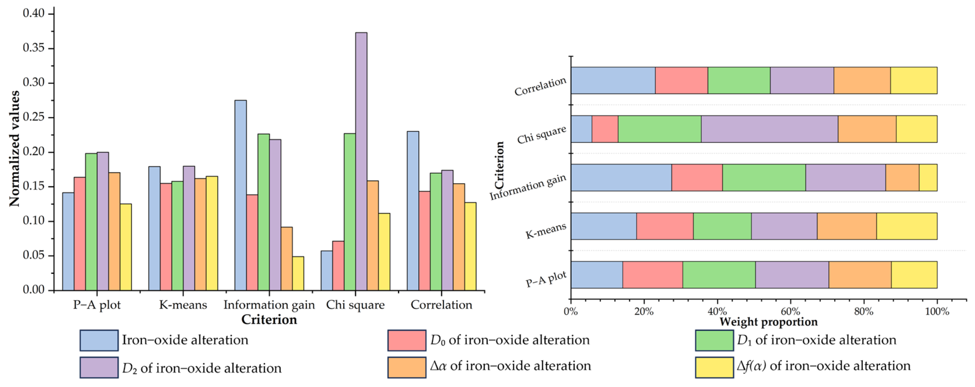
4.2. Multi-Criteria Feature Selection of Fractal Index Evidential Layers
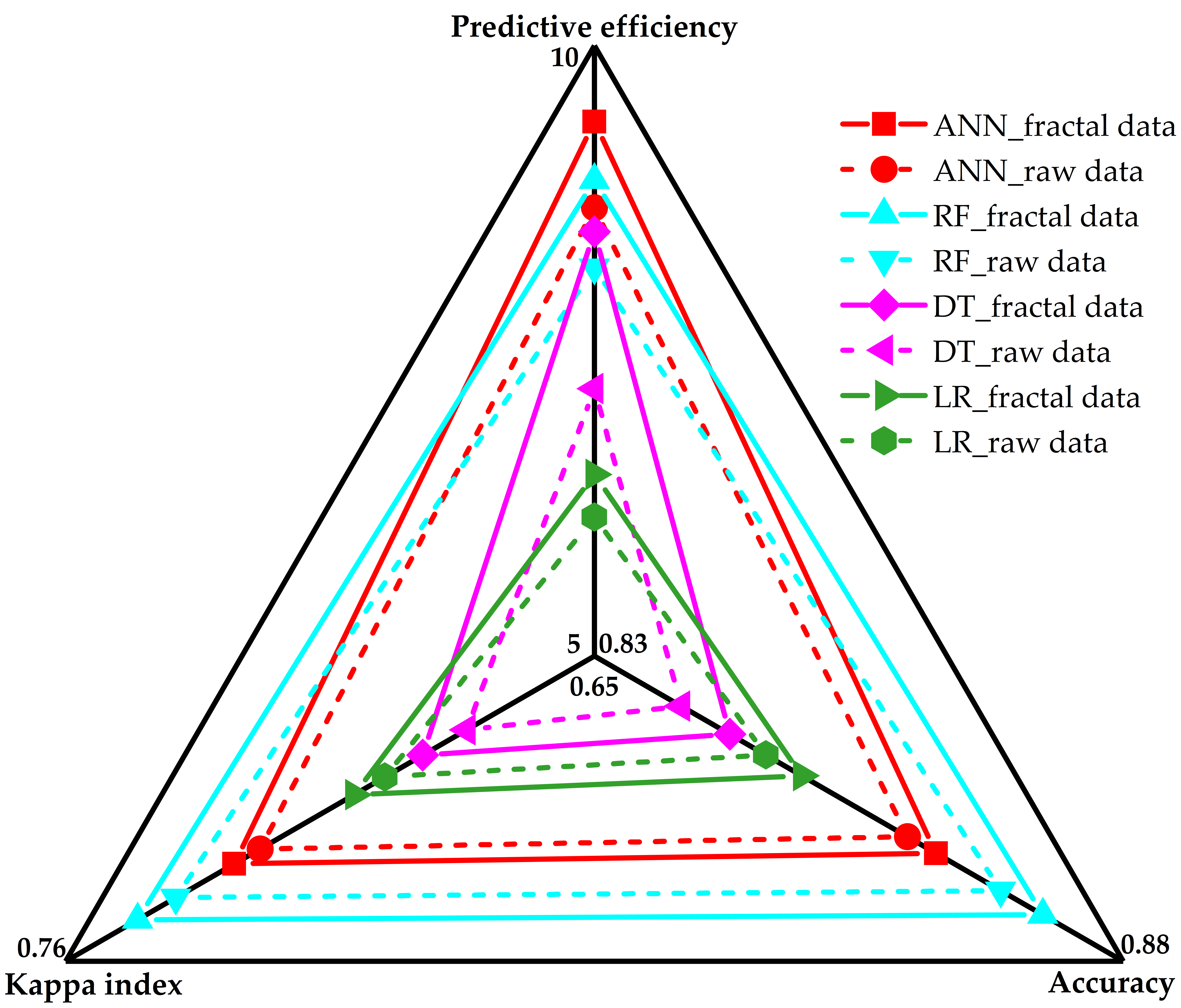
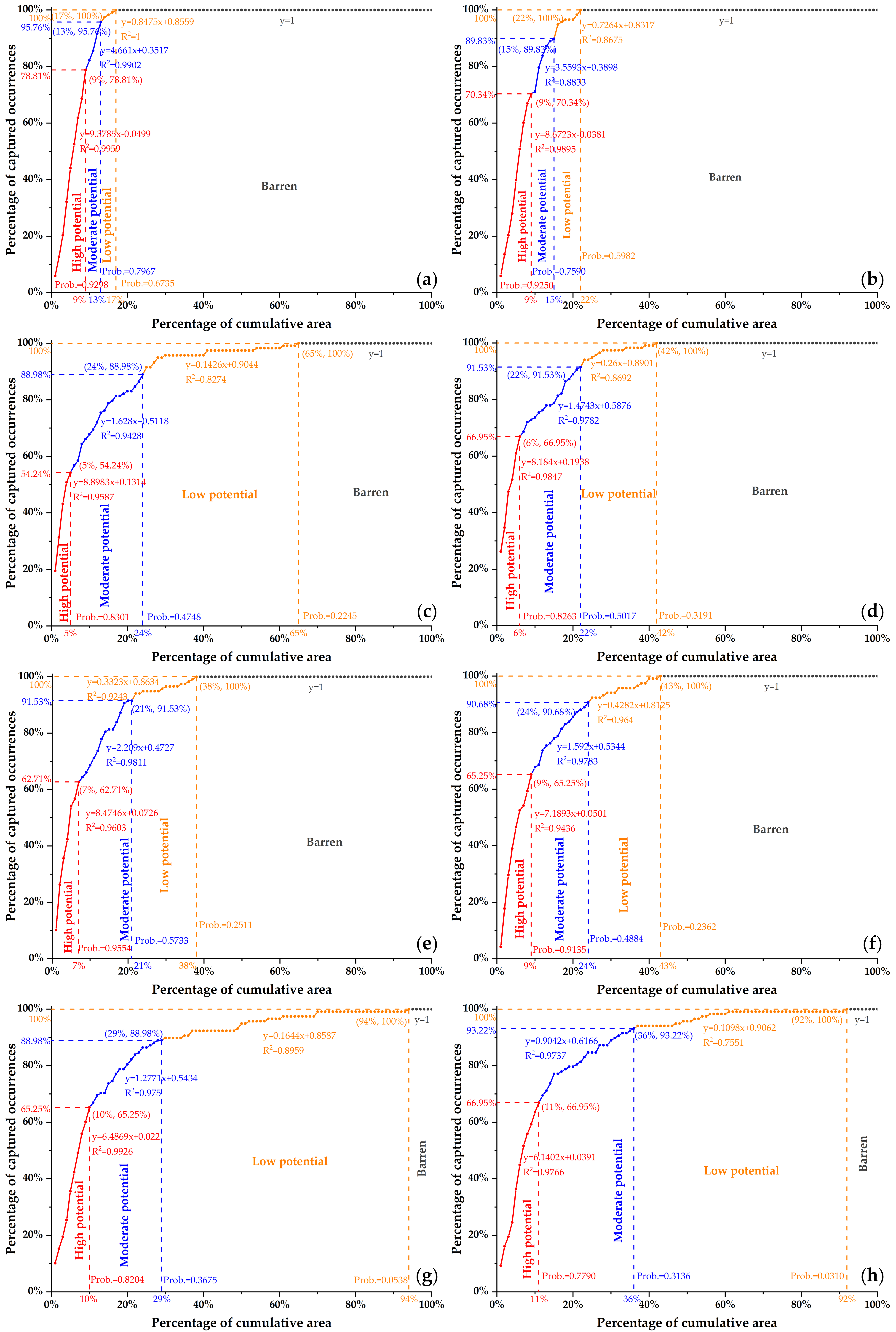
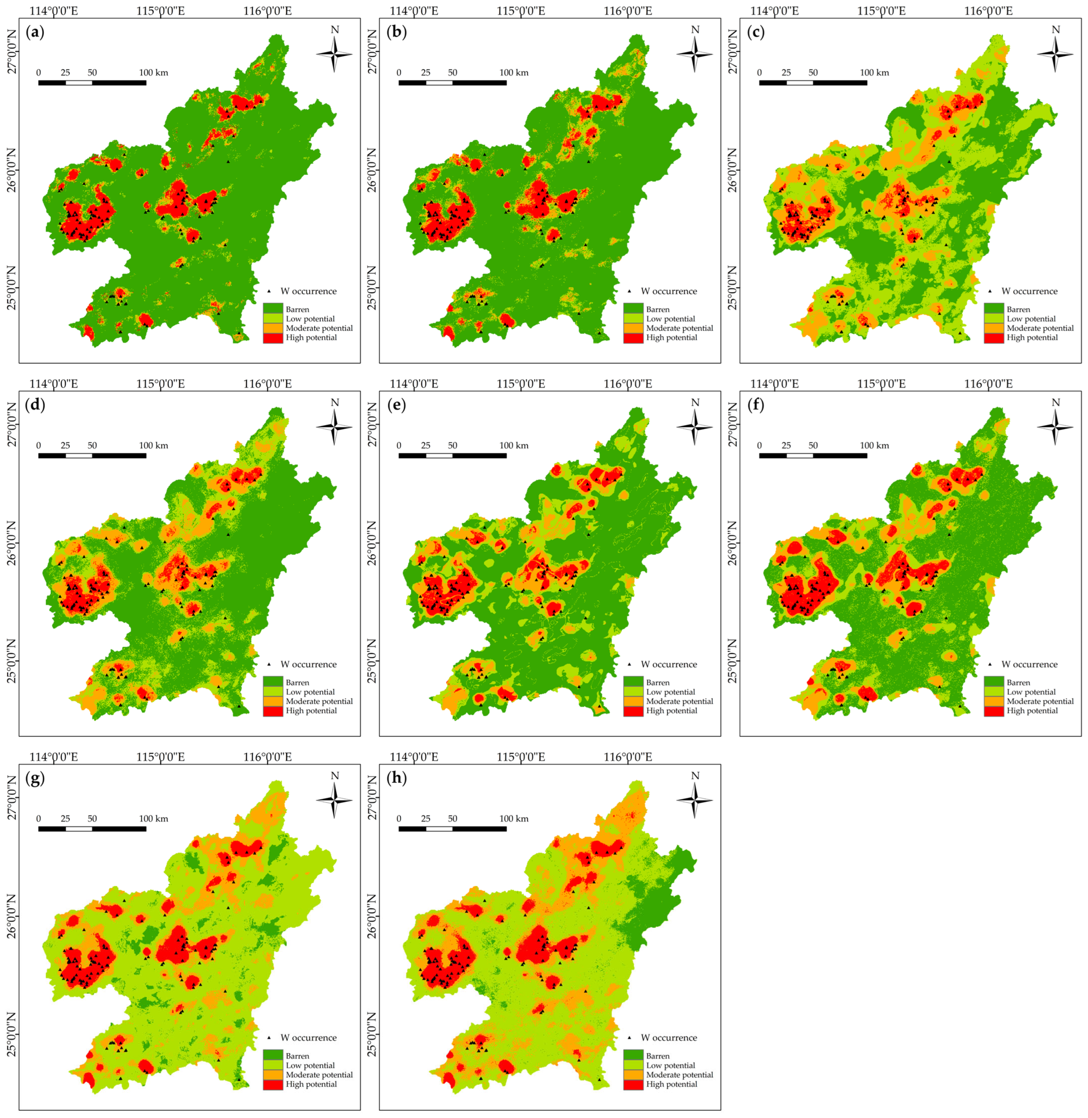
4.3. Predictive Modeling
5. Discussion
6. Conclusions
Supplementary Materials
Author Contributions
Funding
Data Availability Statement
Acknowledgments
Conflicts of Interest
References
- Zhai, M.; Hu, R.; Wang, Y.; Jiang, S.; Wang, R.; Li, J.; Chen, H.; Yang, Z.; Lü, Q.; Qi, T.; et al. Mineral Resource Science in China: Review and perspective. Geogr. Sustain. 2021, 2, 107–114. [Google Scholar] [CrossRef]
- Okada, K. Breakthrough technologies for mineral exploration. Miner. Econ. 2022, 35, 429–454. [Google Scholar] [CrossRef]
- Carranza, E.J.M. Developments in GIS-based mineral prospectivity mapping: An overview. In Proceedings of the Conference of Mineral Prospectivity, Orleans, France, 24–26 October 2017. [Google Scholar]
- Lou, Y.; Liu, Y. Mineral Prospectivity Mapping of Tungsten Polymetallic Deposits Using Machine Learning Algorithms and Comparison of Their Performance in the Gannan Region, China. Earth Space Sci. 2023, 10, e2022EA002596. [Google Scholar] [CrossRef]
- Yousefi, M.; Carranza, E.J.M.; Kreuzer, O.P.; Nykänen, V.; Hronsky, J.M.A.; Mihalasky, M.J. Data analysis methods for prospectivity modelling as applied to mineral exploration targeting: State-of-the-art and outlook. J. Geochem. Explor. 2021, 229, 106839. [Google Scholar] [CrossRef]
- Yousefi, M.; Kreuzer, O.P.; Nykänen, V.; Hronsky, J.M.A. Exploration information systems—A proposal for the future use of GIS in mineral exploration targeting. Ore Geol. Rev. 2019, 111, 103005. [Google Scholar] [CrossRef]
- Hu, X.; Li, X.; Yuan, F.; Jowitt, S.M.; Ord, A.; Ye, R.; Li, Y.; Dai, W.; Li, X.; Durance, P. 3D Numerical Simulation-Based Targeting of Skarn Type Mineralization within the Xuancheng-Magushan Orefield, Middle-Lower Yangtze Metallogenic Belt, China. Lithosphere 2020, 2020, 8351536. [Google Scholar] [CrossRef]
- Qin, Y.; Liu, L. Quantitative 3D Association of Geological Factors and Geophysical Fields with Mineralization and Its Significance for Ore Prediction: An Example from Anqing Orefield, China. Minerals 2018, 8, 300. [Google Scholar] [CrossRef]
- Zuo, R.; Carranza, E.J.M. Machine Learning-Based Mapping for Mineral Exploration. Math. Geosci. 2023, 55, 891–895. [Google Scholar] [CrossRef]
- Tessema, A. Mineral Systems Analysis and Artificial Neural Network Modeling of Chromite Prospectivity in the Western Limb of the Bushveld Complex, South Africa. Nat. Resour. Res. 2017, 26, 465–488. [Google Scholar] [CrossRef]
- Maepa, F.; Smith, R.S.; Tessema, A. Support vector machine and artificial neural network modelling of orogenic gold prospectivity mapping in the Swayze greenstone belt, Ontario, Canada. Ore Geol. Rev. 2021, 130, 103968. [Google Scholar] [CrossRef]
- Rodriguez-Galiano, V.; Sanchez-Castillo, M.; Chica-Olmo, M.; Chica-Rivas, M. Machine learning predictive models for mineral prospectivity: An evaluation of neural networks, random forest, regression trees and support vector machines. Ore Geol. Rev. 2015, 71, 804–818. [Google Scholar] [CrossRef]
- Qin, Y.; Liu, L.; Wu, W. Machine Learning-Based 3D Modeling of Mineral Prospectivity Mapping in the Anqing Orefield, Eastern China. Nat. Resour. Res. 2021, 30, 3099–3120. [Google Scholar] [CrossRef]
- Li, T.; Xia, Q.; Zhao, M.; Gui, Z.; Leng, S. Prospectivity Mapping for Tungsten Polymetallic Mineral Resources, Nanling Metallogenic Belt, South China: Use of Random Forest Algorithm from a Perspective of Data Imbalance. Nat. Resour. Res. 2019, 29, 203–227. [Google Scholar] [CrossRef]
- Xiao, F.; Chen, W.; Wang, J.; Erten, O. A Hybrid Logistic Regression: Gene Expression Programming Model and Its Application to Mineral Prospectivity Mapping. Nat. Resour. Res. 2021, 31, 2041–2064. [Google Scholar] [CrossRef]
- Li, X.; Yuan, F.; Zhang, M.; Jia, C.; Jowitt, S.M.; Ord, A.; Zheng, T.; Hu, X.; Li, Y. Three-dimensional mineral prospectivity modeling for targeting of concealed mineralization within the Zhonggu iron orefield, Ningwu Basin, China. Ore Geol. Rev. 2015, 71, 633–654. [Google Scholar] [CrossRef]
- Zuo, R.; Xiong, Y.; Wang, J.; Carranza, E.J.M. Deep learning and its application in geochemical mapping. Earth-Sci. Rev. 2019, 192, 1–14. [Google Scholar] [CrossRef]
- Sun, T.; Li, H.; Wu, K.; Chen, F.; Zhu, Z.; Hu, Z. Data-driven predictive modelling of mineral prospectivity using machine learning and deep learning methods: A case study from southern Jiangxi Province, China. Minerals 2020, 10, 102. [Google Scholar] [CrossRef]
- Xiong, Y.; Zuo, R.; Carranza, E.J.M. Mapping mineral prospectivity through big data analytics and a deep learning algorithm. Ore Geol. Rev. 2018, 102, 811–817. [Google Scholar] [CrossRef]
- Roshanravan, B.; Kreuzer, O.P.; Bruce, M.; Davis, J.; Briggs, M. Modelling gold potential in the Granites-Tanami Orogen, NT, Australia: A comparative study using continuous and data-driven techniques. Ore Geol. Rev. 2020, 125, 103661. [Google Scholar] [CrossRef]
- Hu, X.; Chen, Y.; Liu, G.; Yang, H.; Luo, J.; Ren, K.; Yang, Y. Numerical modeling of formation of the Maoping Pb-Zn deposit within the Sichuan-Yunnan-Guizhou Metallogenic Province, Southwestern China: Implications for the spatial distribution of concealed Pb mineralization and its controlling factors. Ore Geol. Rev. 2022, 140, 104573. [Google Scholar] [CrossRef]
- Hu, X.; Liu, G.; Chen, Y.; Deng, Y.; Luo, J.; Wang, K.; Yang, Y.; Li, Y. Numerical simulation of ore formation within skarn-type Pb-Zn deposits: Implications for mineral exploration and the duration of ore-forming processes. Ore Geol. Rev. 2023, 163, 105768. [Google Scholar] [CrossRef]
- Thiergärtner, H. Theory and practice in mathematical geology—Introduction and discussion. Math. Geol. 2006, 38, 659–665. [Google Scholar] [CrossRef]
- Porwal, A.; Carranza, E.J.M.; Hale, M. Artificial neural networks for mineral-potential mapping: A case study from Aravalli Province, Western India. Nat. Resour. Res. 2003, 12, 155–171. [Google Scholar] [CrossRef]
- Forouzan, M.; Arfania, R. Integration of the bands of ASTER, OLI, MSI remote sensing sensors for detection of hydrothermal alterations in southwestern area of the Ardestan, Isfahan Province, Central Iran. Egypt. J. Remote Sens. Space Sci. 2020, 23, 145–157. [Google Scholar] [CrossRef]
- Cheng, Q. Fractal Derivatives and Singularity Analysis of Frequency—Depth Clusters of Earthquakes along Converging Plate Boundaries. Fractal Fract. 2023, 7, 721. [Google Scholar] [CrossRef]
- Liu, Y.; Sun, T.; Wu, K.; Zhang, H.; Zhang, J.; Jiang, X.; Lin, Q.; Feng, M. Fractal-Based Pattern Quantification of Mineral Grains: A Case Study of Yichun Rare-Metal Granite. Fractal Fract. 2024, 8, 49. [Google Scholar] [CrossRef]
- Evertsz, C.J.; Mandelbrot, B.B. Multifractal measures. Chaos Fract. 1992, 473, 921–953. [Google Scholar]
- Zhang, Y.; He, G.; Xiao, F.; Yang, Y.; Wang, F.; Liu, Y. Geochemical Characteristics of Deep-Sea Sediments in Different Pacific Ocean Regions: Insights from Fractal Modeling. Fractal Fract. 2024, 8, 45. [Google Scholar] [CrossRef]
- Wang, W.; Pei, Y.; Cheng, Q.; Wang, W. Local Singularity Spectrum: An Innovative Graphical Approach for Analyzing Detrital Zircon Geochronology Data in Provenance Analysis. Fractal Fract. 2024, 8, 64. [Google Scholar] [CrossRef]
- Yousefi, M.; Carranza, E.J.M. Prediction–area (P–A) plot and C–A fractal analysis to classify and evaluate evidential maps for mineral prospectivity modeling. Comput. Geosci. 2015, 79, 69–81. [Google Scholar] [CrossRef]
- Wang, G.; Carranza, E.J.M.; Zuo, R.; Hao, Y.; Du, Y.; Pang, Z.; Sun, Y.; Qu, J. Mapping of district-scale potential targets using fractal models. J. Geochem. Explor. 2012, 122, 34–46. [Google Scholar] [CrossRef]
- Sun, T.; Wu, K.; Chen, L.; Liu, W.; Wang, Y.; Zhang, C. Joint Application of Fractal Analysis and Weights-of-Evidence Method for Revealing the Geological Controls on Regional-Scale Tungsten Mineralization in Southern Jiangxi Province, China. Minerals 2017, 7, 243. [Google Scholar] [CrossRef]
- Li, T.; Xia, Q.; Chang, L.; Wang, X.; Liu, Z.; Wang, S. Deposit density of tungsten polymetallic deposits in the eastern Nanling metallogenic belt, China. Ore Geol. Rev. 2018, 94, 73–92. [Google Scholar] [CrossRef]
- Cheng, Q.; Agterberg, F.P.; Ballantyne, S.B. The separation of geochemical anomalies from background by fractal methods. J. Geochem. Explor. 1994, 51, 109–130. [Google Scholar] [CrossRef]
- Zuo, R. Machine Learning of Mineralization-Related Geochemical Anomalies: A Review of Potential Methods. Nat. Resour. Res. 2017, 26, 457–464. [Google Scholar] [CrossRef]
- Ouchchen, M.; Boutaleb, S.; Abia, E.H.; El Azzab, D.; Miftah, A.; Dadi, B.; Echogdali, F.Z.; Mamouch, Y.; Pradhan, B.; Santosh, M.; et al. Exploration targeting of copper deposits using staged factor analysis, geochemical mineralization prospectivity index, and fractal model (Western Anti-Atlas, Morocco). Ore Geol. Rev. 2022, 143, 104762. [Google Scholar] [CrossRef]
- Akbari, S.; Ramazi, H.; Ghezelbash, R. Using fractal and multifractal methods to reveal geophysical anomalies in Sardouyeh District, Kerman, Iran. Earth Sci. Inform. 2023, 16, 2125–2142. [Google Scholar] [CrossRef]
- Ramezanali, A.A.; Mansouri, E.; Feizi, F. Integration of aeromagnetic geophysical data with other exploration data layers based on fuzzy AHP and C-A fractal model for Cu-porphyry potential mapping: A case study in the Fordo area, central Iran. Boll. Boll. Geofis. Teor. Appl. 2017, 58, 55–73. [Google Scholar]
- Ghezelbash, R.; Maghsoudi, A.; Carranza, E.J.M. Mapping of single- and multi-element geochemical indicators based on catchment basin analysis: Application of fractal method and unsupervised clustering models. J. Geochem. Explor. 2019, 199, 90–104. [Google Scholar] [CrossRef]
- Asl, R.A.; Afzal, P.; Adib, A.; Yasrebi, A.B. Application of multifractal modeling for the identification of alteration zones and major faults based on ETM+ multispectral data. Arab. J. Geosci. 2014, 8, 2997–3006. [Google Scholar] [CrossRef]
- Xue, B.; Zhang, M.; Browne, W.N.; Yao, X. A Survey on Evolutionary Computation Approaches to Feature Selection. IEEE Trans. Evol. Comput. 2016, 20, 606–626. [Google Scholar] [CrossRef]
- Forson, E.D.; Menyeh, A.; Wemegah, D.D.; Danuor, S.K.; Adjovu, I.; Appiah, I. Mesothermal gold prospectivity mapping of the southern Kibi-Winneba belt of Ghana based on Fuzzy analytical hierarchy process, concentration-area (C-A) fractal model and prediction-area (P-A) plot. J. Appl. Geophys. 2020, 174, 103971. [Google Scholar] [CrossRef]
- Behera, S.; Panigrahi, M.K.; Pradhan, A. Identification of geochemical anomaly and gold potential mapping in the Sonakhan Greenstone belt, Central India: An integrated concentration-area fractal and fuzzy AHP approach. Appl. Geochem. 2019, 107, 45–57. [Google Scholar] [CrossRef]
- Bai, H.; Cao, Y.; Zhang, H.; Zhang, C.; Hou, S.; Wang, W. Combining fuzzy analytic hierarchy process with concentration–area fractal for mineral prospectivity mapping: A case study involving Qinling orogenic belt in central China. Appl. Geochem. 2021, 126, 104894. [Google Scholar] [CrossRef]
- Ghaeminejad, H.; Abedi, M.; Afzal, P.; Zaynali, F.; Yousefi, M. A fractal-based outranking approach for integrating geochemical, geological, and geophysical data. Boll. Geofis. Teor. Appl. 2020, 61, 555–588. [Google Scholar]
- Zuo, R.; Wang, J. Fractal/multifractal modeling of geochemical data: A review. J. Geochem. Explor. 2016, 164, 33–41. [Google Scholar] [CrossRef]
- Behera, S.; Panigrahi, M.K. Mineral prospectivity modelling using singularity mapping and multifractal analysis of stream sediment geochemical data from the auriferous Hutti-Maski schist belt, S. India. Ore Geol. Rev. 2021, 131, 104029. [Google Scholar] [CrossRef]
- Li, X.; Yuan, F.; Zhou, T.; Deng, Y.; Zhang, D.Y.; Xu, C.; Zhang, R. Extraction of Multi-Fractal Geochemical Anomalies and Ore Genesis Prediction in the Tarbahatai-Sawuer Region, Xinjiang. Acta Petrol. Sin. 2015, 31, 426–434, (In Chinese with English abstract). [Google Scholar]
- Li, J.; Cheng, K.; Wang, S.; Morstatter, F.; Trevino, R.P.; Tang, J.; Liu, H. Feature Selection: A Data Perspective. ACM Comput. Surv. 2017, 50, 1–45. [Google Scholar] [CrossRef]
- Wang, C.; Pan, Y.; Chen, J.; Ouyang, Y.; Rao, J.; Jiang, Q. Indicator element selection and geochemical anomaly mapping using recursive feature elimination and random forest methods in the Jingdezhen region of Jiangxi Province, South China. Appl. Geochem. 2020, 122, 104760. [Google Scholar] [CrossRef]
- Zekri, H.; Cohen, D.R.; Mokhtari, A.R.; Esmaeili, A. Geochemical Prospectivity Mapping Through a Feature Extraction–Selection Classification Scheme. Nat. Resour. Res. 2018, 28, 849–865. [Google Scholar] [CrossRef]
- Forson, E.D.; Wemegah, D.D.; Hagan, G.B.; Appiah, D.; Addo-Wuver, F.; Adjovu, I.; Otchere, F.O.; Mateso, S.; Menyeh, A.; Amponsah, T. Data-driven multi-index overlay gold prospectivity mapping using geophysical and remote sensing datasets. J. Afr. Earth Sci. 2022, 190, 104504. [Google Scholar] [CrossRef]
- Riahi, S.; Bahroudi, A.; Abedi, M.; Aslani, S. Hybrid outranking of geospatial data: Multi attributive ideal-real comparative analysis and combined compromise solution. Geochemistry 2022, 82, 125898. [Google Scholar] [CrossRef]
- Yousefi, M.; Nykänen, V. Data-driven logistic-based weighting of geochemical and geological evidence layers in mineral prospectivity mapping. J. Geochem. Explor. 2016, 164, 94–106. [Google Scholar] [CrossRef]
- Feng, C.; Zeng, Z.; Zhang, D.; Qu, W.; Du, A.; Li, D.; She, H. Shrimp zircon U–Pb and molybdenite Re–Os isotopic dating of the tungsten deposits in the Tianmenshan-Hongtaoling W–Sn orefield, southern Jiangxi Province, China, and geological implications. Ore Geol. Rev. 2011, 43, 8–25. [Google Scholar] [CrossRef]
- Fang, G.; Chen, Z.; Chen, Y.; Li, J.; Zhao, B.; Zhou, X.; Zeng, Z.; Zhang, Y. Geophysical investigations of the geology and structure of the Pangushan-Tieshanlong tungsten ore field, South Jiangxi, China—Evidence for site-selection of the 2000-m nanling scientific drilling project (SP-NLSD-2). J. Asian. Earth. Sci. 2015, 110, 10–18. [Google Scholar] [CrossRef]
- GeoCloud Database of China Geological Survey. Available online: http://geocloud.cgs.gov.cn (accessed on 5 February 2024).
- Mao, J.; Cheng, Y.; Chen, M.; Pirajno, F. Major types and time–space distribution of Mesozoic ore deposits in south China and their geodynamic settings. Miner. Depos. 2013, 48, 267–294. [Google Scholar]
- Feng, C.; Zhang, D.; Zeng, Z.; Wang, S. Chronology of the tungsten deposits in southern Jiangxi Province, and episodes and zonation of the regional W-Sn mineralization-evidence from high-precision zircon U-Pb, molybdenite Re-Os and muscovite Ar-Ar ages. Acta Geol. Sin. Engl. Ed. 2012, 86, 555–567. [Google Scholar]
- Jiangxi Bureau of Geology and Mineral Resources. Mineral Prospecting and Targeting of W-Sn-Pb-Zn Deposits in Southern Jiangxi Province; Jiangxi Bureau of Geology and Mineral Resources: Nanchang, China, 2002. (In Chinese) [Google Scholar]
- Xie, X.; Mu, X.; Ren, T. Geochemical mapping in China. J. Geochem. Explor. 1997, 60, 99–113. [Google Scholar]
- Chen, X.; Fu, J. Geochemical Maps of Nanling Range; China University of Geoscience Press: Wuhan, China, 2012. (In Chinese) [Google Scholar]
- Zuo, R.; Carranza, E.J.M. Support vector machine: A tool for mapping mineral prospectivity. Comput. Geosci. 2011, 37, 1967–1975. [Google Scholar] [CrossRef]
- Carranza, E.J.M. Objective selection of suitable unit cell size in data-driven modeling of mineral prospectivity. Comput. Geosci. 2009, 35, 2032–2046. [Google Scholar] [CrossRef]
- Mandelbrot, B.B. Fractals: Form, Chance and Dimension; W.H. Freeman & Company: San Francisco, CA, USA, 1977. [Google Scholar]
- Chhabra, A.B.; Meneveau, C.; Jensen, R.V.; Sreenivasan, K.R. Direct determination of the f(α) singularity spectrum and its application to fully developed turbulence. Phys. Rev. Appl. 1989, 40, 5284–5294. [Google Scholar] [CrossRef] [PubMed]
- Mandelbrot, B.B.; Frame, M. Fractals, 1st ed.; Flammarion: Paris, France, 1997. [Google Scholar]
- Takayasu, H. Fractals in the Physical Sciences; Manchester University Press: Manchester, UK, 1990. [Google Scholar]
- Peternell, M.; Kruhl, J.H. Automation of pattern recognition and fractal-geometry-based pattern quantification, exemplified by mineral-phase distribution patterns in igneous rocks. Comput. Geosci. 2009, 35, 1415–1426. [Google Scholar] [CrossRef]
- Fry, N. Random point distributions and strain measurement in rocks. Tectonophysics 1979, 60, 89–105. [Google Scholar] [CrossRef]
- Carranza, E.J.M. Controls on mineral deposit occurrence inferred from analysis of their spatial pattern and spatial association with geological features. Ore Geol. Rev. 2009, 35, 383–400. [Google Scholar] [CrossRef]
- Haddad-Martim, P.M.; Souza Filho, C.R.d.; Carranza, E.J.M. Spatial analysis of mineral deposit distribution: A review of methods and implications for structural controls on iron oxide-copper-gold mineralization in Carajás, Brazil. Ore Geol. Rev. 2017, 81, 230–244. [Google Scholar] [CrossRef]
- Vearncombe, J.; Vearncombe, S. The spatial distribution of mineralization; applications of Fry analysis. Econ. Geol. 1999, 94, 475–486. [Google Scholar] [CrossRef]
- Zuo, R.; Agterberg, F.P.; Cheng, Q.; Yao, L. Fractal characterization of the spatial distribution of geological point processes. Int. J. Appl. Earth Obs. Geoinf. 2009, 11, 394–402. [Google Scholar] [CrossRef]
- Parsa, M.; Maghsoudi, A.; Yousefi, M. Spatial analyses of exploration evidence data to model skarn-type copper prospectivity in the Varzaghan district, NW Iran. Ore Geol. Rev. 2018, 92, 97–112. [Google Scholar] [CrossRef]
- Mandelbrot, B.B.; Wheeler, J.A. The Fractal Geometry of Nature. Am. J. Phys. 1983, 51, 286–287. [Google Scholar] [CrossRef]
- Li, L.; Chang, L.; Le, S.; Huang, D. Multifractal analysis and lacunarity analysis: A promising method for the automated assessment of muskmelon (Cucumismelo, L.) epidermis netting. Comput. Electron. Agric. 2012, 88, 72–84. [Google Scholar] [CrossRef]
- Zhao, P.; Wang, Z.; Sun, Z.; Cai, J.; Wang, L. Investigation on the pore structure and multifractal characteristics of tight oil reservoirs using NMR measurements: Permian Lucaogou Formation in Jimusaer Sag, Junggar Basin. Mar. Pet. Geol. 2017, 86, 1067–1081. [Google Scholar] [CrossRef]
- Allain, C.; Cloitre, M. Characterizing the lacunarity of random and deterministic fractal sets. Phys. Rev. A 1991, 44, 3552–3558. [Google Scholar] [CrossRef] [PubMed]
- Rodrigues, E.P.; Barbosa, M.S.; Costa Lda, F. Self-referred approach to lacunarity. Phys. Rev. E. Stat. Nonlin. Soft Matter Phys. 2005, 72, 016707. [Google Scholar] [CrossRef]
- Facon, J.; Menoti, D.; de Albuquerque Araújo, A. Lacunarity as a texture measure for address block segmentation. In Proceedings of the 10th Iberoamerican Congress on Pattern Recognition, CIARP 2005, Havana, Cuba, 15–18 November 2005. [Google Scholar]
- Cheng, Q. The gliding box method for multifractal modeling. Comput. Geosci. 1999, 25, 1073–1079. [Google Scholar] [CrossRef]
- Halsey, T.C.; Jensen, M.H.; Kadanoff, L.P.; Procaccia, I.I.; Shraiman, B.I. Fractal measures and their singularities: The characterization of strange sets. Phys. Rev. A Gen. Phys. 1986, 33, 1141–1151. [Google Scholar] [CrossRef]
- Wang, Y.; Cheng, H.; Hu, Q.; Liu, L.; Jia, L.; Gao, S.; Wang, Y. Pore structure heterogeneity of Wufeng-Longmaxi shale, Sichuan Basin, China: Evidence from gas physisorption and multifractal geometries. J. Petrol. Sci. Eng. 2022, 208, 109313. [Google Scholar] [CrossRef]
- Atmanspacher, H.; Scheingraber, H.; Wiedenmann, G. Determination of f (α) for a limited random point set. Phys. Rev. Appl. 1989, 40, 3954. [Google Scholar] [CrossRef] [PubMed]
- Vázquez, E.V.; Ferreiro, J.P.; Miranda, J.G.V.; González, A.P. Multifractal Analysis of Pore Size Distributions as Affected by Simulated Rainfall. Vadose Zone J. 2008, 7, 500–511. [Google Scholar] [CrossRef]
- Ge, X.; Fan, Y.; Li, J.; Aleem Zahid, M. Pore structure characterization and classification using multifractal theory—An application in Santanghu basin of western China. J. Pet. Sci. Eng. 2015, 127, 297–304. [Google Scholar] [CrossRef]
- Bishop, C.M. Pattern Recognition and Machine Learning; Springer: New York, NY, USA, 2006. [Google Scholar]
- Yousefi, M.; Kamkar-Rouhani, A.; Carranza, E.J.M. Application of staged factor analysis and logistic function to create a fuzzy stream sediment geochemical evidence layer for mineral prospectivity mapping. Geochem. Explor. Environ. Anal. 2013, 14, 45–58. [Google Scholar] [CrossRef]
- Cheng, Q.; Agterberg, F.P. Multifractal modeling and spatial point processes. Math. Geol. 1995, 27, 831–845. [Google Scholar] [CrossRef]
- Yousefi, M.; Carranza, E.J.M. Data-Driven Index Overlay and Boolean Logic Mineral Prospectivity Modeling in Greenfields Exploration. Nat. Resour. Res. 2015, 25, 3–18. [Google Scholar] [CrossRef]
- Yousefi, M.; Carranza, E.J.M. Fuzzification of continuous-value spatial evidence for mineral prospectivity mapping. Comput. Geosci. 2015, 74, 97–109. [Google Scholar] [CrossRef]
- Mihalasky, M.J.; Bonham-Carter, G.F. Lithodiversity and its spatial association with metallic mineral sites, Great Basin of Nevada. Nat. Resour. Res. 2001, 10, 209–226. [Google Scholar] [CrossRef]
- Steinhaus, H. Sur la division des corp materiels en parties. Bull. Acad. Pol. Sci. 1956, 1, 801. [Google Scholar]
- MacQueen, J. Some Methods for Classification and Analysis of Multivariate Observations. In Proceedings of the Fifth Berkeley Symposium on Mathematics, Statistics and Probability, Berkeley, CA, USA, 27 December–7 January 1966; University of California Press: Berkeley, CA, USA, 1967. [Google Scholar]
- Lloyd, S.P. Least Squares Quantization in PCM. IEEE Trans. Inf. Theory 1982, 28, 129–137. [Google Scholar] [CrossRef]
- Jain, A.K. Data clustering: 50 years beyond K-means. Pattern Recogn. Lett. 2010, 31, 651–666. [Google Scholar] [CrossRef]
- Meilă, M. The uniqueness of a good optimum for k-means. In Proceedings of the 23rd International Conference on Machine Learning, Pittsburgh, PA, USA, 25 June 2006. [Google Scholar]
- Tien Bui, D.; Ho, T.-C.; Pradhan, B.; Pham, B.-T.; Nhu, V.-H.; Revhaug, I. GIS-based modeling of rainfall-induced landslides using data mining-based functional trees classifier with AdaBoost, Bagging, and MultiBoost ensemble frameworks. Environ. Earth Sci. 2016, 75, 1101. [Google Scholar] [CrossRef]
- Zhou, K.; Sun, T.; Liu, Y.; Feng, M.; Tang, J.; Mao, L.; Pu, W.; Huang, J. Prospectivity Mapping of Tungsten Mineralization in Southern Jiangxi Province Using Few-Shot Learning. Minerals 2023, 13, 669. [Google Scholar] [CrossRef]
- Lee Rodgers, J.; Nicewander, W.A. Thirteen ways to look at the correlation coefficient. Am. Stat. 1988, 42, 59–66. [Google Scholar] [CrossRef]
- Pearson, K. On the criterion that a given system of deviations from the probable in the case of a correlated system of variables is such that it can be reasonably supposed to have arisen from random sampling. In Breakthroughs in Statistics; Kotz, S., Johnson, N.L., Eds.; Springer: New York, NY, USA, 1992. [Google Scholar]
- Srivastava, R. Karl Pearson and “Applied” Statistics. Resonance 2023, 28, 183–189. [Google Scholar] [CrossRef]
- McCulloch, W.S.; Pitts, W.H. A logical calculus of the ideas immanent in nervous activity. Bull. Math. Biophys. 1943, 5, 115–133. [Google Scholar] [CrossRef]
- Longbotham, N.; Chaapel, C.; Bleiler, L.; Padwick, C.; Emery, W.J.; Pacifici, F. Very High Resolution Multiangle Urban Classification Analysis. IEEE Trans. Geosci. Remote Sens. 2012, 50, 1155–1170. [Google Scholar] [CrossRef]
- Zaremotlagh, S.; Hezarkhani, A. The use of decision tree induction and artificial neural networks for recognizing the geochemical distribution patterns of LREE in the Choghart deposit, Central Iran. J. Afr. Earth Sci. 2017, 128, 37–46. [Google Scholar] [CrossRef]
- Panda, L.; Tripathy, S.K. Performance prediction of gravity concentrator by using artificial neural network—A case study. Int. J. Min. Sci. Technol. 2014, 24, 461–465. [Google Scholar] [CrossRef]
- Breiman, L.; Friedman, J.H.; Olshen, R.A.; Stone, C.J. Classification and Regression Trees; Chapman and Hall: New York, NY, USA, 1993. [Google Scholar]
- Quinlan, J.R. Introduction of decision trees. Mach. Learn. 1986, 1, 81–106. [Google Scholar] [CrossRef]
- Wu, X.; Kumar, V.; Ross Quinlan, J.; Ghosh, J.; Yang, Q.; Motoda, H.; McLachlan, G.J.; Ng, A.; Liu, B.; Yu, P.S.; et al. Top 10 algorithms in data mining. Knowl. Inf. Syst. 2007, 14, 1–37. [Google Scholar] [CrossRef]
- Chen, C.; He, B.; Zeng, Z. A method for mineral prospectivity mapping integrating C4.5 decision tree, weights-of-evidence and m-branch smoothing techniques: A case study in the eastern Kunlun Mountains, China. Earth Sci. Inform. 2013, 7, 13–24. [Google Scholar] [CrossRef]
- Breiman, L. Random forests. Mach. Learn. 2001, 45, 5–32. [Google Scholar] [CrossRef]
- Liaw, A.; Wiener, M. Classification and regression by random forest. R News 2002, 2, 18–22. [Google Scholar]
- Gislason, P.O.; Benediktsson, J.A.; Sveinsson, J.R. Random forests for land cover classification. Pattern Recogn. Lett. 2006, 27, 294–300. [Google Scholar] [CrossRef]
- Chung, C.F.; Agterberg, F.P. Regression models for estimating mineral resources from geological map data. Math. Geol. 1980, 12, 473–488. [Google Scholar] [CrossRef]
- Agterberg, F.P.; Bonham-Carter, G.F. Logistic regression and weights of evidence modeling in mineral exploration. In Proceedings of the 28th International Symposium on Application of Computer in the Mineral Industry (APCOM), Golden, CO, USA, 20–22 October 1999. [Google Scholar]
- Harris, J.R.; Sanborn-Barrie, M.; Panagapko, D.A.; Skulski, T.; Parker, J.R. Gold prospectivity maps of the Red Lake greenstone belt: Application of GIS technology. Can. J. Earth Sci. 2006, 43, 865–893. [Google Scholar] [CrossRef]
- Porwal, A.; González-Álvarez, I.; Markwitz, V.; McCuaig, T.C.; Mamuse, A. Weights-of-evidence and logistic regression modeling of magmatic nickel sulfide prospectivity in the Yilgarn Craton, Western Australia. Ore Geol. Rev. 2010, 38, 184–196. [Google Scholar] [CrossRef]
- Zhao, J.; Sui, Y.; Zhang, Z.; Zhou, M. Application of Logistic Regression and Weights of Evidence Methods for Mapping Volcanic-Type Uranium Prospectivity. Minerals 2023, 13, 608. [Google Scholar] [CrossRef]
- Yilmaz, I. Landslide susceptibility mapping using frequency ratio, logistic regression, artificial neural networks and their comparison: A case study from Kat landslides (Tokat—Turkey). Comput. Geosci. 2009, 35, 1125–1138. [Google Scholar] [CrossRef]
- Landis, J.R.; Koch, G.G. The measurement of observer agreement for categorical data. Biometrics 1977, 33, 159–174. [Google Scholar] [CrossRef] [PubMed]
- Wang, K.; Zheng, X.; Wang, G.; Liu, D.; Cui, N. A Multi-Model Ensemble Approach for Gold Mineral Prospectivity Mapping: A Case Study on the Beishan Region, Western China. Minerals 2020, 10, 1126. [Google Scholar] [CrossRef]
- Fabbri, A.G.; Chung, C.J. On Blind Tests and Spatial Prediction Models. Nat. Resour. Res. 2008, 17, 107–118. [Google Scholar] [CrossRef]
- Zuo, R.; Cheng, Q.; Agterberg, F.P. Application of a hybrid method combining multilevel fuzzy comprehensive evaluation with asymmetric fuzzy relation analysis to mapping prospectivity. Ore Geol. Rev. 2009, 35, 101–108. [Google Scholar] [CrossRef]
- Rodriguez-Galiano, V.F.; Chica-Olmo, M.; Chica-Rivas, M. Predictive modelling of gold potential with the integration of multisource information based on random forest: A case study on the Rodalquilar area, Southern Spain. Int. J. Geogr. Inf. Sci. 2014, 28, 1336–1354. [Google Scholar] [CrossRef]
- Zuo, R.; Zhang, Z.; Zhang, D.; Carranza, E.J.M.; Wang, H. Evaluation of uncertainty in mineral prospectivity mapping due to missing evidence: A case study with skarn-type Fe deposits in Southwestern Fujian Province, China. Ore Geol. Rev. 2015, 71, 502–515. [Google Scholar] [CrossRef]
- Parsa, M.; Carranza, E.J.M. Modulating the Impacts of Stochastic Uncertainties Linked to Deposit Locations in Data-Driven Predictive Mapping of Mineral Prospectivity. Nat. Resour. Res. 2021, 30, 3081–3097. [Google Scholar] [CrossRef]
- Parsa, M.; Lentz, D.R.; Walker, J.A. Predictive Modeling of Prospectivity for VHMS Mineral Deposits, Northeastern Bathurst Mining Camp, NB, Canada, Using an Ensemble Regularization Technique. Nat. Resour. Res. 2022, 32, 19–36. [Google Scholar] [CrossRef]
- Lundberg, S.M.; Lee, S.I. A unified approach to interpreting model predictions. In Proceedings of the 31st International Conference on Neural Information Processing Systems, Long Beach, CA, USA, 4 December 2017. [Google Scholar]
- Marcilio, W.E.; Eler, D.M. From Explanations to Feature Selection: Assessing SHAP Values as feature Selection Mechanism. In Proceedings of the 33rd SIBGRAPI Conference on Graphics, Patterns and Images, Online, 7 November 2020. [Google Scholar]
- Luo, Z.; Zuo, R.; Xiong, Y.; Zhou, B. Metallogenic-Factor Variational Autoencoder for Geochemical Anomaly Detection by Ad-Hoc and Post-Hoc Interpretability Algorithms. Nat. Resour. Res. 2023, 32, 835–853. [Google Scholar] [CrossRef]
- Pradhan, B.; Jena, R.; Talukdar, D.; Mohanty, M.; Sahu, B.K.; Raul, A.K.; Abdul Maulud, K.N. A New Method to Evaluate Gold Mineralisation-Potential Mapping Using Deep Learning and an Explainable Artificial Intelligence (XAI) Model. Remote Sens. 2022, 14, 4486. [Google Scholar] [CrossRef]
- Carranza, E.J.M.; Hale, M.; Faassen, C. Selection of coherent deposit-type locations and their application in data-driven mineral prospectivity mapping. Ore Geol. Rev. 2008, 33, 536–558. [Google Scholar] [CrossRef]
- Sun, T.; Chen, F.; Zhong, L.; Liu, W.; Wang, Y. GIS-based mineral prospectivity mapping using machine learning methods: A case study from Tongling ore district, eastern China. Ore Geol. Rev. 2019, 109, 26–49. [Google Scholar] [CrossRef]
- Prado, E.M.G.; de Souza Filho, C.R.; Carranza, E.J.M.; Motta, J.G. Modeling of Cu-Au prospectivity in the Carajás mineral province (Brazil) through machine learning: Dealing with imbalanced training data. Ore Geol. Rev. 2020, 124, 103611. [Google Scholar] [CrossRef]
- Yang, J.; Kang, L.; Peng, J.; Zhong, H.; Gao, J.; Liu, L. In-situ elemental and isotopic compositions of apatite and zircon from the Shuikoushan and Xihuashan granitic plutons: Implication for Jurassic granitoid-related Cu-Pb-Zn and W mineralization in the Nanling Range, south China. Ore Geol. Rev. 2018, 93, 382–403. [Google Scholar] [CrossRef]
- Yang, J.; Kang, L.; Liu, L.; Peng, J.; Qi, Y. Tracing the origin of ore-forming fluids in the Piaotang tungsten deposit, south China: Constraints from in-situ analyses of wolframite and individual fluid inclusion. Ore Geol. Rev. 2019, 111, 102939. [Google Scholar] [CrossRef]
- Zhao, W.; Zhou, M.; Li, Y.; Zhao, Z.; Gao, J. Genetic types, mineralization styles, and geodynamic settings of Mesozoic tungsten deposits in south China. J. Asian Earth Sci. 2017, 137, 109–140. [Google Scholar] [CrossRef]
- Editorial Committee of China Mineral Geological Record. The Mineral Geological Records of China: Volume of Jiangxi Province; Geology Publishing House: Beijing, China, 2015. (In Chinese) [Google Scholar]


| P–A Plot | K-Means | Information Gain | Chi-Square | Correlation | Average Rank | ||||||||||
|---|---|---|---|---|---|---|---|---|---|---|---|---|---|---|---|
| Pr | Oa | Nd | Rank | Pk | Ok | Nk | Rank | Value | Rank | Value | Rank | Value | Rank | ||
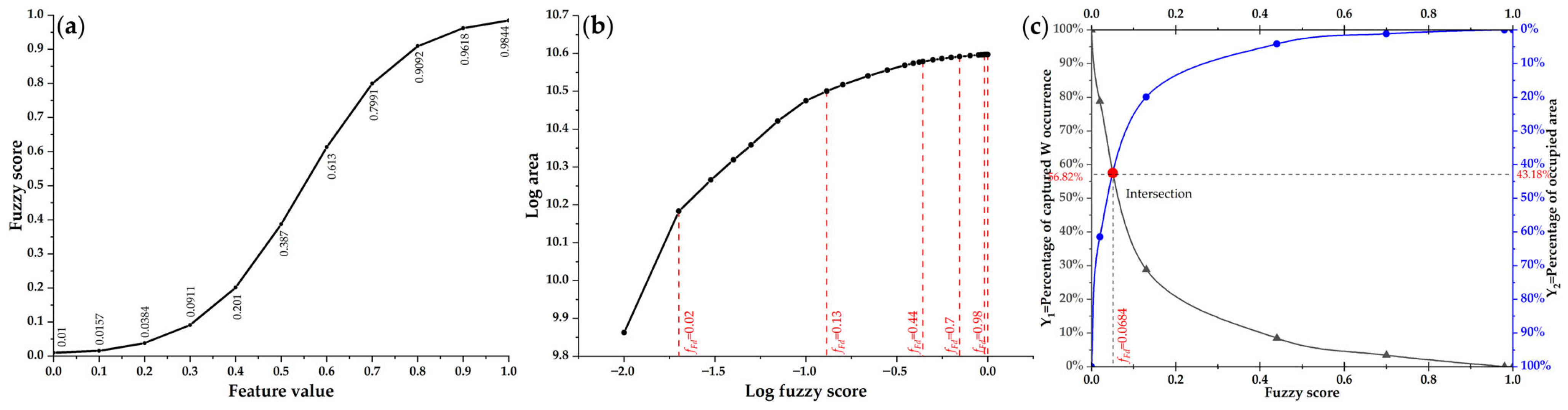
| Fauden | 56.82% | 43.18% | 1.3159 | 3 | 14.41% | 6.78% | 2.1254 | 3 | 0.2422 | 1 | 26.4954 | 1 | 0.1964 | 1 | 1.8 |
| Fauden_D0 | 56.75% | 43.25% | 1.3121 | 4 | 9.32% | 5.41% | 1.7227 | 6 | 0.1422 | 5 | 16.3944 | 5 | 0.1514 | 4 | 4.8 |
| Fauden_D1 | 57.12% | 42.88% | 1.3321 | 2 | 10.17% | 5.34% | 1.9045 | 4 | 0.1456 | 4 | 16.0892 | 6 | 0.1560 | 3 | 3.8 |
| Fauden_D2 | 56.69% | 43.31% | 1.3089 | 5 | 9.32% | 5.24% | 1.7786 | 5 | 0.1731 | 2 | 16.8138 | 4 | 0.1579 | 2 | 3.6 |
| Fauden_∆α | 56.18% | 43.82% | 1.2821 | 6 | 9.32% | 3.61% | 2.5817 | 1 | 0.1352 | 6 | 23.6836 | 2 | 0.1325 | 6 | 4.2 |
| Fauden_∆f(α) | 57.49% | 42.51% | 1.3524 | 1 | 9.32% | 3.83% | 2.4334 | 2 | 0.1617 | 3 | 20.2765 | 3 | 0.1342 | 5 | 2.8 |
| Granite | 41.58% | 58.42% | 0.7117 | 6 | 28.81% | 10.06% | 2.8638 | 6 | 0.2651 | 1 | 56.8926 | 4 | 0.2961 | 2 | 3.8 |
| Granite_D0 | 63.09% | 36.91% | 1.7093 | 1 | 10.17% | 2.03% | 5.0099 | 3 | 0.1336 | 6 | 68.0716 | 1 | 0.1814 | 4 | 3 |
| Granite_D1 | 62.26% | 37.74% | 1.6497 | 3 | 10.17% | 1.73% | 5.8786 | 2 | 0.1336 | 5 | 65.2276 | 3 | 0.1672 | 5 | 3.6 |
| Granite_D2 | 61.85% | 38.15% | 1.6212 | 4 | 10.17% | 1.71% | 5.9474 | 1 | 0.1336 | 4 | 66.7266 | 2 | 0.1635 | 6 | 3.4 |
| Granite_∆α | 62.92% | 37.08% | 1.6969 | 2 | 11.02% | 2.78% | 3.9640 | 4 | 0.1875 | 2 | 51.4997 | 5 | 0.2991 | 1 | 2.8 |
| Granite_∆f(α) | 58.03% | 41.97% | 1.3827 | 5 | 11.02% | 2.92% | 3.7740 | 5 | 0.1467 | 3 | 38.6398 | 6 | 0.1907 | 3 | 4.4 |
| Mag | 51.80% | 48.20% | 1.0747 | 1 | 34.75% | 26.54% | 1.3093 | 5 | 0.1490 | 4 | 11.9883 | 3 | 0.1022 | 1 | 2.8 |
| Mag_D0 | 50.38% | 49.62% | 1.0153 | 3 | 30.51% | 23.21% | 1.3145 | 4 | 0.2117 | 3 | 12.1122 | 2 | 0.0345 | 6 | 3.6 |
| Mag_D1 | 50.34% | 49.66% | 1.0137 | 4 | 26.27% | 19.41% | 1.3534 | 1 | 0.2117 | 2 | 12.3268 | 1 | 0.0348 | 5 | 2.6 |
| Mag_D2 | 50.51% | 49.49% | 1.0206 | 2 | 26.27% | 19.70% | 1.3335 | 3 | 0.2117 | 1 | 11.4590 | 4 | 0.0350 | 4 | 2.8 |
| Mag_∆α | 47.80% | 52.20% | 0.9157 | 6 | 9.32% | 6.92% | 1.3468 | 2 | 0.1235 | 5 | 7.6186 | 6 | 0.0798 | 2 | 4.2 |
| Mag_∆f(α) | 48.63% | 51.37% | 0.9467 | 5 | 11.02% | 9.52% | 1.1576 | 6 | 0.0923 | 6 | 9.2446 | 5 | 0.0753 | 3 | 5 |
| RSFe | 50.51% | 49.49% | 1.0206 | 5 | 11.02% | 4.23% | 2.6052 | 2 | 0.2753 | 1 | 4.9470 | 6 | 0.1635 | 1 | 3 |
| RSFe_D0 | 54.16% | 45.84% | 1.1815 | 4 | 12.71% | 5.65% | 2.2496 | 6 | 0.1387 | 4 | 6.1530 | 5 | 0.1020 | 5 | 4.8 |
| RSFe_D1 | 58.85% | 41.15% | 1.4301 | 2 | 16.95% | 7.38% | 2.2967 | 5 | 0.2267 | 2 | 19.5754 | 2 | 0.1207 | 3 | 2.8 |
| RSFe_D2 | 59.07% | 40.93% | 1.4432 | 1 | 12.71% | 4.87% | 2.6099 | 1 | 0.2185 | 3 | 32.1731 | 1 | 0.1235 | 2 | 1.6 |
| RSFe_∆α | 55.15% | 44.85% | 1.2297 | 3 | 14.41% | 6.12% | 2.3546 | 4 | 0.0918 | 5 | 13.6986 | 3 | 0.1098 | 4 | 3.8 |
| RSFe_∆f(α) | 47.47% | 52.53% | 0.9037 | 6 | 10.17% | 4.24% | 2.3986 | 3 | 0.0491 | 6 | 9.6391 | 4 | 0.0904 | 6 | 5 |
| RSOH | 50.06% | 49.94% | 1.0024 | 6 | 13.56% | 4.68% | 2.8974 | 3 | 0.1305 | 4 | 23.0229 | 3 | 0.1002 | 6 | 4.4 |
| RSOH_D0 | 54.77% | 45.23% | 1.2109 | 4 | 11.86% | 4.03% | 2.9429 | 2 | 0.1741 | 3 | 10.0611 | 6 | 0.1512 | 3 | 3.6 |
| RSOH_D1 | 59.01% | 40.99% | 1.4396 | 2 | 17.80% | 8.10% | 2.1975 | 5 | 0.2473 | 2 | 31.6592 | 2 | 0.1731 | 2 | 2.6 |
| RSOH_D2 | 59.44% | 40.56% | 1.4655 | 1 | 17.80% | 7.57% | 2.3514 | 4 | 0.2531 | 1 | 40.0043 | 1 | 0.1900 | 1 | 1.6 |
| RSOH_∆α | 57.09% | 42.91% | 1.3305 | 3 | 15.25% | 7.48% | 2.0388 | 6 | 0.1175 | 5 | 17.2985 | 5 | 0.1510 | 4 | 4.6 |
| RSOH_∆f(α) | 51.16% | 48.84% | 1.0475 | 5 | 10.17% | 3.25% | 3.1292 | 1 | 0.0774 | 6 | 21.3614 | 4 | 0.1155 | 5 | 4.2 |
| Model | W Occurrence% | Involved Cells% | Targeting Efficiency |
|---|---|---|---|
| Fractal-trained ANN | 78.81% | 8.55% | 9.2175 |
| Raw-data-trained ANN | 70.34% | 8.61% | 8.1696 |
| Fractal-trained RF | 50.85% | 4.64% | 10.9591 |
| Raw-data-trained RF | 55.93% | 5.67% | 9.8642 |
| Fractal-trained DT | 62.71% | 7.45% | 8.4174 |
| Raw-data-trained DT | 63.56% | 8.64% | 7.3565 |
| Fractal-trained LR | 65.25% | 9.83% | 6.6378 |
| Raw-data-trained LR | 66.95% | 10.51% | 6.3701 |
Disclaimer/Publisher’s Note: The statements, opinions and data contained in all publications are solely those of the individual author(s) and contributor(s) and not of MDPI and/or the editor(s). MDPI and/or the editor(s) disclaim responsibility for any injury to people or property resulting from any ideas, methods, instructions or products referred to in the content. |
© 2024 by the authors. Licensee MDPI, Basel, Switzerland. This article is an open access article distributed under the terms and conditions of the Creative Commons Attribution (CC BY) license (https://creativecommons.org/licenses/by/4.0/).
Share and Cite
Sun, T.; Feng, M.; Pu, W.; Liu, Y.; Chen, F.; Zhang, H.; Huang, J.; Mao, L.; Wang, Z. Fractal-Based Multi-Criteria Feature Selection to Enhance Predictive Capability of AI-Driven Mineral Prospectivity Mapping. Fractal Fract. 2024, 8, 224. https://doi.org/10.3390/fractalfract8040224
Sun T, Feng M, Pu W, Liu Y, Chen F, Zhang H, Huang J, Mao L, Wang Z. Fractal-Based Multi-Criteria Feature Selection to Enhance Predictive Capability of AI-Driven Mineral Prospectivity Mapping. Fractal and Fractional. 2024; 8(4):224. https://doi.org/10.3390/fractalfract8040224
Chicago/Turabian StyleSun, Tao, Mei Feng, Wenbin Pu, Yue Liu, Fei Chen, Hongwei Zhang, Junqi Huang, Luting Mao, and Zhiqiang Wang. 2024. "Fractal-Based Multi-Criteria Feature Selection to Enhance Predictive Capability of AI-Driven Mineral Prospectivity Mapping" Fractal and Fractional 8, no. 4: 224. https://doi.org/10.3390/fractalfract8040224
APA StyleSun, T., Feng, M., Pu, W., Liu, Y., Chen, F., Zhang, H., Huang, J., Mao, L., & Wang, Z. (2024). Fractal-Based Multi-Criteria Feature Selection to Enhance Predictive Capability of AI-Driven Mineral Prospectivity Mapping. Fractal and Fractional, 8(4), 224. https://doi.org/10.3390/fractalfract8040224