Analytical Scheme for Time Fractional Kawahara and Modified Kawahara Problems in Shallow Water Waves

Abstract

The Kawahara equation exhibits signal dispersion across lines of transmission and the production of unstable waves from the water in the broad wavelength area. This article explores the computational analysis for the approximate series of time fractional Kawahara (TFK) and modified Kawahara (TFMK) problems. We utilize the Shehu homotopy transform method (SHTM), which combines the Shehu transform (ST) with the homotopy perturbation method (HPM). He’s polynomials using HPM effectively handle the nonlinear terms. The derivatives of fractional order are examined in the Caputo sense. The suggested methodology remains unaffected by any assumptions, restrictions, or hypotheses on variables that could potentially pervert the fractional problem. We present numerical findings via visual representations to indicate the usability and performance of fractional order derivatives for depicting water waves in long-wavelength regions. The significance of our proposed scheme is demonstrated by the consistency of analytical results that align with the exact solutions. These derived results demonstrate that SHTM is an effective and powerful scheme for examining the results in the representation of series for time-fractional problems.

1. Introduction

Fractional differential equations (FDEs) have been utilized in numerous domains consisting of computational biological sciences, physical sciences, quantum science, astrophysics, solid-state physics, hydrodynamics, plasma physics, and optic fibers [1,2,3,4]. The importance of fractional calculus in applied mathematics has expanded significantly, and as a result, these FDEs have become highly appealing for modeling real-life occurrences in nature. Numerous scientists from diverse disciplines have demonstrated that solving these equations is a valuable and intriguing field of study [5,6]. Numerous scholars have recently discovered valuable strategies for dealing with these types of models in the disciplines of mathematical science and engineering, including Iterative transform scheme [7], Laplace residual power series approach [8], finite difference scheme [9], generalized Kudryashov approach [10], sub-equation strategy [11], generalized Riccati equation method [12], exponential rational function method [13], tanh method [14], and many other techniques [15,16].

The study of nonlinear equations for traveling wave solutions has significantly enhanced in nonlinear physical systems. Many branches of science and engineering have investigated nonlinear wave dynamics. These include geological sciences, hydrodynamics, solid-state physics, fiber optics, and plasma physics. The Kawahara equation is important in numerous areas of physical sciences and ocean technology. The TFK problem enhances this process by integrating memory effects, resulting in more precise formulations of waves propagating in complex media of temporal behaviors. Kaya and Al-Khaled [17] studied the concept of the Adomian decomposition method for the traveling wave solutions of the Kawahara equation. Daşcıoğluand Ünal [18] proposed a direct approach built on the Jacobi elliptic functions for the analytical results of the space-time fractional Kawahara problem. Başhan [19] obtained the solutions in numerical format for the Kawahara problem via the Crank–Nicolson scheme based on modified cubic B-splines. In 1972, Kawahara first proposed the Kawahara equations to depict the propagation of solitary waves in media [20]. It exists in the domain of plasma magneto-acoustic waves and surface tension in shallow water. Furthermore, TFMK incorporates an extensive variety of applications, including capillary gravitational wave propagation and plasma waves [21,22,23]. This study aims to explore an effective strategy for utilizing SHTM to derive the analytical results of TFK and TFMK problems. The equations under investigation are as follows: The TFK problems is expressed as

$$\begin{array}{c}\hfill D_t^{\alpha }u(x,t)+u(x,t)u_x(x,t)+u_{xxx}(x,t)-u_{xxxxx}(x,t)=0\end{array}$$

(1)

towards the following constraints

$$\begin{array}{c}\hfill u(x,0)=f(x)\end{array}$$

(2)

and the TFMK problem is expressed as

$$\begin{array}{c}\hfill D_t^{\alpha }u(x,t)+u^2(x,t)u_x(x,t)+a{u}_{xxx}(x,t)+b{u}_{xxxxx}(x,t)=0\end{array}$$

(3)

towards the following constraints

$$\begin{array}{c}\hfill u(x,0)=g(x)\end{array}$$

(4)

whereas $a>0$ and $b<0$ are non zero constants and $u(x,t)$ is the function of the spatial variable x and time t. $f(x)$ and $g(x)$ are defined on interval $-\infty <x<\infty$. The dispersion equations for waves play a crucial role in applied physics and mathematics. These equations offer significant value in exhibiting complex systems with memory effects. It also plays a crucial role in improving the ability to predict and contribute to advancements in applied and theoretical aspects of science and engineering, such as electromagnetic waves in plasma, surface tension vibrations in shallow seas, and gravitational waves in vessels. Recently, various researchers have obtained the analytical results of TFK and TFMK problems utilizing a broad range of schemes, including Elzaki transform decomposition method [24], natural transform decomposition method [25], and the residual power series method [26]. The authors [27,28,29] examined the estimated outcomes of these fractional differential problems and demonstrated that these problems are significantly more intricate than their integer-order counterparts when it comes to achieving precise outcomes.

This work focuses on utilizing SHTM to deal with the analytical results solutions of TFK and TFMK problems. The Shehu transform (ST) and homotopy perturbation method (HPM) are powerful techniques used to enhance the effectiveness of SHTM. The proposed method provides a more efficient procedure for calculating series terms in comparison to conventional Adomian and perturbation strategies. This method eliminates the need for computing derivatives or integrals of fractional order in the recurrence equation. Thus, this technique can be efficiently utilized for solving specific classes of nonlinear FDEs promptly. This technique offers a highly accurate approximation solution that leads to precise results using a rapid convergence series. Many physical issues, particularly fractional-order challenges have been investigated using ST and HPM, such as Caputo-type initial value problems [30], nonlinear evolution equation [31], gas dynamics equation [32], Cauchy-reaction diffusion equation [33], advection-dispersion equation [34], and nonlinear delay differential equations [35].

This paper is organized in a specific manner: Section 2 presents an overview of fractional calculus and the Shehu transform. The scientific development of SHTM is described in Section 3. Section 4 covers existences and uniqueness with convergence analysis. In Section 5, we address two numerical problems involving time-fractional order and present their approximate results obtained through the use of SHTM. The results and discussion are provided in Section 6. The closing remarks of the conclusion are presented in Section 7.

2. Preliminaries

In this part, we outline some properties and ideas of $\mathcal{A}$IT that are crucial to the development of this framework.

Definition 1.

The order of the Riemann–Liouville (R-L) operator is expressed as [24,26]

$$\begin{array}{c}\hfill D^{\alpha }u(t)=\left\{\begin{array}{c}{\displaystyle \frac{d^{\phi }}{d{t}^{\phi }}}u(t),\alpha =\phi ,\hfill \\ {\displaystyle \frac{1}{\Gamma (\phi -\alpha )}}{\displaystyle \frac{d}{d{t}^{\phi }}}{\int }_0^{t}u(t){(t-\varphi )}^{\phi -\alpha -1}d\varphi ,\phi -1<\alpha <\phi ,\hfill \end{array}\right.\end{array}$$

where $\phi \in Z^{+},\alpha \in R^{+}$ and

$$\begin{array}{c}\hfill D^{-\alpha }u(t)=\frac{1}{\Gamma (\alpha )}{\int }_0^t{\left(t-{\varphi }^{\alpha }\right)}^{-1}u(\varphi )d\varphi ,0<\alpha \le 1.\end{array}$$

Definition 2.

The order of R-L integral operator is expressed as [24,26]

$$\begin{array}{c}\hfill J^{\alpha }u(t)=\frac{1}{\Gamma (\alpha )}{\int }_0^t{(t-1)}^{\alpha -1}u(\tau )d\tau ,\tau >0,t>0,\end{array}$$

having the below properties

$$\begin{array}{c}\hfill \begin{array}{cc}\hfill J^{\alpha }{t}^{\phi }& =\frac{\Gamma (\phi +1)}{\Gamma (\phi +\alpha +1)}{t}^{\phi +\alpha },\hfill \\ \hfill D^{\alpha }{t}^{\phi }& =\frac{\Gamma (\phi +1)}{\Gamma (\phi -\alpha +1)}{t}^{\phi -\alpha }.\hfill \end{array}\end{array}$$

Definition 3.

The expression for the arbitrary order Caputo derivative is [24,26]

$$\begin{array}{c}\hfill D^{\alpha }u(t)=\left\{\begin{array}{c}{\displaystyle \frac{1}{\Gamma (\phi -\alpha )}}{\int }_0^t{u}^{\phi }(\varphi ){(t-\varphi )}^{\phi -\alpha -1}d\varphi ,\phi -1<\alpha <\phi ,\hfill \\ \hfill \\ {\displaystyle \frac{d^{\phi }u(t)}{d{t}^{\phi }}},\alpha =\phi \in \mathbb{N}.\hfill \end{array}\right.\end{array}$$

Definition 4.

The ST of Caputo fractional derivative is [24,26]

$$\begin{array}{c}\hfill S[D_t^{\alpha }u(t)]={\left(\frac{s}{v}\right)}^{\alpha }S[u(t)]-{\displaystyle \sum _{h=0}^{k-1}}{\left(\frac{s}{v}\right)}^{\alpha -h-1}{u}^h(0),wherek-1<\alpha <k.\end{array}$$

Definition 5.

ST is an integral transformation that is established for the function of exponential order. Let the functions in set A are defined as [30,31]:

$$\begin{array}{c}\hfill A=\{u(t):\exists M,k_1,k_2>0,\mid u(t)\mid <M{e}^{{\displaystyle \frac{\mid t\mid }{k_j}}},\mathit{if}t\in {(-1)}^j\times [0,\infty )\}.\end{array}$$

The constant M must be a finite number for each function in set A, while $k_1,k_2$ may be infinite or finite. Moreover, ST in the form of an integral equation is expressed as

$$\begin{array}{c}\hfill S[u(t)]=R(s,v)={\int }_0^{\infty }u(t)e^{-{\displaystyle \frac{st}{v}}}dt,t\ge 0,\end{array}$$

in which ${\displaystyle \frac{s}{v}}$ represents a transform function of t. The ST of $u(t)$ is $R(s,v)$, so $u(t)$ is known as the inverse of $R(s,v)$ and is stated as $S^{-1}[R(s,v)]=u(t)$, for $t\ge 0$, where $S^{-1}$ represents inverse ST. Moreover, the following properties are helpful for the computations of Shehu space.

1.

$S[t^n]=n!{\left({\displaystyle \frac{s}{v}}\right)}^{n+1}$, $n\in N$.

2.

$S[u^{\prime }(t)]={\displaystyle \frac{s}{v}}R(s,v)-u(0)$,

3.

$S[u^{″}(t)]={\displaystyle \frac{s^2}{v^2}}R(s,v)-{\displaystyle \frac{s}{v}}u(0)-u^{\prime }(0)$

4.

$S[u^n(t)]={\displaystyle \frac{s^n}{v^n}}R(s,v)-{\sum }_{k=0}^{n-1}{\left({\displaystyle \frac{s}{v}}\right)}^{n-k-1}{u}^k(0)$,

3. Algorithm of SHTM

This segment explores the construction of SHTM for the analytical treatment of TFK and TFMK problems. This structure of the remarkable strategy contains a straightforward computed series in fractional order case. We do not need a lot of theory, assumptions, and limits on variables during the construction of SHTM. We start up the process of this technique by examining a nonlinear fractional differential problem such as

$$\begin{array}{c}\hfill D_t^{\alpha }u(x,t)=Lu(x,t)+Nu(x,t)+g(x,t),\end{array}$$

(5)

subjected to the subsequent constraints

$$\begin{array}{c}\hfill u(x,0)=f(x).\end{array}$$

(6)

In this case, L and N denote linear and nonlinear operators, respectively, and $g(x,t)$ signifies the underlying component.

Step 1. Taking ST on Equation (5), we obtain

$$\begin{array}{c}\hfill S[D_t^{\alpha }u(x,t)]=S[Lu(x,t)+Nu(x,t)+g(x,t)].\end{array}$$

Employing the propositions of ST, we obtain

$$\begin{array}{c}\hfill \frac{s^{\alpha }}{v^{\alpha }}S\left[u(x,t)\right]-\frac{s^{\alpha -1}}{v^{\alpha -1}}u(x,0)=S[Lu(x,t)+Nu(x,t)+g(x,t)].\end{array}$$

After solving this equation and using condition (6), we acquire

$$\begin{array}{c}\hfill S\left[u(x,t)\right]=\frac{v}{s}f(x)+\frac{v^{\alpha }}{s^{\alpha }}S[Lu(x,t)+Nu(x,t)+g(x,t)].\end{array}$$

Step 2. Operating inverse ST, it gives

$$\begin{array}{cc}\hfill u(x,t)& =G(x,t)+S^{-1}\left[\frac{v^{\alpha }}{s^{\alpha }}S\left[Lu(x,t)+Nu(x,t)\right]\right].\hfill \end{array}$$

(7)

The Equation (7) is known as the recurrence relation of SHTM for Equation (5), where

$$\begin{array}{c}\hfill G(x,t)=S^{-1}\left[\frac{v}{s}f(x)+\frac{v^{\alpha }}{s^{\alpha }}S[g(x,t)]\right].\end{array}$$

Step 3. Let the precise solution of Equation (5) be defined for

$$\begin{array}{c}\hfill u(x,t)={\displaystyle \sum _{n=0}^{\infty }}{p}^n{u}_n(x,t),\end{array}$$

(8)

in which $p\in [0,1]$ represents a homotopy parameter and $u_0(x,t)$ is the initial guess. The nonlinear component related with homotopy polynomial is explained as

$$\begin{array}{c}\hfill Nu(x,t)={\displaystyle \sum _{n=0}^{\infty }}{p}^n{H}_{n}u(x,t),\end{array}$$

(9)

One may utilize the subsequent formula to calculate He’s polynomials:

$$\begin{array}{c}\hfill H_n(x,t)=\frac{1}{n!}\frac{{\partial }^n}{\partial p^n}{\left(N\left({\displaystyle \sum _{n=0}^{\infty }}{p}^n{u}_n\right)\right)}_{p=0}.n=0,1,2,\cdots \end{array}$$

By combining Equations (8) and (9), we obtain Equation (7) such as

$$\begin{array}{c}\hfill {\displaystyle \sum _{n=0}^{\infty }}{p}^n{u}_n(x,t)=G(x,t)+p{S}^{-1}\left[\frac{v^{\alpha }}{s^{\alpha }}S\left\{L\left({\displaystyle \sum _{n=0}^{\infty }}{p}^n{u}_n(x,t)\right)+{\displaystyle \sum _{n=0}^{\infty }}{p}^n{H}_n{u}_n(x,t)\right\}\right].\end{array}$$

Step 4. After analyzing p on both sides, the result is obtained as

$$\begin{array}{cc}\hfill p^0& :u_0(x,t)=G(x,t),\hfill \\ \hfill p^1& :u_1(x,t)=S^{-1}\left[\frac{v^{\alpha }}{s^{\alpha }}S\left\{L{u}_0(x,t)+H_0(u)\right\}\right],\hfill \\ \hfill p^2& :u_2(x,t)=S^{-1}\left[\frac{v^{\alpha }}{s^{\alpha }}S\left\{L{u}_1(x,t)+H_1(u)\right\}\right],\hfill \\ \hfill & ⋮\hfill \\ \hfill p^n& :u_n(x,t)=S^{-1}\left[\frac{v^{\alpha }}{s^{\alpha }}S\left\{L{u}_{n-1}(x,t)+H_{n-1}(u)\right\}\right]\hfill \end{array}$$

Step 5. Thus, we can summarize this iterative series results as

$$\begin{array}{c}\hfill u(x,t)=u_0+u_1+u_2+\cdots =\underset{p\to \infty }{lim}{\displaystyle \sum _{i=1}^{\infty }}{u}_i(x,t).\end{array}$$

(10)

4. Sufficient Condition, Uniqueness, and Convergence Analysis of Shehu Transform

This segment explores the study of the sufficient condition, existence, and uniqueness with convergence analysis of Shehu transform to show the validity of this approach. These results show that the Shehu transform is a fully capable and reliable tool for nonlinear fractional problems.

4.1. Sufficient Condition for the Existence of Shehu Transform

Theorem 1.

Let $u(t)$ be a continuously defined function across each finite time frame $0\le t\le \beta$ and exponentially of order α for $t>\beta$. Then, the ST of $u(t)$ exists.

Proof. 

We can algebraically establish for any positive integer $\beta$

$$\begin{array}{c}\hfill {\int }_0^{\infty }exp\left(-\frac{st}{v}\right)u(t)dt={\int }_0^{\beta }exp\left(-\frac{st}{v}\right)u(t)dt+{\int }_{\beta }^{\infty }exp\left(-\frac{st}{v}\right)u(t)dt.\end{array}$$

Given that $u(t)$ is a piecewise continuous function for all finite intervals $0\le t\le \beta$, it follows that the first integral on the right-hand side is well-defined. Furthermore, the existence of the second integral on the right-hand side is promised due to the exponential order $\alpha$ of the function $u(t)$ for $t>\beta$. We examine this claim by looking at the following case

$$\begin{array}{c}\hfill \begin{array}{cc}\hfill \left|{\int }_{\beta }^{\infty }exp\left(-\frac{st}{v}\right)u(t)dt\right|& \le {\int }_{\beta }^{\infty }\left|exp\left(-\frac{st}{v}\right)u(t)\right|dt\hfill \\ \hfill & \le {\int }_0^{\infty }exp\left(-\frac{st}{v}\right)|u(t)|dt\hfill \\ \hfill & \le {\int }_{\beta }^{\infty }exp\left(-\frac{st}{v}\right)Nexp(\alpha t)dt\hfill \\ \hfill & =N{\int }_{\beta }^{\infty }exp\left(-\frac{(s-\alpha v)t}{v}\right)dt\hfill \\ \hfill & =-\frac{vN}{(s-\alpha v)}\underset{\gamma \to \infty }{lim}{\left[exp\left(-\frac{(s-\alpha v)t}{v}\right)\right]}_0^{\gamma }\hfill \\ \hfill & =\frac{vN}{s-\alpha v}\hfill \end{array}\end{array}$$

The proof is complete.  □

4.2. Existence and Uniqueness for SHTM

Theorem 2.

Equation (5) has a unique general solution for SHTM when $0<\left({\delta }_1+{\delta }_2\right){\displaystyle \frac{t^{\alpha }}{\Gamma (\alpha +1)}}<1$.

Proof. 

Suppose $Z=(\mathcal{C}[I],\parallel .\parallel )$ is a continuous mapping of norm $\parallel .\parallel$ on the Banach space, stated on $I=[0,\mathbb{T}]$. Let us introduce a mapping $Q:Z\to Z$, as follows

$$\begin{array}{c}\hfill u_{k+1}^C(x,t)=u_0^C+S^{-1}\left[{\left(\frac{v}{s}\right)}^{\alpha }S\left[L\left(u_k(x,t)\right)\right]\right]+S^{-1}\left[{\left(\frac{v}{s}\right)}^{\alpha }S\left[N\left(u_k(x,t)\right)\right]\right],k\ge 0.\end{array}$$

Consider $\left|L(u)-L\left(u^{*}\right)\right|<{\delta }_1\left|u-u^{*}\right|$ and $\left|N(u)-N\left(u^{*}\right)\right|<{\delta }_2\left|u-u^{*}\right|$, in which ${\delta }_1$ and ${\delta }_2$ are constants of Lipschitz, whereas u and $u^{*}$ are arbitrary components of mapping.

$$\begin{array}{c}\hfill \begin{array}{cc}\hfill ∥Q(u)-Q\left(u^{*}\right)∥& =\underset{t\in I}{max}\left|S^{-1}\left[{\left(\frac{v}{s}\right)}^{\alpha }S[L(u)+N(u)]\right]-S^{-1}\left[{\left(\frac{v}{s}\right)}^{\alpha }S\left[L\left(u^{*}\right)+N\left(u^{*}\right)\right]\right]\right|\hfill \\ \hfill & \le \underset{t\in I}{max}\left|S^{-1}\left[{\left(\frac{v}{s}\right)}^{\alpha }S\left[L(u)-L\left(u^{*}\right)\right]+{\left(\frac{v}{s}\right)}^{\alpha }S\left[N(u)-N\left(u^{*}\right)\right]\right]\right|\hfill \\ \hfill & \le \underset{t\in I}{max}\left[{\delta }_1{S}^{-1}\left[{\left(\frac{v}{s}\right)}^{\alpha }S\left|u-u^{*}\right|\right]+{\delta }_2{S}^{-1}\left[{\left(\frac{v}{s}\right)}^{\alpha }S\left|u-u^{*}\right|\right]\right]\hfill \\ \hfill & \le \underset{t\in I}{max}\left({\delta }_1+{\delta }_2\right)\left[S^{-1}{\left(\frac{v}{s}\right)}^{\alpha }\left[S\left|u-u^{*}\right|\right]\right]\hfill \\ \hfill & \le \left({\delta }_1+{\delta }_2\right)\left[S^{-1}\left[{\left(\frac{v}{s}\right)}^{\alpha }S∥u-u^{*}∥\right]\right]\hfill \\ \hfill & =\left({\delta }_1+{\delta }_2\right)\frac{t^{\alpha }}{\Gamma (\alpha +1)}∥u-u^{*}∥.\hfill \end{array}\end{array}$$

Mapping Q is a contraction under the assumption $\left({\delta }_1+{\delta }_2\right){\displaystyle \frac{t^{\alpha }}{\Gamma (1+\alpha )}}<1$, and, thus, by the statement of the Banach fixed point theorem, the solution to Equation (5) is unique. Thus, the proof is completed.  □

4.3. Convergence Analysis of SHTM

Theorem 3.

Consider that the solution of Equation (5) given by Equation (10) converges.

Proof. 

Let $u_n$ denote the $nth$ sum of the partial equation, such that $u_n={\sum }_{m=0}^n{u}_m(x,t)$. Initially, we demonstrate that $\left\{u_n\right\}$ represents a Cauchy sequence in Banach space M. By the assumption of a unique form for He’s components, we achieve

$$\begin{array}{c}\hfill \begin{array}{cc}\hfill & \overline{R}\left(u_n\right)={\check{H}}_n+{\displaystyle \sum _{p=0}^{n-1}}{\breve{H}}_p,\hfill \\ \hfill & \overline{N}\left(u_n\right)={\breve{H}}_n+{\displaystyle \sum _{c=0}^{n-1}}{\breve{H}}_c.\hfill \end{array}\end{array}$$

Now

$$\begin{array}{c}\hfill \begin{array}{cc}\hfill & ∥u_n-u_q∥=\underset{\widehat{f}\in I}{max}\left|u_n-u_q\right|\hfill \\ \hfill & =\underset{\overline{f}\in I}{max}\left|{\displaystyle \sum _{m=q+1}^n}{u}_m\right|,m=1,2,3,\dots \hfill \\ \hfill & \le \underset{\overline{f}\in I}{max}\left|\begin{array}{c}{S}^{-1}\left[{\left({\displaystyle \frac{v}{s}}\right)}^{\alpha }S\left[{\displaystyle {\sum }_{m=q+1}^n}L\left[u_{n-1}(x,t)\right]\right]\right]\\ +S^{-1}\left[{\left({\displaystyle \frac{v}{s}}\right)}^{\alpha }S\left[{\displaystyle {\sum }_{m=q+1}^n}N\left[u_{n-1}(x,t)\right]\right]\right]\\ +S^{-1}\left[{\left({\displaystyle \frac{v}{s}}\right)}^{\alpha }S\left[{\displaystyle {\sum }_{m=q+1}^n}{\check{H}}_{n-1}(x,t)\right]\right]\end{array}\right|\hfill \\ \hfill \end{array}\end{array}$$

$$\begin{array}{c}\hfill \begin{array}{cc}\hfill & =\underset{t\in I}{max}\left|\begin{array}{c}{S}^{-1}\left[{\left({\displaystyle \frac{v}{s}}\right)}^{\alpha }S\left[{\displaystyle {\sum }_{m=q}^{n-1}}L\left[u_n(x,t)\right]\right]\right]\\ +S^{-1}\left[{\left({\displaystyle \frac{v}{s}}\right)}^{\alpha }S\left[{\displaystyle {\sum }_{m=q}^{n-1}}N\left[u_n(x,t)\right]\right]\right]\\ +S^{-1}\left[{\left({\displaystyle \frac{v}{s}}\right)}^{\alpha }S\left[{\displaystyle {\sum }_{m=q}^{n-1}}{\breve{H}}_n(x,t)\right]\right]\end{array}\right|\hfill \\ \hfill \\ \hfill & \le \underset{\overline{\mathrm{t}}\in I}{max}\left|\begin{array}{c}{S}^{-1}\left[{\left({\displaystyle \frac{v}{s}}\right)}^{\alpha }S\left[{\displaystyle {\sum }_{m=q}^{n-1}}L\left(u_{n-1}\right)-L\left(u_{q-1}\right)\right]\right]\hfill \\ +S^{-1}\left[{\left({\displaystyle \frac{v}{s}}\right)}^{\alpha }S\left[{\displaystyle {\sum }_{m=q}^{n-1}}N\left(u_{n-1}\right)-N\left(u_{q-1}\right)\right]\right]\hfill \\ +S^{-1}\left[{\left({\displaystyle \frac{v}{s}}\right)}^{\alpha }S\left[{\displaystyle {\sum }_{m=q}^{n-1}}\mathcal{N}\left(u_{n-1}\right)-\mathcal{N}\left(u_{q-1}\right)\right]\right]\hfill \end{array}\right|\hfill \\ \hfill \\ \hfill & \le \underset{\overline{f}\in I}{max}\left|\begin{array}{c}{S}^{-1}\left[{\left({\displaystyle \frac{v}{s}}\right)}^{\alpha }S\left[L\left(u_{n-1}\right)-L\left(u_{q-1}\right)\right]\right]\\ +S^{-1}\left[{\left({\displaystyle \frac{v}{s}}\right)}^{\alpha }S\left[N\left(u_{n-1}\right)-N\left(u_{q-1}\right)\right]\right]\\ +S^{-1}\left[{\left({\displaystyle \frac{v}{s}}\right)}^{\alpha }S\left[\mathcal{N}\left(u_{n-1}\right)-\mathcal{N}\left(u_{q-1}\right)\right]\right]\end{array}\right|\hfill \end{array}\end{array}$$

$$\begin{array}{c}\hfill \begin{array}{cc}\hfill & \le {\delta }_1\underset{\overline{f}\in I}{max}{S}^{-1}\left|\left[{\left({\displaystyle \frac{v}{s}}\right)}^{\alpha }S\left[\left(u_{n-1}\right)-\left(u_{q-1}\right)\right]\right]\right|\hfill \\ \hfill & +{\delta }_2\underset{t\in I}{max}\left|S^{-1}\left[{\left({\displaystyle \frac{v}{s}}\right)}^{\alpha }S\left[\left(u_{n-1}\right)-\left(u_{q-1}\right)\right]\right]\right|\hfill \\ \hfill & +{\delta }_3\underset{t\in I}{max}\left|S^{-1}\left[{\left({\displaystyle \frac{v}{s}}\right)}^{\alpha }S\left[\left(u_{n-1}\right)-\left(u_{q-1}\right)\right]\right]\right|\hfill \\ \hfill & =\frac{\left({\delta }_1+{\delta }_2+{\delta }_3\right)t^{(\alpha -1)}}{\alpha !}∥u_{n-1}-u_{q-1}∥.\hfill \\ \hfill \end{array}\end{array}$$

Consider $n=q+1$; then

$$\begin{array}{c}\hfill ∥u_{q+1}-u_q∥\le ϵ∥u_q-u_{q-1}∥\le {ϵ}^2∥u_{q-1}-u_{q-2}∥\le \dots \le {ϵ}^q∥u_1-u_0∥,\end{array}$$

where $ϵ={\displaystyle \frac{\left({\delta }_1+{\delta }_2+{\delta }_3\right)t^{(\alpha -1)}}{\alpha !}}$.

Similarly, based on the triangular inequality, we obtain

$$\begin{array}{c}\hfill \begin{array}{cc}\hfill ∥u_n-u_q∥& \le ∥u_{q+1}-u_q∥+∥u_{q+2}-u_{q+1}∥+\dots +∥u_n-u_{n-1}∥\hfill \\ \hfill & \le \left[{ϵ}^q+{ϵ}^{q+1}+\dots +{ϵ}^{n-1}\right]∥u_1-u_0∥\hfill \\ \hfill & \le {ϵ}^q\left(\frac{1-{ϵ}^{n-q}}{1-ϵ}\right)∥u_1∥,\hfill \end{array}\end{array}$$

Given that $0<ϵ<1$, it follows that $\left(1-{ϵ}^{n-q}\right)<1$. Therefore,

$$\begin{array}{c}\hfill ∥u_n-u_q∥\le \frac{{ϵ}^q}{1-ϵ}\underset{\overline{f}\in I}{max}∥u_1∥.\end{array}$$

As $\left|u_1\right|<\infty$; therefore, $q\to \infty$ and, hence, $∥u_n-u_q∥\to 0$. Thus, $\left\{u_n\right\}$ is a Cauchy sequence in Z. So, ${\sum }_{n=0}^{\infty }{u}_n$ is a convergent series and, hence, the theorem is completed.  □

5. Numerical Applications

In the present section, we analyze the effectiveness of SHTM to derive the approximate solutions to TFK and TFMK problems. We show that these results are in the form of a series solution, and demonstrate the effectiveness, efficiency, and legitimacy of SHTM. We also show the 2D and 3D graphical structure of the physical models with various factional orders. Mathematica package 11 has been used to do complicated mathematical calculations and conceptions.

5.1. Problem 1

Let us consider the TFK problem in the following form

$$\frac{{\partial }^{\alpha }u}{\partial t^{\alpha }}+u\frac{\partial u}{\partial x}+\frac{{\partial }^{3}u}{\partial x^3}-\frac{{\partial }^{5}u}{\partial x^5}=0$$

(11)

with the following constraints

$$u(x,0)={\frac{105}{169}}^4\left(\frac{x}{2\sqrt{13}}\right)$$

(12)

Applying Shehu transform, we obtain

$$\begin{array}{c}\hfill S\left[\frac{{\partial }^{\alpha }u}{\partial t^{\alpha }}\right]=-S\left[u\frac{\partial u}{\partial x}+\frac{{\partial }^{3}u}{\partial x^3}-\frac{{\partial }^{5}u}{\partial x^5}\right]\end{array}$$

This operator can be utilized as

$$\begin{array}{c}\hfill \frac{s^{\alpha }}{v^{\alpha }}S\left[u(x,t)\right]-\frac{s^{\alpha -1}}{v^{\alpha -1}}u(x,0)=-S\left[u\frac{\partial u}{\partial x}+\frac{{\partial }^{3}u}{\partial x^3}-\frac{{\partial }^{5}u}{\partial x^5}\right]\end{array}$$

Using inverse Shehu transform, we obtain

$$u(x,t)={\frac{105}{169}}^4\left(\frac{x}{2\sqrt{13}}\right)-S^{-1}\left[\frac{v^{\alpha }}{s^{\alpha }}S\left(u\frac{\partial u}{\partial x}+\frac{{\partial }^{3}u}{\partial x^3}-\frac{{\partial }^{5}u}{\partial x^5}\right)\right]$$

(13)

Applying HPM to Equation (13), we obtain

$$\begin{array}{c}\hfill {\displaystyle \sum _{i=0}^{\infty }}{p}^{i}u(x,t)={\frac{105}{169}}^4(\frac{x}{2\sqrt{13}})-S^{-1}\left[\frac{v^{\alpha }}{s^{\alpha }}S\left({\displaystyle \sum _{i=0}^{\infty }}{p}^i{u}_i{\displaystyle \sum _{i=0}^{\infty }}{p}^i\frac{\partial u_i}{\partial x}+{\displaystyle \sum _{i=0}^{\infty }}{p}^i\frac{{\partial }^3{u}_i}{\partial x^3}-{\displaystyle \sum _{i=0}^{\infty }}{p}^i\frac{{\partial }^5{u}_i}{\partial x^5}\right)\right]\end{array}$$

By examining the related factors of p, we arrive at

$$\begin{array}{c}\hfill \begin{array}{cc}\hfill p^0=u_0(x,t)& =u(x,0)\hfill \\ \hfill p^1=u_1(x,t)& =-S^{-1}\left[\frac{v^{\alpha }}{s^{\alpha }}S\left(u_0\frac{\partial u_0}{\partial x}+\frac{{\partial }^3{u}_0}{\partial x^3}-\frac{{\partial }^5{u}_0}{\partial x^5}\right)\right]\hfill \\ \hfill p^2=u_2(x,t)& =-S^{-1}\left[\frac{v^{\alpha }}{s^{\alpha }}S\left(u_0\frac{\partial u_1}{\partial x}+u_1\frac{\partial u_0}{\partial x}+\frac{{\partial }^3{u}_1}{\partial x^3}-\frac{{\partial }^5{u}_1}{\partial x^5}\right)\right]\hfill \\ & ⋮\hfill \end{array}\end{array}$$

Thus, we can obtain

$$\begin{array}{c}\hfill \begin{array}{cc}\hfill p^0=u_0(x,t)& ={\frac{105}{169}}^4\left(\frac{x}{2\sqrt{13}}\right)\hfill \\ \hfill p^1=u_1(x,t)& ={\frac{7560}{\sqrt{13}28561}}^4\left(\frac{x}{2\sqrt{13}}\right)tanh\left(\frac{x}{2\sqrt{13}}\right)\frac{t^{\alpha }}{\Gamma (1+\alpha )}\hfill \\ \hfill p^2=u_2(x,t)& =\frac{136080}{62758517}{\left(-3+2cosh\left(\frac{x}{\sqrt{13}}\right)\right)}^6\left(\frac{x}{2\sqrt{13}}\right)\frac{t^{2\alpha }}{\Gamma (1+2\alpha )}\hfill \\ & ⋮\hfill \end{array}\end{array}$$

In other words

$$\begin{array}{c}\hfill \begin{array}{cc}\hfill u(x,t)& =u_0(x,t)+u_1(x,t)+u_2(x,t)+u_3(x,t)+\cdots \hfill \\ \hfill & ={\frac{105}{169}}^4\left(\frac{x}{2\sqrt{13}}\right)+{\frac{7560}{\sqrt{13}28561}}^4\left(\frac{x}{2\sqrt{13}}\right)tanh\left(\frac{x}{2\sqrt{13}}\right)\frac{t^{\alpha }}{\Gamma (1+\alpha )}\hfill \\ & +\frac{136080}{62758517}{\left(-3+2cosh\left(\frac{x}{\sqrt{13}}\right)\right)}^6\left(\frac{x}{2\sqrt{13}}\right)\frac{t^{2\alpha }}{\Gamma (1+2\alpha )}+\cdots \hfill \end{array}\end{array}$$

(14)

Let $\alpha =1$, this series can converge to the following result

$$\begin{array}{c}\hfill u(x,t)={\frac{105}{169}}^4\left(\frac{1}{2\sqrt{13}}\left(x-\frac{36t}{169}\right)\right)\end{array}$$

(15)

5.2. Problem 2

Let us take the TFMK problem in the following form

$$\begin{array}{c}\hfill \frac{{\partial }^{\alpha }u}{\partial t^{\alpha }}+u^2\frac{\partial u}{\partial x}+a\frac{{\partial }^{3}u}{\partial x^3}+b\frac{{\partial }^{5}u}{\partial x^5}=0\end{array}$$

(16)

with the following constraints

$$\begin{array}{c}\hfill u(x,0)=\frac{3a}{\sqrt{-10b}}{sech}^2\left(\frac{1}{2}\sqrt{\frac{-a}{5b}}x\right).\end{array}$$

(17)

Applying Shehu transform, we obtain

$$\begin{array}{c}\hfill S\left[\frac{{\partial }^{\alpha }u}{\partial t^{\alpha }}\right]=-S\left[u^2\frac{\partial u}{\partial x}+a\frac{{\partial }^{3}u}{\partial x^3}+b\frac{{\partial }^{5}u}{\partial x^5}\right]\end{array}$$

This operator can be utilized as

$$\begin{array}{c}\hfill \frac{s^{\alpha }}{v^{\alpha }}S\left[u(x,t)\right]-\frac{s^{\alpha -1}}{v^{\alpha -1}}u(x,0)=-S\left[u^2\frac{\partial u}{\partial x}+a\frac{{\partial }^{3}u}{\partial x^3}+b\frac{{\partial }^{5}u}{\partial x^5}\right]\end{array}$$

Using inverse Shehu transform, we obtain

$$\begin{array}{c}\hfill u(x,t)={\frac{105}{169}}^4\left(\frac{x}{2\sqrt{13}}\right)-S^{-1}\left[\frac{v^{\alpha }}{s^{\alpha }}S\left(u^2\frac{\partial u}{\partial x}+a\frac{{\partial }^{3}u}{\partial x^3}+b\frac{{\partial }^{5}u}{\partial x^5}\right)\right]\end{array}$$

(18)

Applying HPM to Equation (18), we obtain

$$\begin{array}{c}\hfill {\displaystyle \sum _{i=0}^{\infty }}{p}^{i}u(x,t)={\frac{105}{169}}^4\left(\frac{x}{2\sqrt{13}}\right)-S^{-1}\left[\frac{v^{\alpha }}{s^{\alpha }}S\left({\displaystyle \sum _{i=0}^{\infty }}{p}^i{u}_i^2{\displaystyle \sum _{i=0}^{\infty }}{p}^i\frac{\partial u_i}{\partial x}+a{\displaystyle \sum _{i=0}^{\infty }}{p}^i\frac{{\partial }^3{u}_i}{\partial x^3}+b{\displaystyle \sum _{i=0}^{\infty }}{p}^i\frac{{\partial }^5{u}_i}{\partial x^5}\right)\right]\end{array}$$

By examining the related factors of p, we arrive at

$$\begin{array}{c}\hfill \begin{array}{cc}\hfill p^0=u_0(x,t)& =u(x,0)\hfill \\ \hfill p^1=u_1(x,t)& =-S^{-1}\left[\frac{v^{\alpha }}{s^{\alpha }}S\left(u_0^2\frac{\partial u_0}{\partial x}+a\frac{{\partial }^3{u}_0}{\partial x^3}+b\frac{{\partial }^5{u}_0}{\partial x^5}\right)\right]\hfill \\ \hfill p^2=u_2(x,t)& =-S^{-1}\left[\frac{v^{\alpha }}{s^{\alpha }}S\left(u_0^2\frac{\partial u_1}{\partial x}+2u_0{u}_1\frac{\partial u_0}{\partial x}+a\frac{{\partial }^3{u}_1}{\partial x^3}+b\frac{{\partial }^5{u}_1}{\partial x^5}\right)\right]\hfill \\ & ⋮\hfill \end{array}\end{array}$$

Thus, we can obtain

$$\begin{array}{c}\hfill \begin{array}{cc}\hfill p^0=u_0(x,t)& =\frac{3a}{\sqrt{-10b}}{sech}^2\left(\frac{1}{2}\sqrt{\frac{-a}{5b}}x\right)\hfill \\ \hfill p^1=u_1(x,t)& ={\frac{6\sqrt{2}{a}^3\sqrt{-\frac{a}{b}}}{125{(-b)}^{\frac{3}{2}}}}^2\left(\frac{\sqrt{-\frac{a}{b}}x}{\sqrt[2]{5}}\right)tanh\left(\frac{\sqrt{-\frac{a}{b}}x}{\sqrt[2]{5}}\right)\frac{t^{\alpha }}{\Gamma (1+\alpha )}\hfill \\ \hfill p^2=u_2(x,t)& =\frac{12\sqrt{\frac{2}{5}}{a}^6}{3125{(-b)}^{\frac{7}{2}}}{\left(-2+cosh\left(\frac{\sqrt{-\frac{a}{b}}x}{\sqrt{5}}\right)\right)}^4\left(\frac{\sqrt{-\frac{a}{b}}x}{\sqrt[2]{5}}\right)\frac{t^{2\alpha }}{\Gamma (1+2\alpha )}\hfill \\ & ⋮\hfill \end{array}\end{array}$$

In other words

$$\begin{array}{c}\hfill \begin{array}{cc}\hfill u(x,t)& =u_0+u_1+u_2+u_3+\cdots \hfill \\ \hfill & =\frac{3a}{\sqrt{-10b}}{sech}^2\left(\frac{1}{2}\sqrt{\frac{-a}{5b}}x\right)+{\frac{6\sqrt{2}{a}^3\sqrt{-\frac{a}{b}}}{125{(-b)}^{\frac{3}{2}}}}^2\left(\frac{\sqrt{-\frac{a}{b}}x}{\sqrt[2]{5}}\right)tanh\left(\frac{\sqrt{-\frac{a}{b}}x}{\sqrt[2]{5}}\right)\frac{t^{\alpha }}{\Gamma (1+\alpha )}\hfill \\ & +\frac{12\sqrt{\frac{2}{5}}{a}^6}{3125{(-b)}^{\frac{7}{2}}}{\left(-2+cosh\left(\frac{\sqrt{-\frac{a}{b}}x}{\sqrt{5}}\right)\right)}^4\left(\frac{\sqrt{-\frac{a}{b}}x}{\sqrt[2]{5}}\right)\frac{t^{2\alpha }}{\Gamma (1+2\alpha )}+\cdots \hfill \end{array}\end{array}$$

(19)

Let $\alpha =1$, thus, this series turns into the subsequent result

$$\begin{array}{c}\hfill u(x,t)=\frac{3a}{\sqrt{-10b}}{sech}^2\left(\frac{1}{2}\sqrt{\frac{-a}{5b}}\left(x-\frac{25b-4a^2}{25b}t\right)\right)\end{array}$$

(20)

6. Results And Discussion

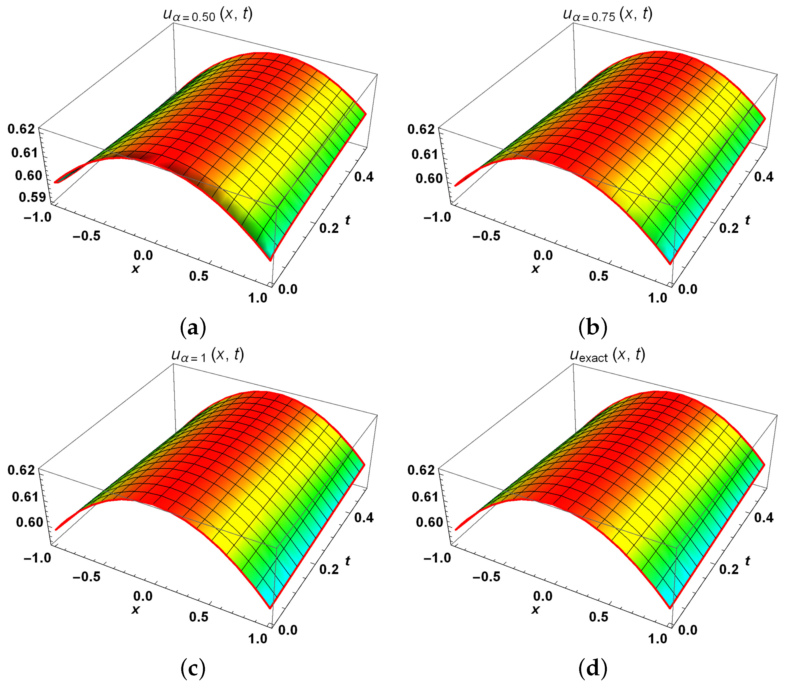
This segment presents a detailed discussion of the graphic depictions of the findings obtained through the use of SHTM. Our proposed scheme efficiently handles the time fractional TFK and TFMK problems, and provides a rapid series of results that ultimately lead to a precise solution. We have showcased the surface results of $u(x,t)$ for distinct values of time-fractional order equations in Brownian motion. The 3D results offer valuable insights into the intricate structures, movements, and relationships of our world. These findings provide valuable perspectives into the characteristics and dynamics of the model.

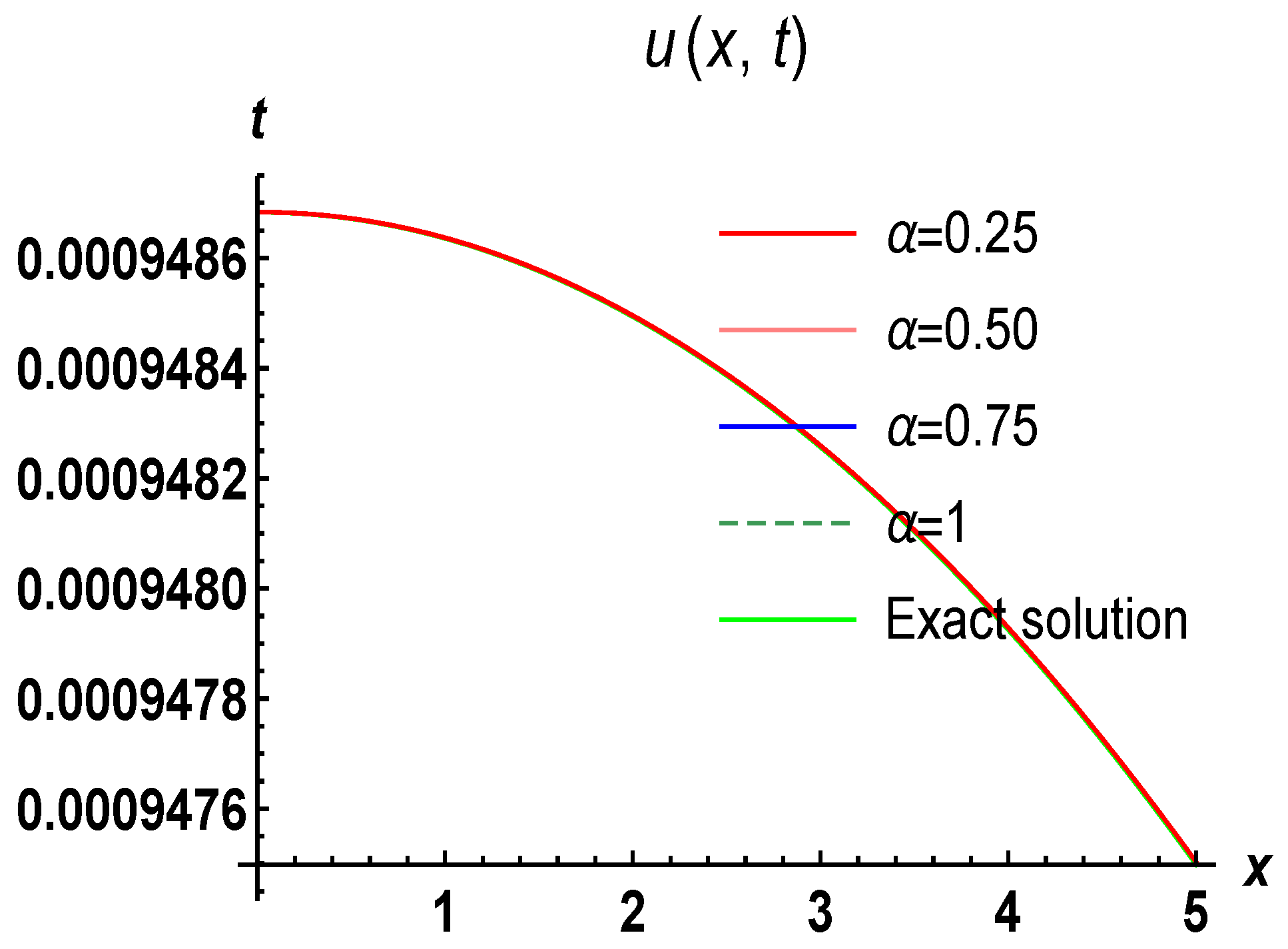
Figure 1a depicts the 3D graphical results for $\alpha =0.50$, Figure 1b depicts the 3D graphical results for $\alpha =0.75$, Figure 1c depicts the 3D graphical results for $\alpha =1$, and Figure 1d depicts the 3D graphical results for precise results. The value of $u(x,t)$ reduces within the specified range of the spatial variable x and time t in Section 5.1. Figure 2 demonstrates the visual error of $u(x,t)$ at $0\le x\le 0.5$ and $0\le t\le 2$ when $\alpha =0.25$ (red line), $\alpha =0.50$ (pink line), $\alpha =0.75$ (blue line), $\alpha =1$ (dashed line), and the precise results (green line).

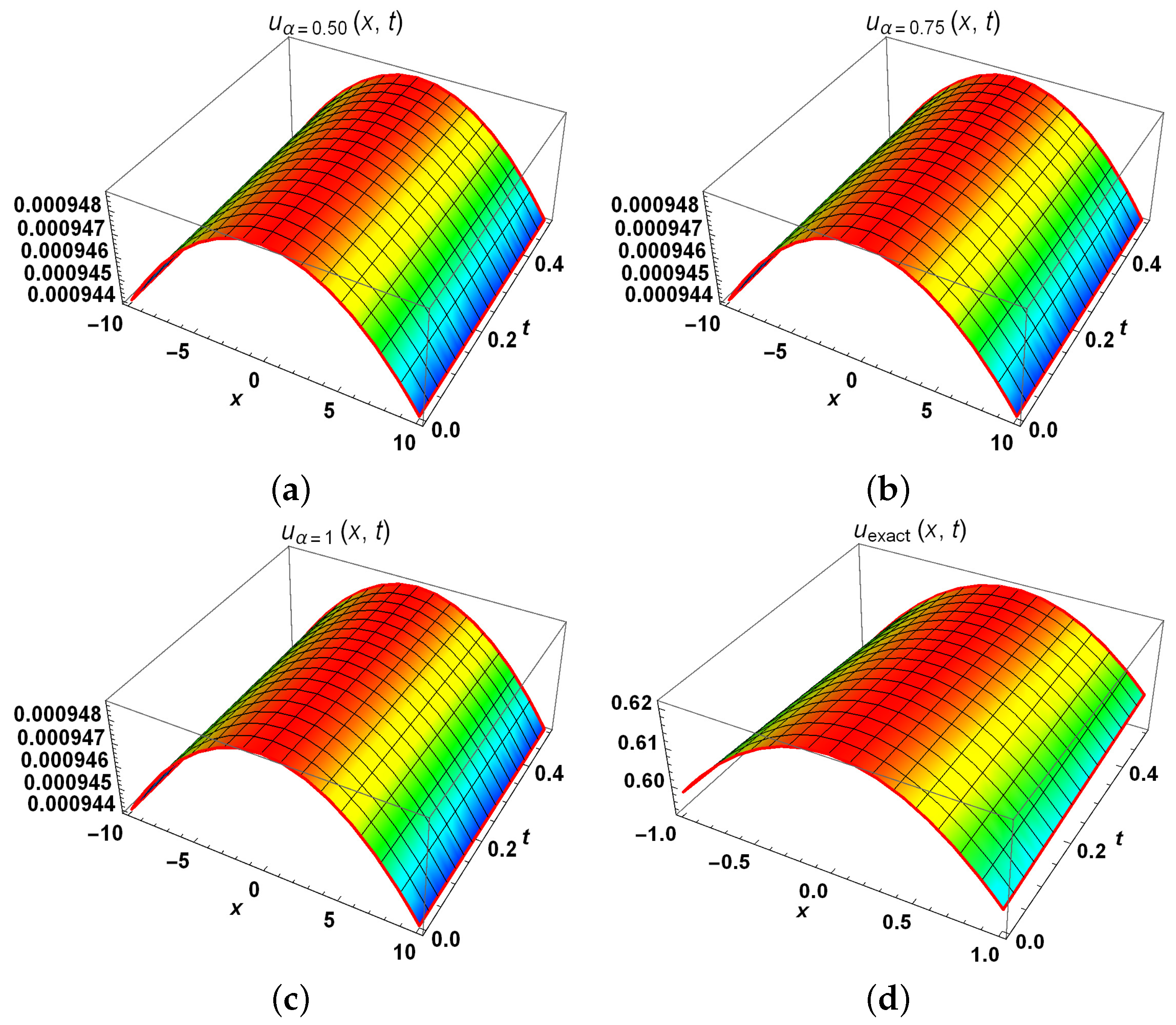
Figure 3a depicts the 3D graphical results for $\alpha =0.50$, Figure 3b depicts the 3D graphical results for $\alpha =0.75$, Figure 3c depicts the 3D graphical results for $\alpha =1$, Figure 3d depicts the 3D graphical results for the precise results. The value of $u(x,t)$ reduces within the specified range of the spatial variable x and time t in Section 5.2. Figure 4 demonstrates the graphical error of $u(x,t)$ at $0\le x\le 0.5$ and $0\le t\le 2$ when $\alpha =0.25$ (red line), $\alpha =0.50$ (pink line), $\alpha =0.75$ (blue line), $\alpha =1$ (dashed line), and the precise results (green line). The 3D visuals give a broad concept of the analysis of data, image exhibits, the interaction between humans and computers, as well as various additional aspects of engineering and scientific domains. We show that it does not require many iterations to obtain an approximate solution to a fractional problem.

Table 1. A comparative analysis of the exact results and SHTM results at different fractional orders.

x	t	SHTM Results	SHTM Results	SHTM Results	Precise Results
		$\mathbf{\alpha }=\mathbf{0}.\mathbf{50}$	$\mathbf{\alpha }=\mathbf{0}.\mathbf{75}$	$\mathbf{\alpha }=\mathbf{1}$
0.25	0.1	0.620501	0.62025	0.620053	0.620053
	0.3	0.620734	0.620664	0.620475	0.620475
	0.5	0.620760	0.62088	0.620811	0.620810
0.50	0.1	0.616948	0.616285	0.615854	0.615854
	0.3	0.617843	0.617322	0.616777	0.616777
	0.5	0.618329	0.618060	0.617616	0.617615
0.75	0.1	0.610484	0.609421	0.608763	0.608763
	0.3	0.612027	0.611064	0.610171	0.610171
	0.5	0.612965	0.612311	0.611500	0.611498
1	0.1	0.601218	0.599771	0.598897	0.598897
	0.3	0.603383	0.601993	0.600768	0.600768
	0.5	0.604756	0.601993	0.602564	0.602562

shows a comparison of the exact results and the SHTM results in different fractional orders. The proposed strategy shows that only two iterations provides incredible alignment towards the precise results. It is evident that by using more parameters, the accuracy of the findings can be significantly improved, and the errors will converge to zero. By extending the value of $\alpha$, nonlinear results are impacted, even though the wave amplitude is reduced. The graphical representations in 2D and 3D show that the results are completely consistent, indicating that our proposed scheme can handle TFK and TFMK problems.

7. Conclusions

In the present study, we investigated the series solution of TFK and TFMK problems by employing a semi-analytical technique under Caputo fractional order derivatives. The derived results were shown through an easy computational series that produced precise results very swiftly. We also verified the results of our general technique using two types of graphs in two-dimensional and three-dimensional styles with various fractional values. In this proposed scheme, we did not require any hypothesis or restriction on variables during the development of this strategy. The symmetry design was a crucial element of the TFK and TFMK models, and it was evident in the graphs that the solution exhibited a symmetrical structure. The approach we utilized was highly efficient and reliable when dealing with fractional-order challenges. The most significant advantage of SHTM was the reduction in the amount of time required for computation. The Shehu homotopy transform method (SHTM) was utilized to analyze the approximate solution for fractional problems as a series solution. This method has the potential to be applied to several nonlinear fractional challenges in engineering and science in future research.

References

- Uchaikin, V.V. Fractional derivatives for physicists and engineers. In Nonlinear Physical Science; Higher Education Press: Beijing, China, 2013; Volume I. [Google Scholar]
- Pang, G.; Lu, L.; Karniadakis, G.E. fPINNs: Fractional physics-informed neural networks. SIAM J. Sci. Comput. 2019, 41, A2603–A2626. [Google Scholar] [CrossRef]
- Kumar, S.; Kumar, A.; Samet, B.; Gómez-Aguilar, J.; Osman, M. A chaos study of tumor and effector cells in fractional tumor-immune model for cancer treatment. Chaos Solit. Fractals 2020, 141, 110321. [Google Scholar] [CrossRef]
- Cuesta, E.; Kirane, M.; Malik, S.A. Image structure preserving denoising using generalized fractional time integrals. Signal Process. 2012, 92, 553–563. [Google Scholar] [CrossRef]
- Miller, K.S.; Ross, B. An Introduction to the Fractional Calculus and Fractional Differential Equations; Wiley: New York, NY, USA, 1993. [Google Scholar]
- Herrmann, R. Fractional Calculus: An Introduction for Physicists; World Scientific: Singapore, 2011. [Google Scholar]
- Jafari, H.; Nazari, M.; Baleanu, D.; Khalique, C.M. A new approach for solving a system of fractional partial differential equations. Comput. Math. Appl. 2013, 66, 838–843. [Google Scholar] [CrossRef]
- Alquran, M.; Ali, M.; Alsukhour, M.; Jaradat, I. Promoted residual power series technique with Laplace transform to solve some time-fractional problems arising in physics. Results Phys. 2020, 19, 103667. [Google Scholar] [CrossRef]
- Zhang, Y. A finite difference method for fractional partial differential equation. Appl. Math. Comput. 2009, 215, 524–529. [Google Scholar] [CrossRef]
- Gaber, A.; Aljohani, A.; Ebaid, A.; Machado, J.T. The generalized Kudryashov method for nonlinear space–time fractional partial differential equations of Burgers type. Nonlinear Dyn. 2019, 95, 361–368. [Google Scholar] [CrossRef]
- Zheng, B.; Wen, C. Exact solutions for fractional partial differential equations by a new fractional sub-equation method. Adv. Differ. Equ. 2013, 2013, 1–12. [Google Scholar] [CrossRef]
- Rezazadeh, H.; Korkmaz, A.; Eslami, M.; Vahidi, J.; Asghari, R. Traveling wave solution of conformable fractional generalized reaction Duffing model by generalized projective Riccati equation method. Opt. Quantum Electron. 2018, 50, 1–13. [Google Scholar] [CrossRef]
- Aksoy, E.; Kaplan, M.; Bekir, A. Exponential rational function method for space–time fractional differential equations. Waves Random Complex Media 2016, 26, 142–151. [Google Scholar] [CrossRef]
- Tariq, H.; Akram, G. New approach for exact solutions of time fractional Cahn–Allen equation and time fractional Phi-4 equation. Phys. A Stat. Mech. Its Appl. 2017, 473, 352–362. [Google Scholar] [CrossRef]
- Mishra, N.K.; AlBaidani, M.M.; Khan, A.; Ganie, A.H. Two novel computational techniques for solving nonlinear time-fractional laxs korteweg-de vries equation. Axioms 2023, 12, 400. [Google Scholar] [CrossRef]
- Aniqa, A.; Ahmad, J. Soliton solution of fractional sharma-tasso-olever equation via an efficient (G’/G)-expansion method. Ain Shams Eng. J. 2022, 13, 101528. [Google Scholar] [CrossRef]
- Kaya, D.; Al-Khaled, K. A numerical comparison of a Kawahara equation. Phys. Lett. A 2007, 363, 433–439. [Google Scholar] [CrossRef]
- Daşcıoğlu, A.; Ünal, S.Ç. New exact solutions for the space-time fractional Kawahara equation. Appl. Math. Model. 2021, 89, 952–965. [Google Scholar] [CrossRef]
- Başhan, A. An efficient approximation to numerical solutions for the Kawahara equation via modified cubic B-spline differential quadrature method. Mediterr. J. Math. 2019, 16, 14. [Google Scholar] [CrossRef]
- Kawahara, T. Oscillatory solitary waves in dispersive media. J. Phys. Soc. Jpn. 1972, 33, 260–264. [Google Scholar] [CrossRef]
- Wazwaz, A.M. New solitary wave solutions to the modified Kawahara equation. Phys. Lett. A 2007, 360, 588–592. [Google Scholar] [CrossRef]
- Sirendaoreji. New exact travelling wave solutions for the Kawahara and modified Kawahara equations. Chaos Solit. Fractals 2004, 19, 147–150. [Google Scholar] [CrossRef]
- Jin, L. Application of variational iteration method and homotopy perturbation method to the modified Kawahara equation. Math. Comput. Model. 2009, 49, 573–578. [Google Scholar] [CrossRef]
- AlBaidani, M.A.M.; Ganie, A.H.; Aljuaydi, F.; Khan, A. Application of analytical techniques for solving fractional physical models arising in applied sciences. Fract. Fract. 2023, 7, 584. [Google Scholar] [CrossRef]
- Koppala, P.; Kondooru, R. An efficient technique to solve time-fractional Kawahara and modified Kawahara equations. Symmetry 2022, 14, 1777. [Google Scholar] [CrossRef]
- Çulha Ünal, S. Approximate solutions of time fractional kawahara equation by utilizing the residual power series method. Int. J. Appl. Comput. Math. 2022, 8, 78. [Google Scholar] [CrossRef]
- Odibat, Z.Z.; Momani, S.; Xu, H. A reliable algorithm of homotopy analysis method for solving nonlinear fractional differential equations. Appl. Math. Model. 2010, 34, 593–600. [Google Scholar] [CrossRef]
- He, J.H.; Latifizadeh, H. A general numerical algorithm for nonlinear differential equations by the variational iteration method. Int. J. Numer. Methods Heat Fluid Flow 2020, 30, 4797–4810. [Google Scholar] [CrossRef]
- Rani, D.; Mishra, V.; Cattani, C. Numerical inverse laplace transform for solving a class of fractional differential equations. Int. Symmetry 2019, 11, 530. [Google Scholar] [CrossRef]
- Qureshi, S.; Kumar, P. Using Shehu integral transform to solve fractional order Caputo type initial value problems. J. Appl. Math. Comput. Mech. 2019, 18, 75–83. [Google Scholar] [CrossRef]
- Jena, S.R.; Sahu, I. A novel approach for numerical treatment of traveling wave solution of ion acoustic waves as a fractional nonlinear evolution equation on Shehu transform environment. Phys. Scr. 2023, 98, 085231. [Google Scholar] [CrossRef]
- Shah, R.; Saad Alshehry, A.; Weera, W. A semi-analytical method to investigate fractional-order gas dynamics equations by Shehu transform. Symmetry 2022, 14, 1458. [Google Scholar] [CrossRef]
- Areshi, M.; Zidan, A.; Shah, R.; Nonlaopon, K. A modified techniques of fractional-order Cauchy-reaction diffusion equation via Shehu transform. J. Funct. Spaces 2021, 2021, 1–15. [Google Scholar] [CrossRef]
- Yıldırım, A.; Koçak, H. Homotopy perturbation method for solving the space–time fractional advection–dispersion equation. Adv. Water Resour. 2009, 32, 1711–1716. [Google Scholar] [CrossRef]
- Farhood, A.K.; Mohammed, O.H. Homotopy perturbation method for solving time-fractional nonlinear variable-order delay partial differential equations. Partial Differ. Equ. Appl. Math. 2023, 7, 100513. [Google Scholar] [CrossRef]
Disclaimer/Publisher’s Note: The statements, opinions and data contained in all publications are solely those of the individual author(s) and contributor(s) and not of MDPI and/or the editor(s). MDPI and/or the editor(s) disclaim responsibility for any injury to people or property resulting from any ideas, methods, instructions or products referred to in the content. |
© 2024 by the authors. Licensee MDPI, Basel, Switzerland. This article is an open access article distributed under the terms and conditions of the Creative Commons Attribution (CC BY) license (https://creativecommons.org/licenses/by/4.0/).