Fractal Characteristics of Wind Speed Time Series Under Typhoon Climate in Southeastern China

Abstract

In fractal theory, the fractal dimension has been accepted as a quantitative parameter to measure the complexity of fluctuations and the persistence of wind speeds. Typhoons are extreme wind events that damage structures. In this study, on the basis of wind field measurements, the fractal dimension characteristics of four typhoons in southeastern China are examined. Typhoon wind speeds at different heights and locations are presented. Monofractal dimension analysis was first conducted, and the results revealed that the typhoon wind speeds were persistent, with fractal dimensions smaller than 1.5. For all four typhoons considered, with the onset of landfall, the fractal dimensions approach 1.5, indicating unpredictable trends in the time series. Multifractality is accepted to exist in the typhoon wind speed dataset, and multifractal analysis was also conducted on the basis of the measured typhoon wind speeds. The results show that the fractal parameters calculated by multifractal analysis are generally greater than those calculated via monofractal analysis. This research aims to improve the understanding of the inner dynamic characteristics of typhoon wind speeds. These fractal parameters can provide quantitative references for future typhoon simulations and predictions.

1. Introduction

As extreme weather events, typhoons seriously damage structures such as bridges, high-rise buildings, and wind turbines because of their high wind speeds, which may also result in severe losses of life and property. In 2016, for example, the super typhoon Meranti caused economic losses of approximately $2 billion in China (2024). Therefore, accurate typhoon predictions, including paths and wind speed predictions, are meaningful for reducing the number of typhoon disasters. According to existing research results obtained from measurements, the wind speeds upon landfall are highly variable and contain nonstationary components, which poses challenges in predicting the time series of typhoon wind speeds. The accurate identification of typhoon complexities at spatial and temporal scales is a key step in improving the simulation accuracies and prediction results for wind speed time series. The turbulence characteristics of typhoon wind speeds have been investigated in numerous studies on the basis of both wind field measurements [1,2,3] and numerical simulations [4,5]. Nonstationary characteristics are found in typhoon wind speeds, as shown in the literature [6,7], causing challenges in wind speed prediction. Wind prediction methods, such as physical, statistical, and artificial intelligence-based approaches, are applied to predict typhoon wind speeds by integrating key parameters into various typhoon models. For example, Fang [8] proposed an analytical model that considers the effects of terrain on the field parameters. To devise an accurate wind speed prediction model, an understanding of the physical characteristics of wind speeds is necessary. Recently some researchers have started to consider the physical characteristics of wind speed by using fractal features to determine key parameters in the Lorenz–Steno equation [9]. Results show the advantage of a fractal feature based method when used to select the key parameter in an atmospheric motion equation.

Fractals are proposed to describe self-similarity at different sizes and scales. The fractal dimension can be a noninteger that measures the irregularities of a set at different scales. A higher fractal dimension indicates a more complex and rougher shape [10,11,12]. As a type of turbulent flow, wind speeds can be described by a fractal function, and feedback information about the wind field under near-ground conditions can be extracted by the fractal method [13,14]. The monofractal or multifractal characteristics present information on such stochastic processes, and therefore have been applied to wind speed analyses in numerous studies. On the basis of wind speed data at three wind speeds, Chang [15] reported that the values of the annually averaged fractal dimensions range between 1.61 and 1.66 and are negatively related to the wind speed. However, Fortuna [16] reported that the wind speeds measured in the USA and Italy exhibit characteristics of low-dimensional chaos, with fractal dimensions of 1.19 and 1.41, respectively. Moreover, on the basis of fractal theory, different types of wind speeds, such as monsoon [17,18] and typhoon [19] wind speeds, are investigated at the 10-min, daily, hourly, and monthly time scales. In Liang’s research [20], anti-persistence in wind speed time series was found during strong winds on the basis of 10 min of wind speed data, and the fractal dimensions were proven to be different at different altitudes. However, on the basis of monthly wind speeds, fractal dimensions between 1 and 1.5 have been calculated, indicating persistence characteristics [18]. Shu [21] investigated the influence of terrain on the fractal dimensions and concluded that more complex terrain results in larger fractal dimensions and therefore greater complexity in wind speed fluctuations.

In addition to the time scale of the wind speeds, the method applied to analyze the fractal dimensions influences the fractal analysis results. The methods used for the determinations include the box-counting method [22], variation method [23], and Hurst R/S method [10]. Since multifractality in wind speeds has been demonstrated, the methods used for multifractal analysis, such as multifractal detrended fluctuation analysis (MFDFA) [24], multifractal detrended moving average (MFDMA) [25], and empirical mode decomposition (EMD) [26], which can efficiently analyze one-dimensional wind speed datasets, have been applied to good effect. The MFDFA algorithm has advantages in calculating negative q moments of short time series due to its simplicity.

Fractal theory reveals the complexity of structures in nature and mathematics through self-similarity and fractional dimensions. Fractal analyses, such as fractal dimensions, can measure the inner dynamics and nature of turbulence. Typhoon processes are hard to predict due to their high turbulence. The existing prediction methods are mainly based on the wind speed data. They hardly consider the physical characteristics of typhoon processes. In this research, fractal analyses of four typhoons are conducted based on measured wind speed data, and varying fractal dimensions are presented to quantify the complexity of the fluctuations in typhoon processes. This work can be further utilized to estimate or simulate typhoon processes in the future by providing a quantitative reference. In this research, with utilization of measured wind speed data, the fractal dimensions of four typhoon processes are analyzed. The typhoon data were first filtered using data control methods, and four typhoon processes were presented. Monofractal analysis was then conducted using a box-counting method. Then the multifractal characteristics were found in the typhoon wind speeds. Then MFDFA was conducted using data from four typhoons that were measured in southeastern China. By using MFDFA, multifractal characteristics were proven to exist in all four typhoon processes.

2. Data Sources and Processing

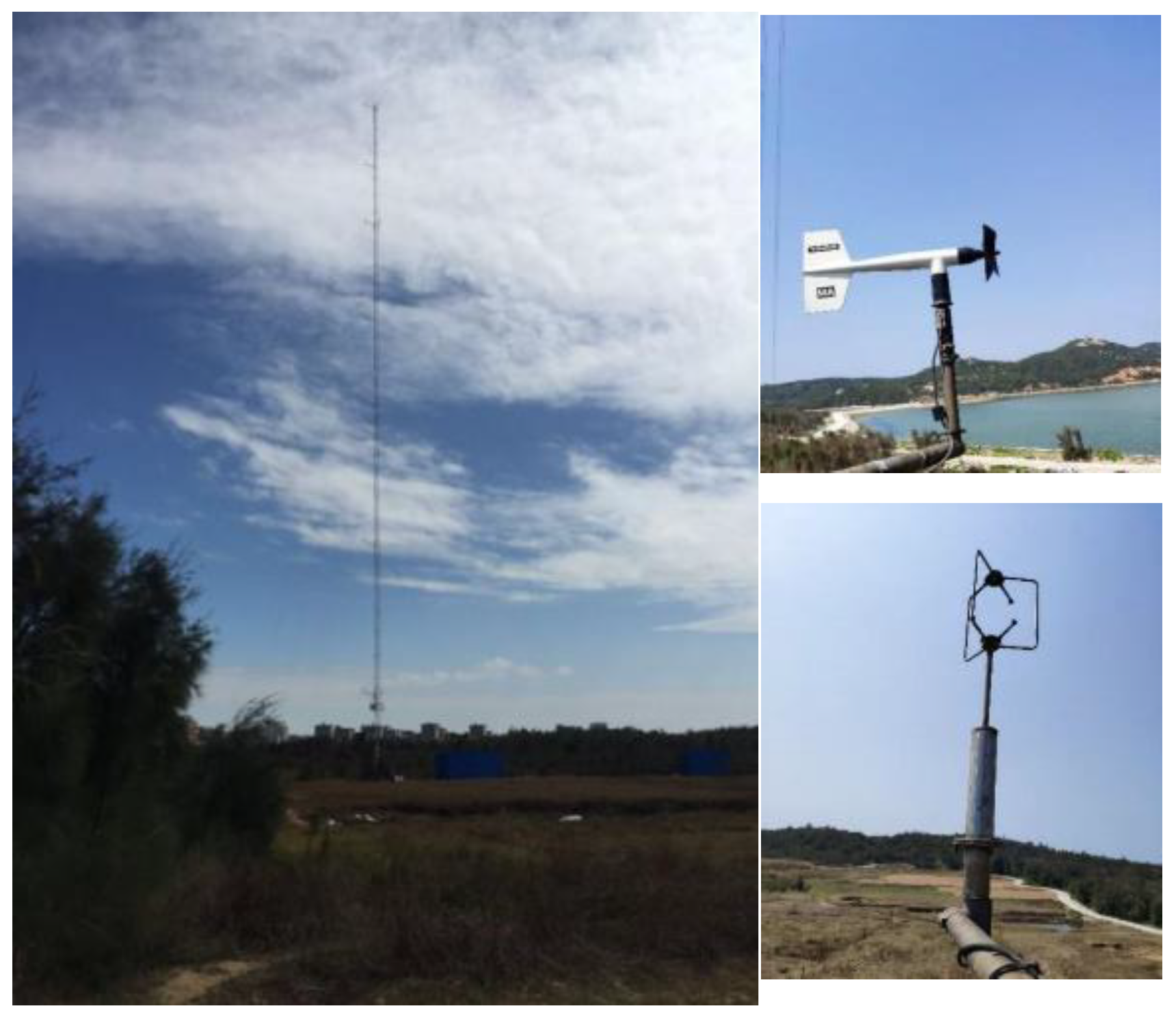
2.1. Experiment Site and Instruments

The data presented in this research are based on wind field measurements taken at two locations in Pingtan County, Fujian Province, China, as shown in Figure 1. Fujian Province is located in the southeastern coastal area of China and is rich in wind resources because of its geographical location and climate conditions. Numerous wind farms have been constructed for wind power generation. However, extreme wind events may occur, such as typhoons, which may influence the safety and stability of wind turbines [2,3]. In this research, wind field measurements were taken at two stations, as shown in Figure 1. Station 1 is located on Wangye Mountain in Pingtan County (WM Station), and Station 2 is located on Yutou Island in Pingtan County (YI Station) in Fujian Province, China, as indicated in Figure 2 and Figure 3 respectively. The WM Station is located east of the Taiwan Strait and has flat terrain on the west side and an open sea on the southern and northern sides. The monsoon-dominated wind direction is north–northeast (11.25–33.75°). The YI Station is surrounded by the sea on the north side and a small forest on the east side. Three-dimensional wind speeds were recorded with 3D sonic anemometers, as indicated in Figure 3. The 3D sonic anemometers used are high-performance Wind Master Pro devices that are produced by the UK Gill Company, with a wind speed range of 0–65 m/s, an accuracy of 0.01 m/s, a wind direction range of 0–359°, and a resolution of 0.1°. A 10 Hz output frequency is used on site, which means that one set of instantaneous 3D wind speeds is recorded every 0.1 s. The ultrasonic anemometers can work at temperatures ranging from −40 to +70 °C, and a small weather station was installed at a height of 10 m to monitor the working temperatures of the ultrasonic anemometers with a thermometer accuracy of 0.01 °C. Identification codes are generated automatically to be used as a reference for data quality control. When the data are unstable or out of range, they are flagged as 0 in the recorded data. The bad or invalid data points are eliminated and then reconstructed using the multiple truncation variance data control method [2]. For Station WM, 3D sonic anemometers were installed at heights of 10 m, 25.87 m, and 31.87 m, whereas they were installed at heights of 10 m, 80 m, and 100 m for Station YI, as shown in Figure 2 and Figure 3.

Four typhoon events were recorded from 2016 to 2019 at the two stations. Typhoons Nesat and Haitang were recorded in 2016 at the WM Station, and Typhoons Maria and Bailu were recorded at the YI Station. Detailed descriptions of the typhoon landfall times and measurement heights are provided in

Table 1. Detailed description of typhoon landfall information.

Typhoon	Landing time	Station	Measurement Height	Maximum Wind Speed at Height 10 m
Nesat	2016.07.29–2016.07.30	Wangye Shan Island	10 m, 25.87 m, 31.87 m	37.8 m/s
Haitang	2016.07.30–2016.07.31	Wangye Shan Island	10 m, 25.87 m, 31.87 m	25.4 m/s
Maria	2018.07.11–2018.07.11	Yutou Island	10 m, 80 m, 100 m	26.13 m/s
Bailu	2019.08.23–2019.08.24	Yutou Island	10 m, 80 m, 100 m	25.69 m/s

. The ultrasonic anemometers were installed on wind towers at heights of 10 m, 25.87 m, and 31.87 m at the WM Station and at heights of 10 m, 80 m, and 100 m at the YT Station. Typhoon Nesat made landfall in Fuqing, China, at 06:00 on July 30, 24.5 km away from the measurement site, and the maximum measured 10-min mean wind speed was 37.8 m/s. Typhoon Haitang made landfall after Typhoon Nesat within 24 h at the same position, with a maximum measured 10-min mean wind speed of 25.4 m/s. The landfall events of the two typhoons are shown in Figure 4. Typhoon Maria made landfall at Lianjiang, Fujian Province, China, at 09:10 on July 11, with a maximum wind speed of 42 m/s in the center; wind speeds were recorded at the measurement site. Typhoon Bailu made landfall in Dongshan County in Fujian Province at 7:25 am on 25 August 2019, with a wind speed of approximately 25 m/s near the center. Even though the measurement site is located 278 km away from the center of the landfall location, the maximum 10-min wind speed approached 25.69 m/s because of the low pressure. The landfall events for Typhoons Maria and Bailu are shown in Figure 5.

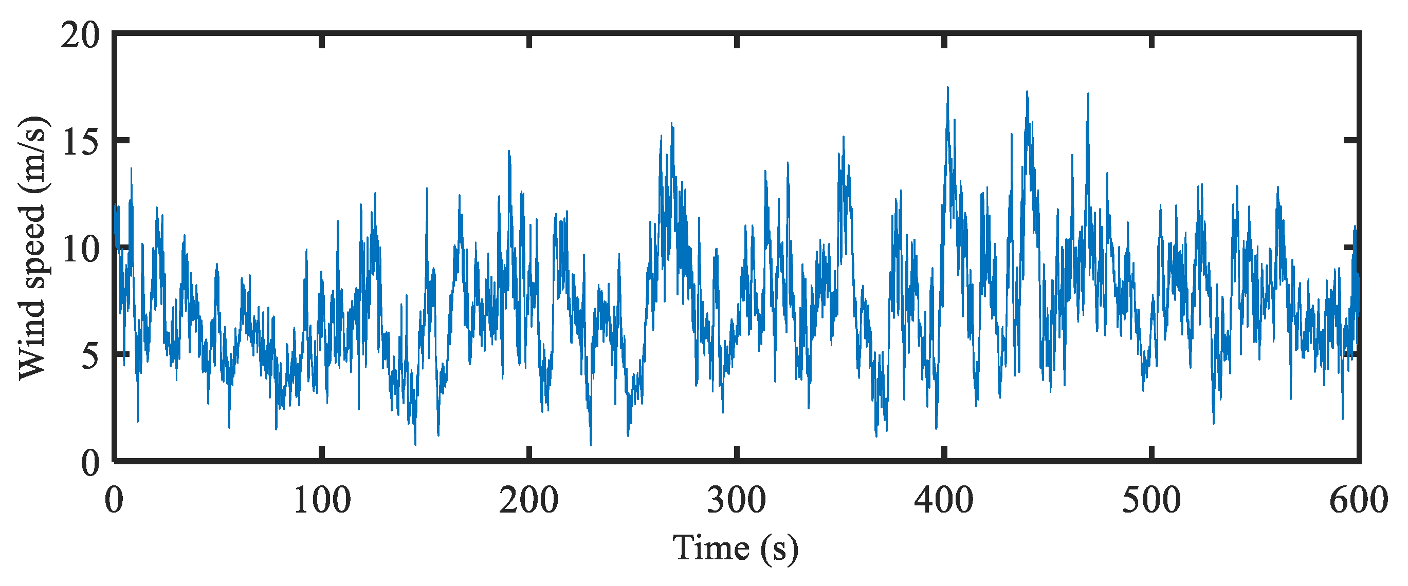
2.2. Data Control and Filtering

During wind field observations, the three-dimensional wind speeds dynamically change over time. Therefore, the obtained wind speed data may contain invalid or unreasonable points, which are usually caused by the influence of the instrument itself or by the external environment, such as instrument design defects, rainstorms, lightning, wind radiation impacts, and voltage instability. Therefore, to ensure the reliability of the experimental data, a data quality control method was applied to filter invalid points from the typhoon data. First, on the basis of the parallel observed data obtained from the surrounding meteorological observation stations, the reliability of the data was first determined by comparing the wind speeds observed at nearby meteorological stations. Thereafter, a multiple truncation variance method was used to determine the rationality of the original data with following steps:

Calculate the time series $du(t)$ as:

$$du(t)=u(t+2)-u(t)$$

(1)

The mean values of $du(t)$ and $d{u}^2$ can be expressed as:

$$\overline{du}={\displaystyle \frac{1}{n-2}}{\displaystyle \sum _{i=1}^{n-2}du(t)}, \overline{d{u}^2}={\displaystyle \frac{1}{n-2}}{\displaystyle \sum _{i=1}^{n-2}du{(t)}^2}$$

(2)

The truncation variance can be expressed as follows:

$$\sigma =\overline{d{u}^2}-{\overline{du}}^2$$

(3)

The criterion for detecting invalid data can be defined as:

$$\Delta =c\cdot {\sigma }^{0.5}$$

(4)

In this research, $u(t)$ represents the wind speed at the tth time point. In Equation (4), c = 4, which means that when the absolute value of the difference between the mean value of the sample points and the total sample is greater than 4 times the standard deviation, the point is determined to be unreasonable data and in need of modification. The modification process can be described as follows:

$$u^{(3)}={\displaystyle \frac{1}{4}}(u_{t+1}^{(2)}+2u_{t+2}^{(2)}+u_{t+3}^{(2)})$$

(5)

where $u^{(1)}$ is the median value of the sample points $u(t)$~$u(t+4)$ and $u^{(2)}$ is the median value of the sample points $u_{t+1}^{(1)}$~$u_{t+3}^{(1)}$. On the basis of the original measured data and data control processes, the 10-min wind speeds and directions for the considered typhoons are presented in Figure 6.

3. Fractal Analysis

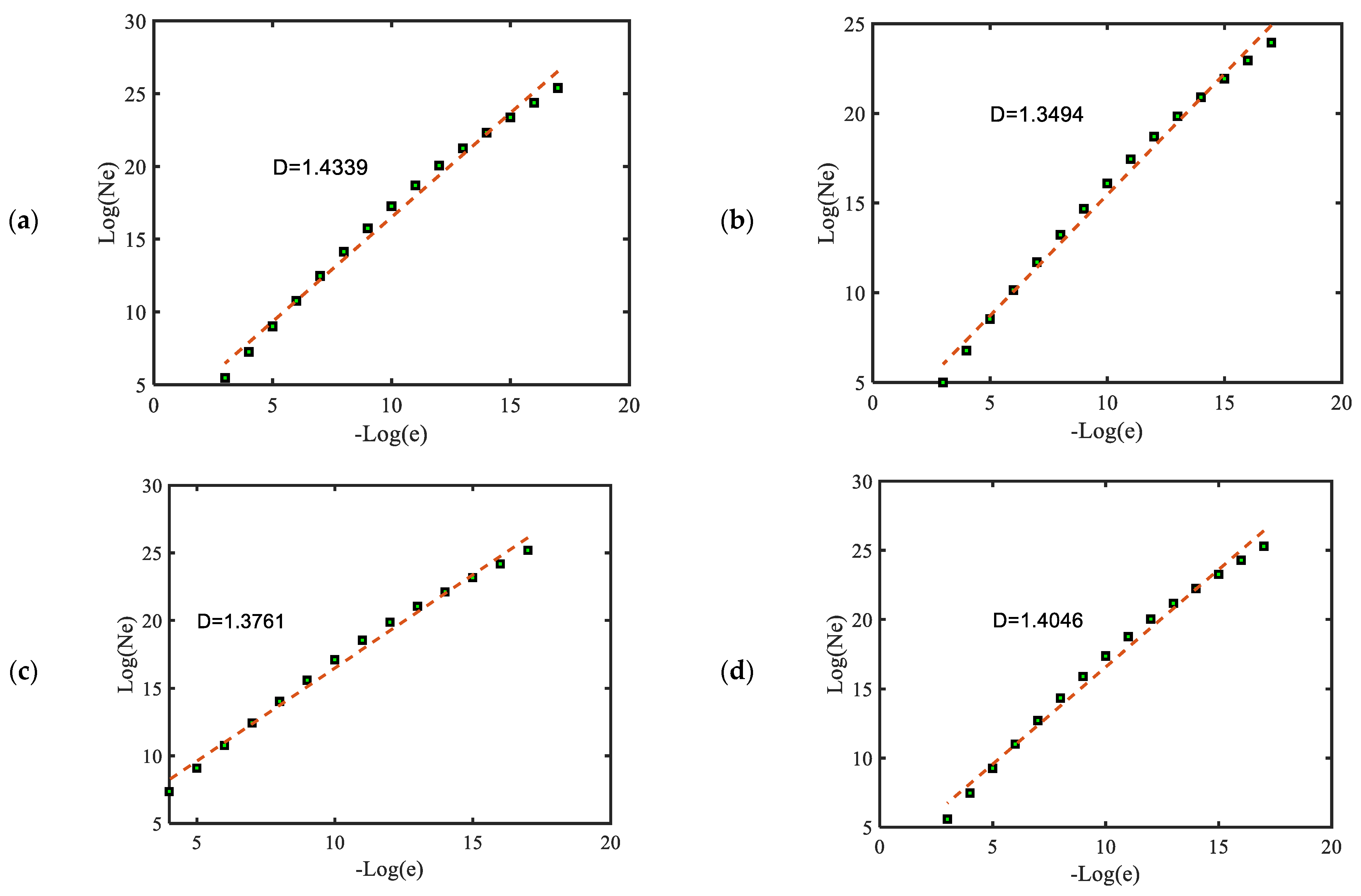
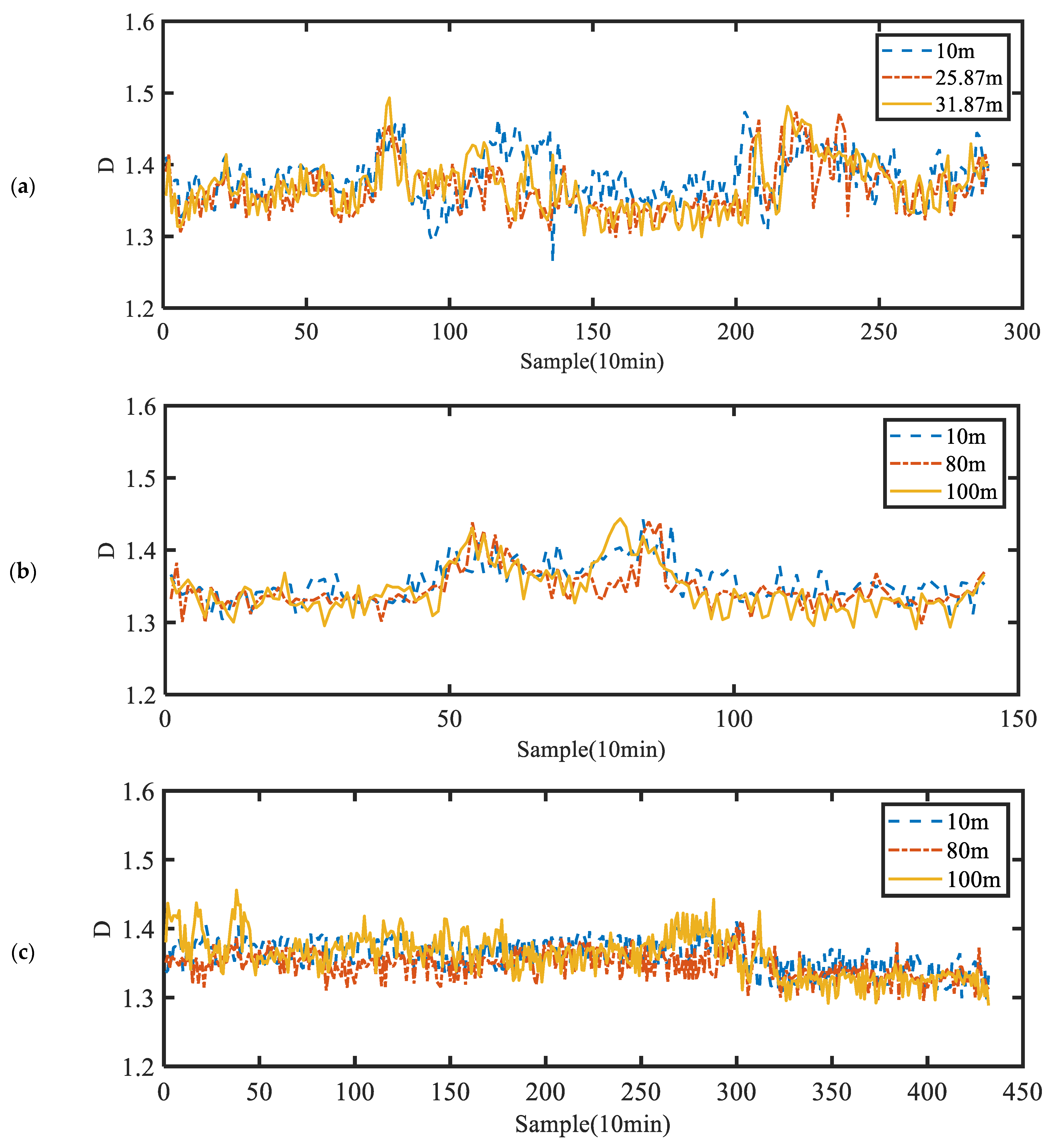
3.1. Box-Counting Method

Fractal theory, introduced by Mandelbrot, provides a framework for understanding complexity through items that exhibit self-similarity both locally and globally. The fractal dimension is a key metric for quantifying this complexity. The fractal dimension can reflect the changes in the topological measurements of a physical set across different scales [27]. Given that wind is one of the most complex turbulent phenomena in nature, analyzing its fractal dimension offers a quantitative way to assess the irregularity of wind time series, making it a valuable tool for studying turbulent behaviors, especially for typhoon wind speeds, which have been proven to have more obvious turbulent characteristics. Currently, various methods have been employed to estimate fractal dimensions, including power spectrum analysis, wavelet transforms, root mean square calculations, R/S analysis, box counting, and variance methods [10,22,27]. Among these methods, the box-counting method is particularly popular for fractal analyses of time series because of its simplicity and ease of automation. The box-counting method involves placing the time series in grids and then calculating the number of nonoverlapping boxes that can cover all of the time series. Mathematically, this can be described as follows:

$$D={\lim }_{r\to 0}{\displaystyle \frac{\log N(r)}{\log (1/r)}}$$

(6)

where D is the fractal dimension and N (r) is the number of small square grids with width r that are needed to cover the entire time series. The Hurst exponent is related to the fractal dimension as (Harrouni et al., 2009 [28]):

$$H=2-D$$

(7)

Since wind is a typical complex turbulent phenomenon in nature, the values of the fractal dimension or Hurst exponent of the wind speeds can provide hidden dynamic characteristics:

• When H = 0.5 and the fractal dimension D is 1.5, the wind speed series is random and unpredictable. This is called a Brownian time series or a random walk. Time series with such characteristics are often considered white noise.
• When 0 < H < 0.5, the fractal dimension is larger than 1.5, and the wind speed series shows anti-persistence, indicating that the wind speeds have a long-term negative autocorrelation and long-term conversion between high and low in the future.
• When 0.5 < H < 1.0, the fractal dimension is between 1 and 1.5, the wind speeds have a long-term positive autocorrelation, and there is another high value for a long period of time.
• When H = 1, the fractal dimension equals 1, indicating that the wind speed is strongly predictable.

Fractal dimension analyses were conducted on the 10-min recorded wind speed data of the four typhoons considered. With a sampling frequency of 10 Hz, 6000 data points were calculated via the box-counting method for each segment. As indicated in Equation (6), the best estimation of the fractal dimension can be obtained when the box scale approaches infinity. In mathematical calculations, the fractal dimension can be calculated by a double logarithmic coordinate plot, and the slope of the graph can be estimated as the fractal dimension. Figure 7a–d show box plots of the four typhoons using 10-min wind speed series, in which green box represents the log of the total number of grids accumulating the coverage signal and red line represents the corresponding linear fitted line. The correlation coefficients of the linearly fitted curves for each sample are above 0.991, indicating that the wind speeds of the four typhoons exhibit fractal behavior. As reported in the previous section, the full typhoon events were recorded. Therefore, in this section, fractal dimensions were calculated for each 10-min segment on the basis of the recorded data points, as shown in Figure 4. Notably, because Typhoon Haitang closely followed Typhoon Nesat, the time series of the two typhoons are plotted in the same figure. Figure 8a–c shows the fractal dimension series of Typhoons Nesat and Haitang (24-h data), Typhoon Bailu (72-h data), and Typhoon Maria (24-h data) at different heights. As shown in Figure 7, the fractal dimensions of the four typhoons range between 1 and 1.5, indicating the persistence of the wind speeds. For all four typhoons, the fractal dimensions at lower heights are greater. Generally, stronger typhoons have greater complexity and unpredictability in terms of wind speed; therefore, Typhoon Nesat generally had the strongest fractal dimensions with the highest wind speeds. The fractal dimensions of Typhoons Nesat and Haitang are between 1.2641 and 1.4933. The maximum point can be seen at the 79th segment at a height of 10 m. Compared with the wind speed history shown in Figure 6, it represents the approach to the landfall point of Typhoon Nesat at 03:50 am on 30th July. The other maximum point, 1.47, occurs at the 203^rd segment, which is near the landfall of Typhoon Haitang at 2:50 am on 31st July. Owing to the typhoon’s landfall, both the wind speeds and the complexity of the wind speeds significantly increase, causing the fractal dimension to approach 1.5, indicating that the fractal characteristics of the wind speeds change from persistent to unpredictable. This phenomenon can also be observed in Figure 8c. With the approaching landfall of Typhoon Maria, the fractal dimension increases to 1.44, indicating a decrease in persistence and an increase in unpredictability. However, because the measurement site is located farther from the landfall center than those of Typhoons Nesat and Haitang were, the recorded wind speeds are relatively lower, and weak persistence still exists in the wind speed time series. These results reveal differences in the characteristics of the fractal dimensions of Typhoon Lionrock in [19], in which the fractal dimensions ranged from 1.5–1.7. The difference may be caused by the terrain conditions of the measurement sites, which have been proven to significantly affect the inner dynamics of wind speeds [21].

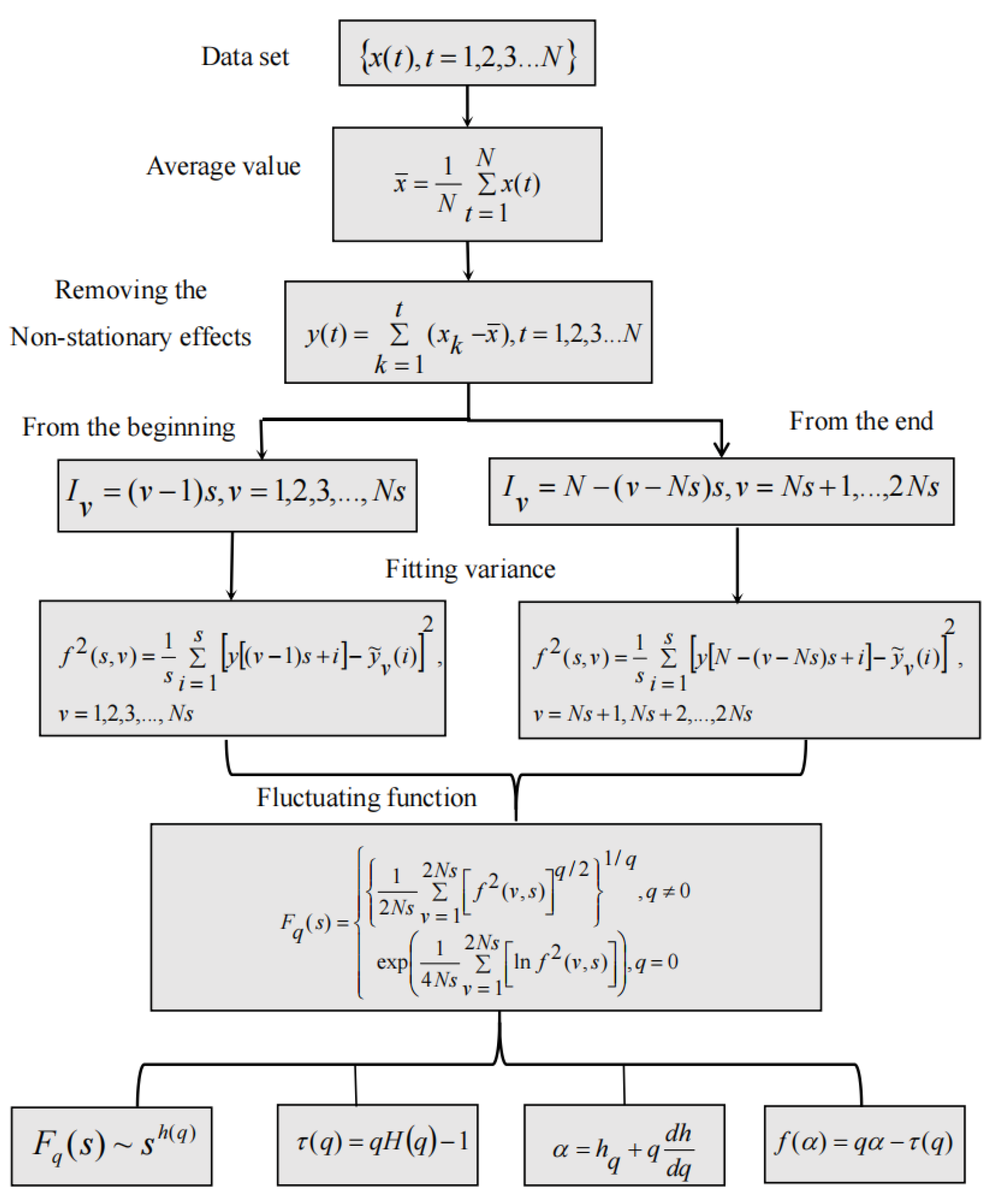
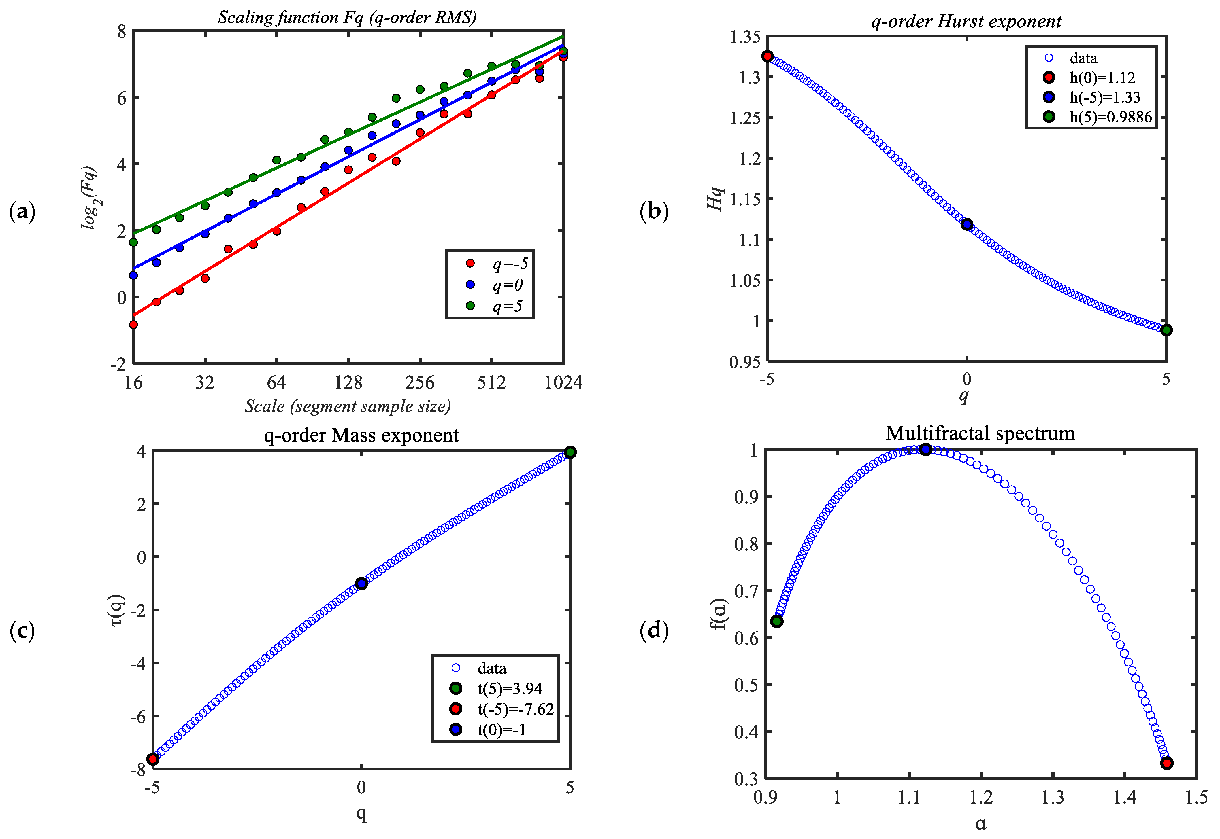
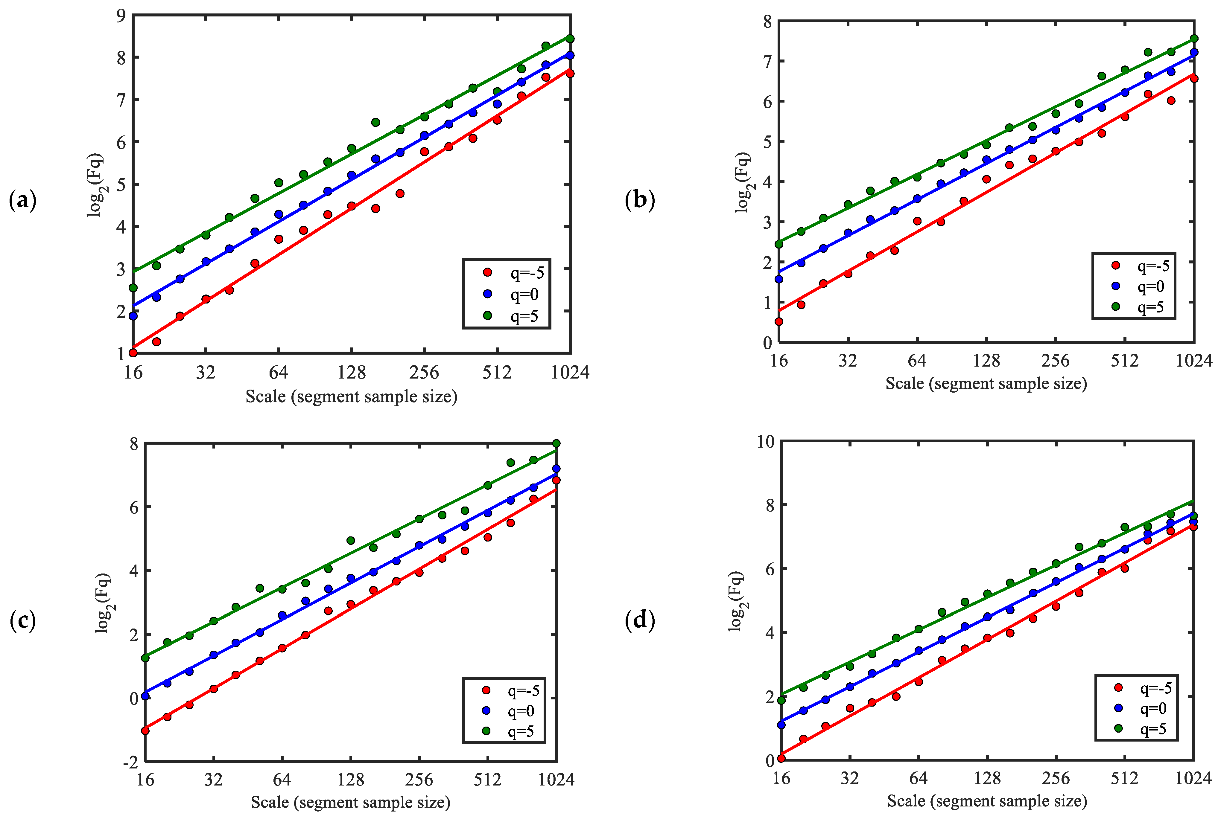
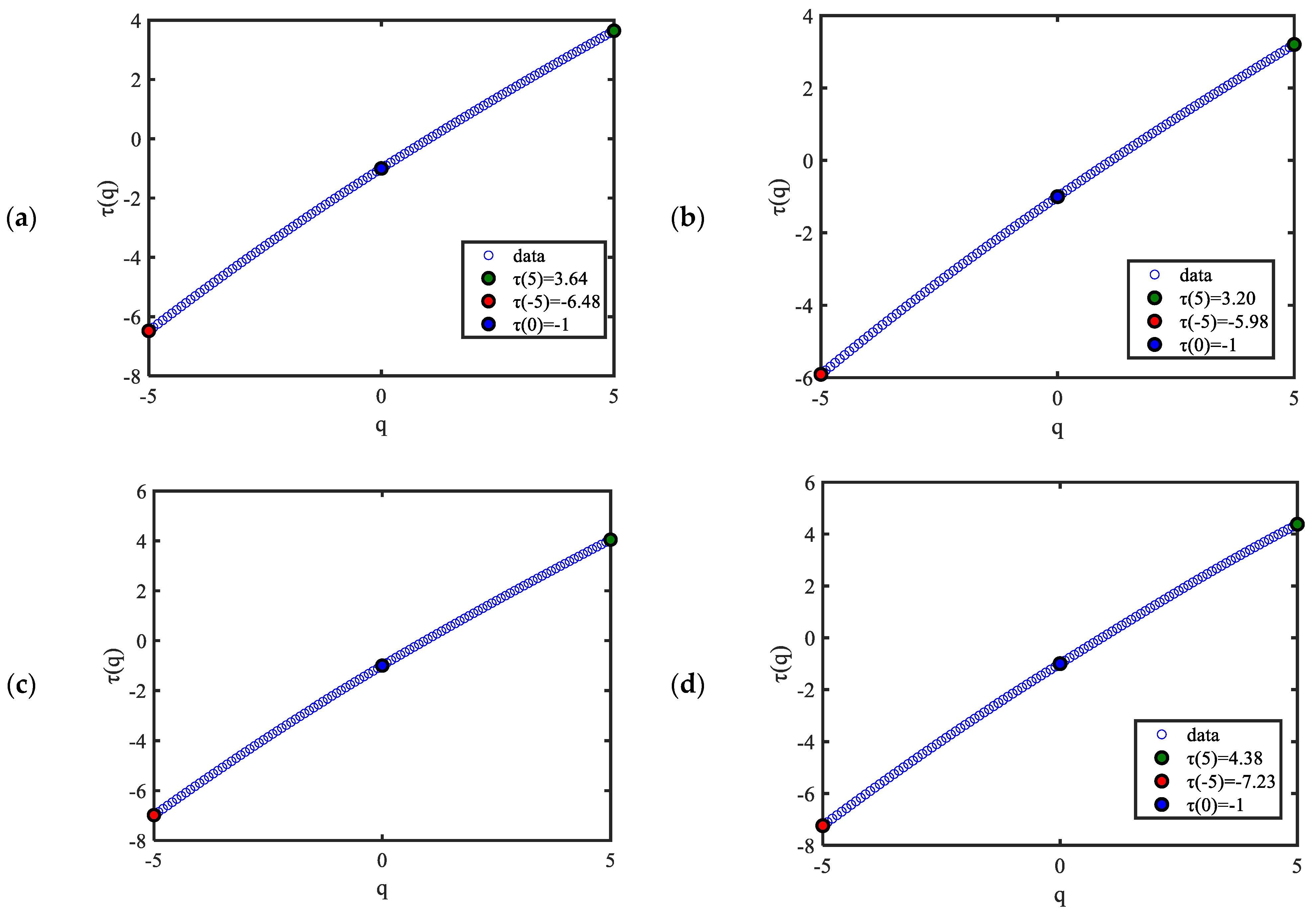
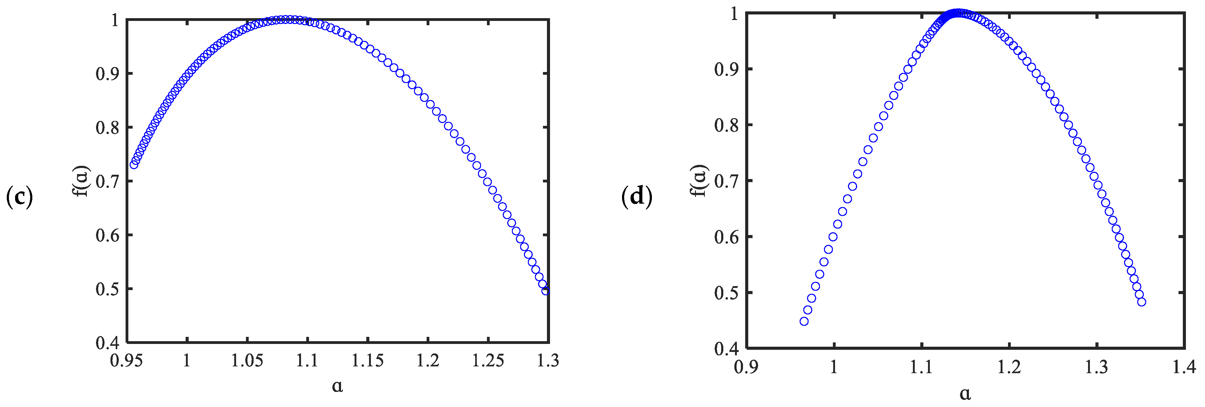
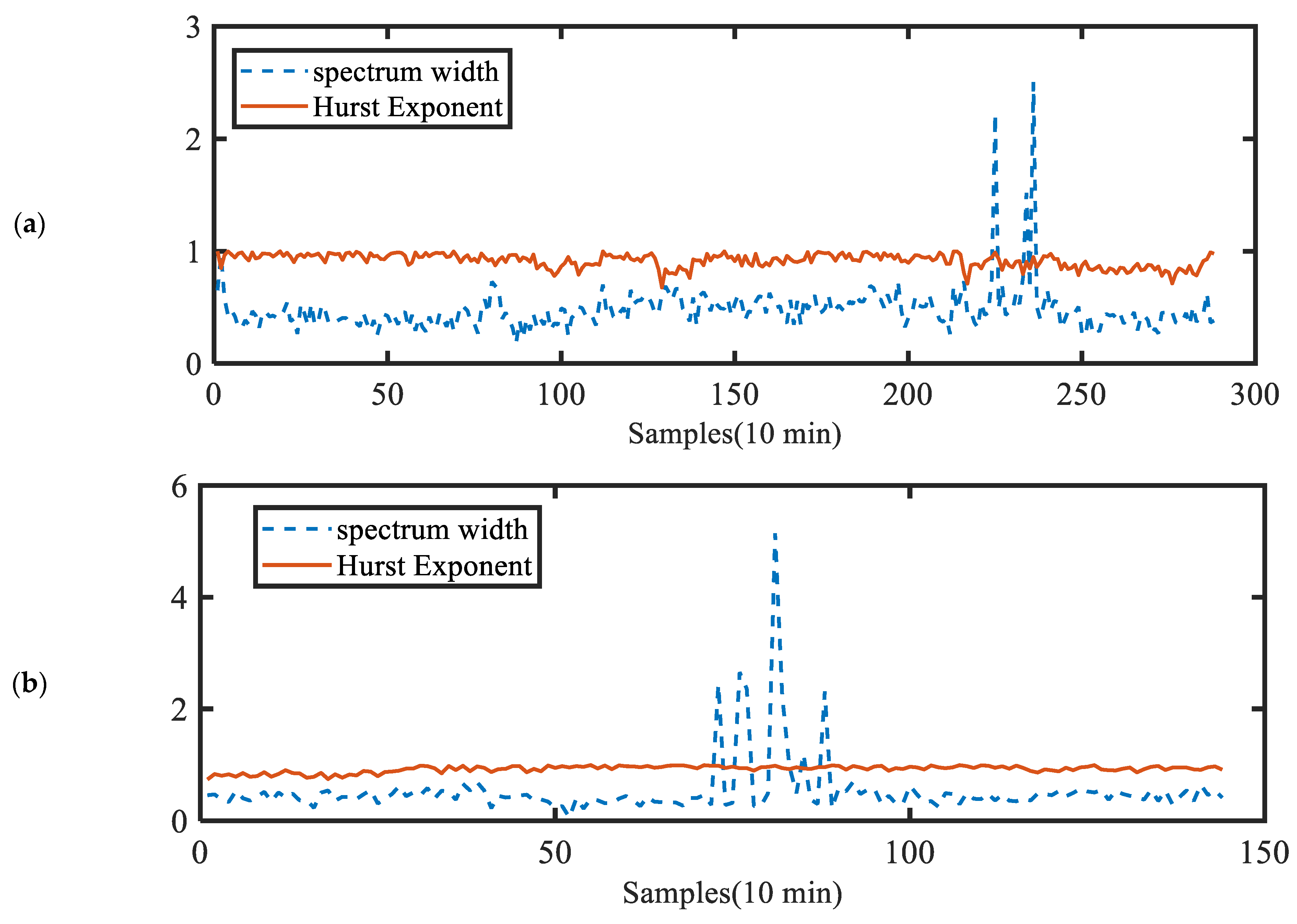
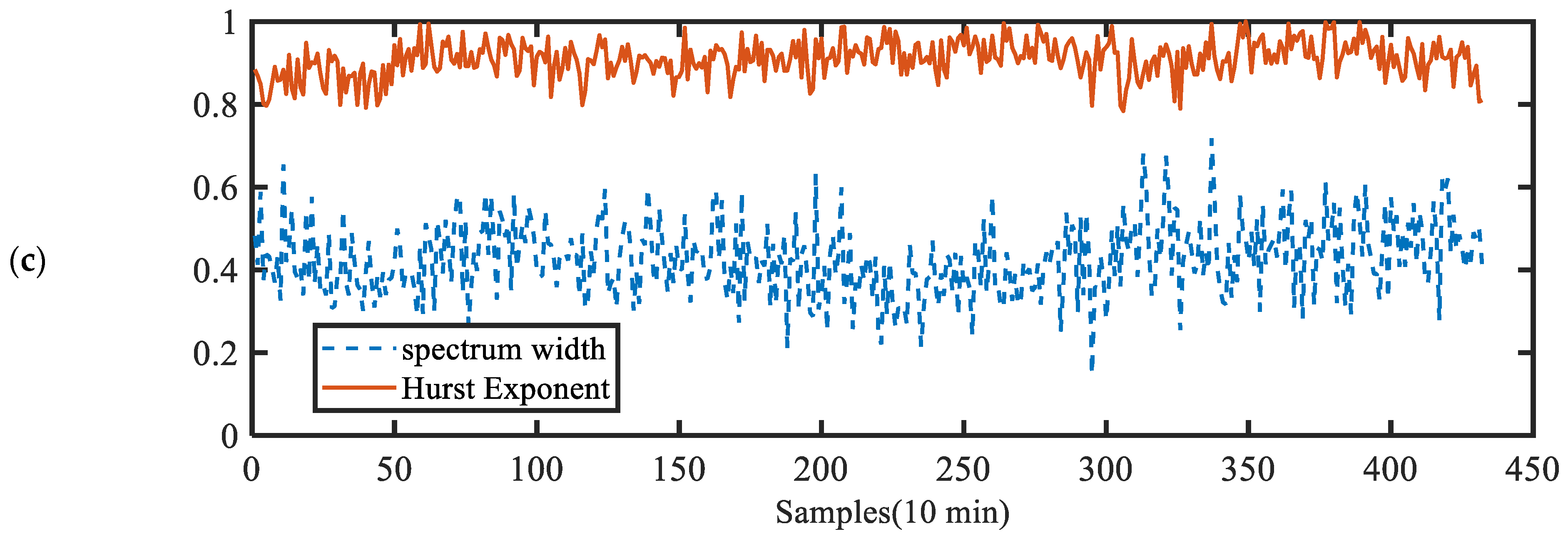
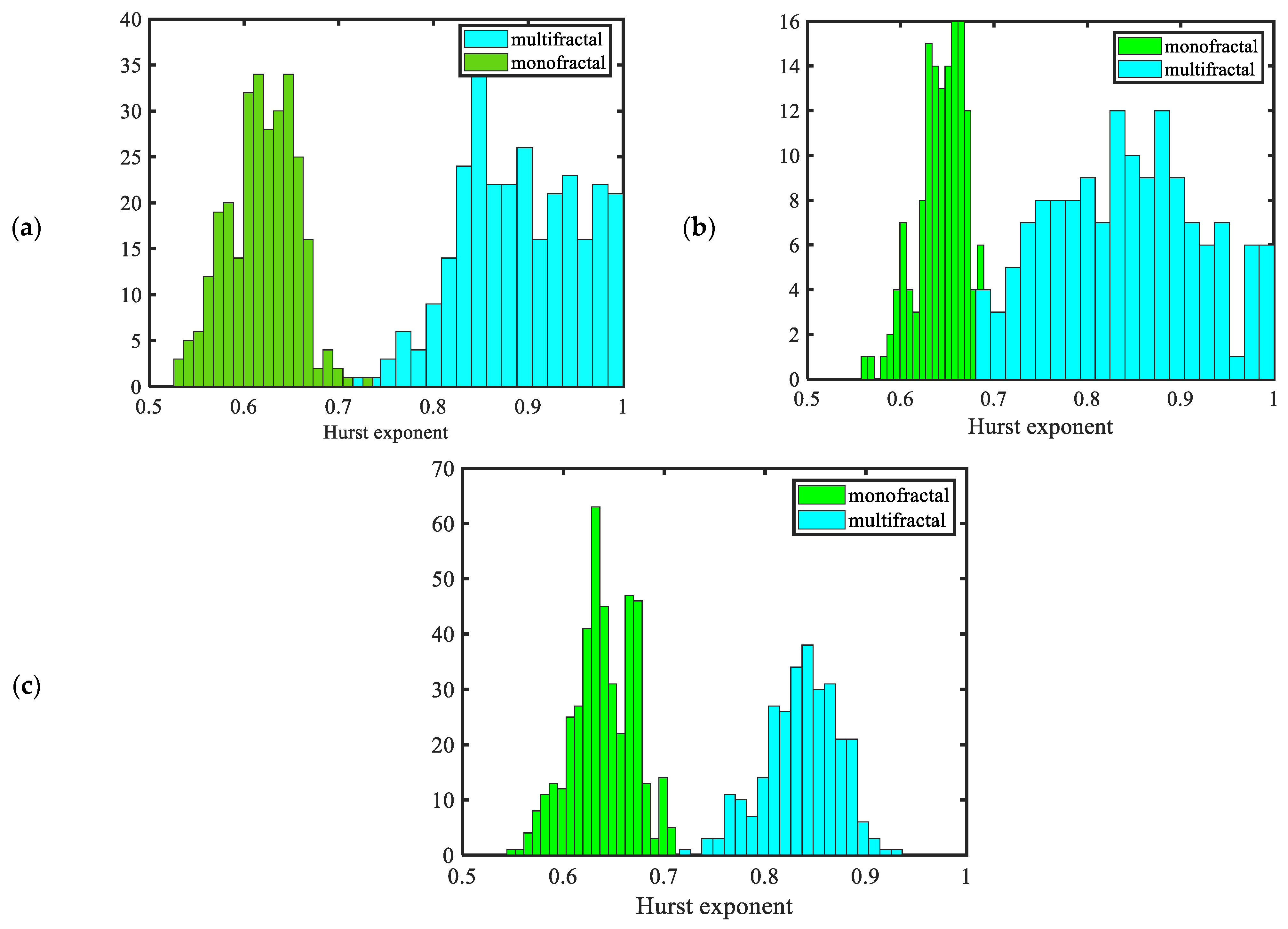
3.2. Multifractal Analysis: Multifractal Detrended Fluctuation Analysis (MFDFA)

Research has shown that a single fractal dimension might not be adequate to describe the complex behavior of wind speeds, especially for extreme weather events. Therefore, descriptions that use multiple fractal dimensions are necessary. Monofractal analysis assumes that the complexity of the system is consistent across all scales, while multifractal analysis describes the multi-scale characteristics of the system through a series of fractal dimensions (or multifractal spectrum), which can capture the heterogeneity of different scales in the system more carefully. Accordingly, multifractal detrended fluctuation analysis was applied to determine the temporal scaling properties of the wind speed series. The description of multifractal analysis is as follows:

Considering a nonstationary time series, $\left\{x(t),t=1,2,3\dots N\right\}$, the trajectory or profile preserves the variability of the time series while simultaneously reducing noise by removing the nonstationary effects as:

$$y(t)={\displaystyle \sum _{k=1}^t(x_k-}\overline{x}),t=1,2,3\dots N;\overline{x}={\displaystyle \frac{1}{N}}{\displaystyle \sum _{t=1}^{N}x(t)}$$

(8)

The trajectory y(t) is then divided into Ns nonoverlapping equal-length intervals from the beginning and end of the time series. Therefore, 2Ns nonoverlapping time series can be obtained with $N_s=\mathrm{int}(N/S)$. The vth element in the time series can be denoted as $\left\{y(I_v+t),t=1,2,\dots ,s\right\}$ when v = 1,2… Ns,

$$I_v=\left\{\begin{array}{c}(v-1)s,v=1,2,3,\dots ,Ns\\ N-(v-Ns)s,v=Ns+1,Ns+2,\dots ,2Ns\end{array}\right.$$

(9)

The variance is calculated from (5) for the two sets of partitions [13].

$$f^2(s,v)=\left\{\begin{array}{c}{\displaystyle \frac{1}{s}}{\displaystyle \sum _{i=1}^s}{\left[y\left[(v-1)s+i\right]-{\tilde{y}}_v(i)\right]}^2,v=1,2,3,\dots ,Ns\\ {\displaystyle \frac{1}{s}}{\displaystyle \sum _{i=1}^s}{\left[y\left[N-(v-Ns)s+i\right]-{\tilde{y}}_v(i)\right]}^2,v=Ns+1,Ns+2,\dots ,2Ns\end{array}\right.$$

(10)

where ${\tilde{y}}_v(i)$ is the fitting polynomial for the vth time series. Finally, the qth-order fluctuation, $F_q(s)$, is calculated from the average of all the partitions.

$$F_q(s)=\left\{\begin{array}{c}{\left\{{\displaystyle \frac{1}{2Ns}}{\displaystyle \sum _{v=1}^{2Ns}{\left[f^2(v,s)\right]}^{q/2}}\right\}}^{1/q},q\ne 0\\ \exp \left({\displaystyle \frac{1}{4Ns}}{\displaystyle \sum _{v=1}^{2Ns}\left[\ln f^2(v,s)\right]}\right),q=0\end{array}\right.$$

(11)

For each q, the double logarithm of Fq(s)-s can be calculated, and the scaling exponents of the time series fluctuations can be determined. The multifractality of the time series is caused by different long-term correlations in the sampled time series. As described previously, monofractal analysis can be applied to the fractal dimension for a whole time series, whereas the MFDFA describes the complexity and dynamics of the entire dataset at different scales. Multifractal detrended fluctuation analysis (MFDFA) was conducted, in which four types of analyses, namely, $F_q(s)$ against log(s), the generalized Hurst exponent, the mass exponent, and the multifractal spectrum, can be used to determine the multifractality as follows:

For the long-term relationship, $F_q(s)~s^{h(q)}$, where s is the considered scale and $F_q$ is the qth-order fluctuation, negative q values represent increases in small fluctuations, and positive q values indicate increases in large fluctuations. A power-law change, namely, $F_q$ increases with the increasing power of s and can determine if there is a long-term correlation in the signal. With the use of a double logarithmic plot, when $\ln (F_q)$ linearly increases with ln (s), the slope can be calculated as the generalized Hurst exponent of the recorded time series, indicating scale dependence, which is characteristic of multifractality.

The dependence of $h(q)$ on q or the generalized Hurst exponent on q indicates that in monofractal calculations, the local trend of each segment is obtained from fitting the variance calculation of each segment. Therefore, the trend is unchanged when the scaling is unchanged, namely, $h(q)$ is independent of q. However, for time series with multifractal features, the dependence of h on q is caused by fluctuations at large scales. For a large positive q value, the least squares fitting result has a large deviation, so the variance is large and the h(q) value is small, whereas for a negative q value, the variance is small and the $h(q)$ value is large. In general, for monofractal datasets, all scales have an exponent, whereas for multifractal time series, $h(q)$ monotonically decreases with increasing q.

The qth-order mass exponent with $\tau (q)$ vs. q indicates that if $\tau (q)$ varies linearly with changes in q, the time series can be considered monofractal, whereas it is multifractal if it shows a nonlinear tendency [14]. Notably, both the changes in $\tau (q)$ and $H(q)$ can provide evidence of a multifractal sequence. In Kantelhardt’s research, the relationship between the two parameters can be expressed as $\tau (q)=qH\left(q\right)-D_f$ by considering a stationary positive and normalized sequence, substituting its simplified version of the variance and standard fluctuation analysis into (6) and comparing it with the box probability for the standard multifractal formalism for the normalized series. In this expression, $D_f$ is the topological dimension of the multifractal signal. For the considered wind speed series,$D_f$ equals 1.

After α Legendre transformation, the singularity intensity function $\alpha (q)$ and the multifractal spectrum $f(\alpha )$ can be obtained. The relationship can be expressed as:

$$f(\alpha )=q\alpha -\tau (q)$$

(12)

where α is the Holder exponent and $\alpha ={\displaystyle \frac{d\tau (q)}{dq}}$. As described previously,

$$\tau (q)=qH\left(q\right)-1; \alpha =h_q+q{\displaystyle \frac{dh}{dq}}$$

(13)

A flow chart of MFDFA can be seen in the Figure 9 to show the analysis process:

The multifractal spectrum parameters include the position of max ${\alpha }_0$, width of the spectrum W and skew r. The width of the spectrum and skewness parameters can be expressed as follows [29]:

$$W={\alpha }_{\max }-{\alpha }_{\min };$$

(14)

$$r={\displaystyle \frac{{\alpha }_{\max }-{\alpha }_0}{{\alpha }_0-{\alpha }_{\min }}}$$

(15)

For a change in the q value from a negative value to a positive value, if $H(q)$ is almost constant, then the relationship between the qth-order mass exponents $\tau (q)$ and q is a straight line and the width of the multifractal spectrum is close to 0, indicating that the time dataset has single fractal characteristics. However, if H(q) changes significantly, the qth-order mass indices $\tau (q)$ and q have nonlinear relationships, and the signal has multifractal characteristics. For the skewness r, when r = 0, the fractal spectrum is symmetric. When r > 1, it is classified as a right spectrum, where the fractal exponent describes the scale of the small fluctuations. When r < 1, it is a left spectrum, where the fractal exponent describes the scale of the large fluctuations. For the above three parameters, the multifractals of the described signal are more complex when ${\alpha }_0$ and W are larger and r > 1.

Figure 10 shows a 10-min wind speed record of Typhoon Maria at a height of 10 m. To identify the monofractal or multifractal characteristics of the considered wind speeds, a multifractal detrended fluctuation analysis (MFDFA) was conducted. Four types of analyses can be presented to show the multifractality, namely, $F_q(s)$ against log(s), the generalized Hurst exponent, the mass exponent, and the multifractal spectrum, as shown in Figure 11.

Figure 11a shows the fluctuation function during the MFDFA with q varying from −5 to 5. It is evident that there is an increase in Fq with increasing q from −5 to 5. With the use of a double logarithmic plot, $\ln (F_q)$ linearly increases with ln (s) and the slope can be calculated as the generalized Hurst exponent of the recorded time series, indicating scale dependence, which is characteristic of multifractality. Figure 11 presents the generalized Hurst exponents $H(q)$ with the qth-order fluctuation function. In the research of Kantelhardt [30], if the magnitude of $H(q)$ is independent of q, the time series can be distinguished as a monofractal time series, whereas for a multifractal time series, when $H(q)$ changes with q, the local trend of each segment is calculated from the least squares of the fit of the series and the variance of each segment. Due to the change in q, varying deviations are caused from the least squares fit and thus varying $H(q)$ values. Larger positive q values result in higher variances and thus higher $H(q)$ values. As shown in Figure 11b, $H(q)$ varies significantly with q, which provides additional evidence for the hypothesis of the multifractal nature of wind speeds, which differs from that of [21] when the vertical wind speed is considered.

Figure 11c shows the qth-order mass exponent with $\tau (q)$ vs. q. Research has shown that [13,29,30] if $\tau (q)$ varies linearly with a change in q, the time series can be considered monofractal, whereas it is multifractal if it shows a nonlinear tendency. Notably, both the change in $\tau (q)$ and $H(q)$ can provide evidence of a multifractal sequence. In Kantelhardt’s [30] research, the relationship between the two parameters can be expressed as $\tau (q)=qH\left(q\right)-1$ by considering a stationary positive and normalized sequence, substituting its simplified version of the variance and standard fluctuation analysis into (6) and comparing it with the box probability for the standard multifractal formalism for the normalized series. Figure 11c shows that nonlinear variations can be found in the qth-order mass exponent, indicating multifractal characteristics of the considered time series. Figure 11d shows the multifractal spectrum against ɑ with a nonlinear varying tendency, indicating the multifractal characteristics of the wind speed time series.

The peak samples from Typhoons Nesat, Haitang, Maria, Typhoon Bailu were selected for multifractal analysis. Figure 12 and Figure 13 show the scaling function order Fq and the generalized Hurst exponents. The figures show that for all four typhoons, Fq increases as q increases from −5 to 5. The log–log plot presents a linear relationship between log(F(q)) and q, with the slope considered the generalized Hurst exponent. The generalized Hurst exponents for Typhoons Nesat, Haitang, Maria, and Bailu decrease from 1.19 to 1.009, 1.14 to 1.07, 0.996 to 0.93, and 0.89 to 0.84, respectively, as q increases from −5 to 5. In Movahed’s [31] research, the generalized Hurst exponent hq is related to the Hurst exponent H by h (2) = H for stationary time series when 0 < h (2) < 1. For nonstationary time series, the scaling exponent Fq(s) is characterized by h(2) > 1, and the relationship between H and h(q) is given by H = h (2)−1. The h (2) values for the samples of Typhoons Nesat, Haitang, Maria, and Bailu are 0.96 (Nesat), 0.87 (Haitang), 1.04 (Maria), and 1.12 (Bailu). Therefore, the Hurst exponents for the typhoon samples are 0.96, 0.87, 0.88, and 0.96, respectively. This gives similar Hurst exponents for the four typhoons. The Hurst exponents for the four considered typhoon samples indicate the weak persistence of the wind speed, which agrees with the results of previous studies [17]. On the basis of monofractal analyses with the box-counting method, the Hurst exponents for the same samples are 0.67, 0.63, 0.67, and 0.62. Like those of the MFDFA, the Hurst exponents are similar for the four typhoons, whereas they are generally smaller than those of the multifractal analyses.

Figure 14 and Figure 15 show the mass exponents and multifractal spectra of the typhoon wind speeds, respectively. The nonlinear tendencies of the mass exponents and spectra indicate the multifractality of the typhoon wind speeds. As shown in Figure 15, the spectra show well-known single-humped shapes for all four typhoons. As described in Equation (14), the width of the spectrum W and skewness r can be used to quantitatively measure the degree of multifractality. A larger width represents more multifractality in the wind speeds. Figure 16 presents the spectral widths and Hurst exponents for Typhoons Nesat, Haitang, Maria, and Bailu. The results show that both the spectral widths and the Hurst exponents differ among different typhoons. This may have been caused by the complex terrain conditions of the measurement sites. Owing to the large mean wind speeds and low white noise components in the wind speeds, the Hurst exponents for Typhoons Nesat and Haitang vary by approximately 1, indicating the predictability of the wind speeds.

In Figure 16, the spectral widths of the four typhoons are presented. As indicated, the spectral widths for Typhoons Nesat, Haitang, and Maria clearly have large peak values, with values of 2.6 and 5, respectively, whereas the spectral widths vary from 0.2 to 0.6 for Typhoon Bailu. As indicated, peak values may occur during the landfall for typhoons. Therefore, peak values are induced by the occurrence of landfall for typhoons. However, owing to the long distance between the landfall location of Typhoon Bailu and the measurement site, there is no obvious peak value, as shown in Figure 16c. A large spectral width always indicates greater multifractality, guaranteeing that for the whole typhoon event, the wind speeds tend to be most complex and unpredictable near the typhoon’s center.

Figure 17 compares the Hurst exponents calculated by monofractal analysis and the MFDFA. In general, the monofractal Hurst exponents for the four typhoons range from 0.5 to 0.7, whereas they range between 0.7 and 1 according to the MFDFA. These values agree with the analysis results of the reference [17] mean wind speeds that were measured by 110 weather stations. The MFDFA indicates that the original series have persistence, since the values are generally greater than 0.5.

4. Conclusions

In this work, the wind speed time series during the transit periods of four typhoons were used to obtain the fractal characteristics of the wind speeds. The 10-min wind speed data of four typhoons were processed to evaluate the complexity and persistence of the typhoon fluctuations. The main research conclusions are as follows:

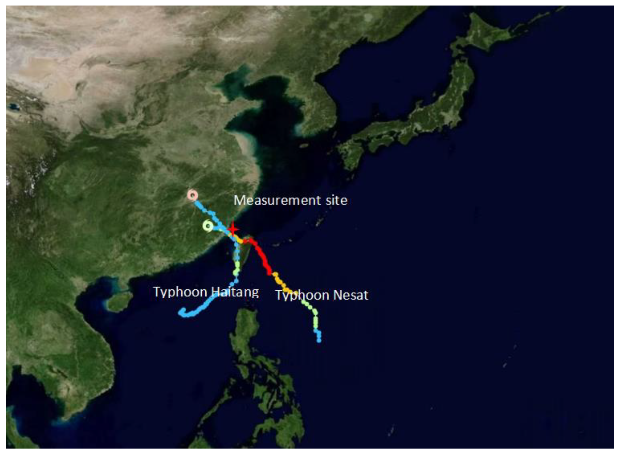
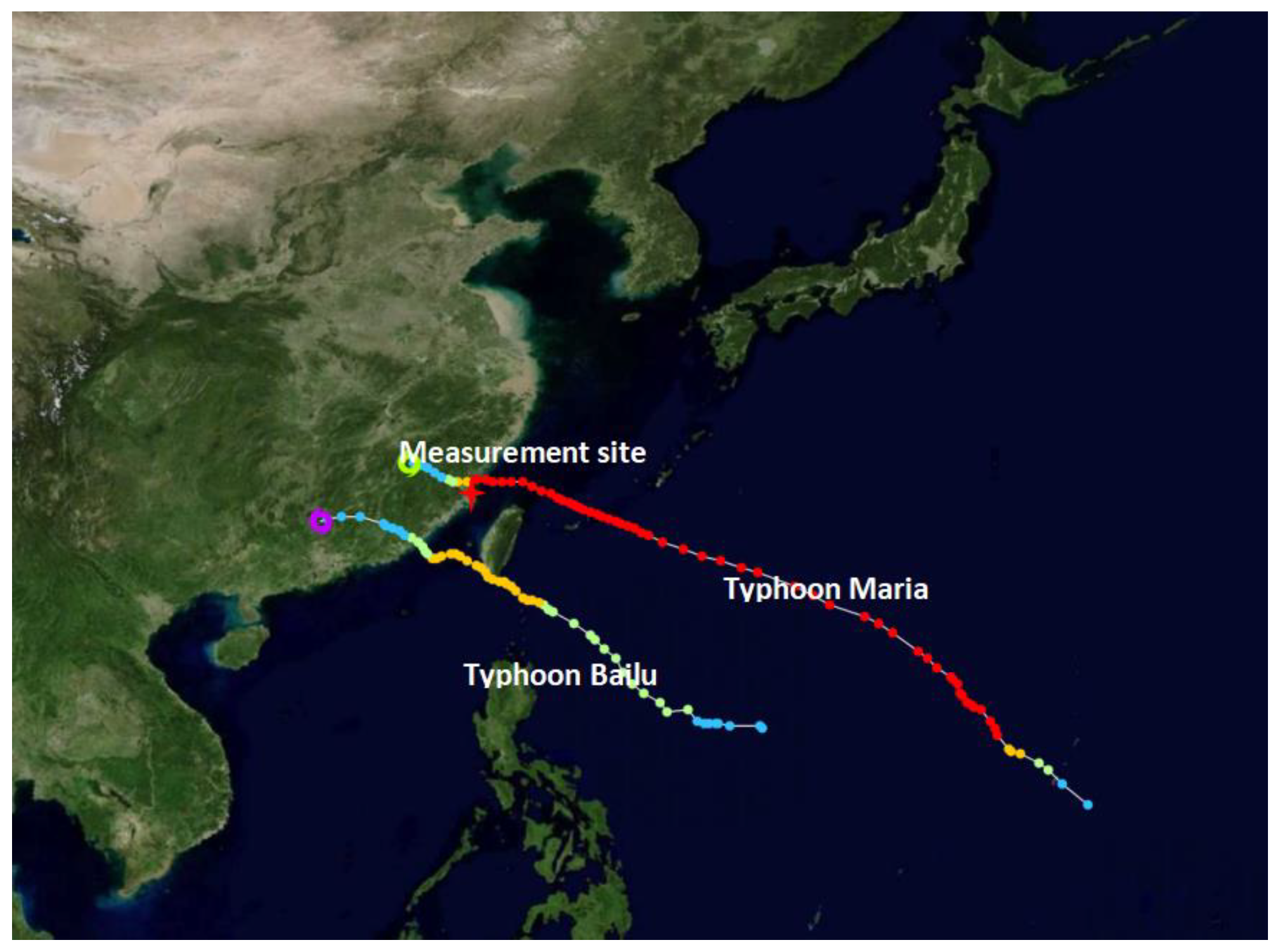
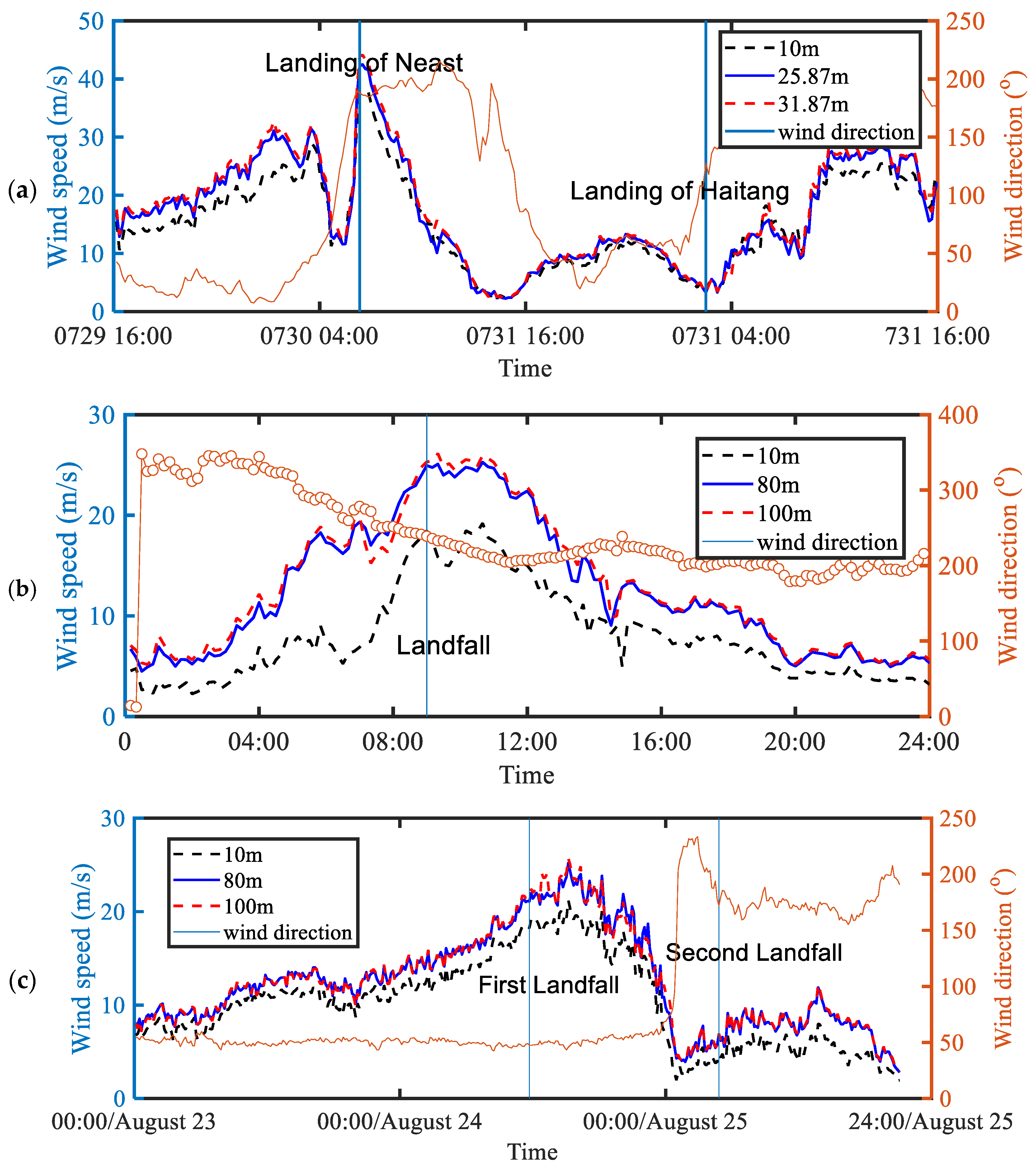
• Based on the measured data and data control method, the wind speeds of the four typhoon processes Nesat, Haitang, Maria, and Bailu were obtained for fractal analysis.
• In the box-counting method, the fractal dimensions generally vary between 1.3 and 1.5. The fractal dimensions differ with different measurement sites due to the influence of terrain conditions. The fractal dimensions slightly vary with measurement height. The maximum fractal dimension values occur when a typhoon makes landfall, indicating the complexity of wind speeds during typhoon landfall.
• Multifractality can be found in typhoon wind speeds as the fractal dimensions change with scale by multifractal detrended fluctuation analysis. When selecting the physical parameters of a typhoon simulation model, it is vital to consider multi-fractality.
• In the MFDFA, the fractal parameters are generally greater than those that are determined by monofractal analysis, with Hurst exponents greater than 0.5 indicating that the original wind speed series are persistent.
• Fractal analysis is vital for explaining the inner dynamic nature of turbulence. This research can provide a reference for future typhoon predictions, such as typhoon simulations and the development of predictive models.

This research mainly focused on explaining the complexity of typhoon structures based on wind speed data. However, typhoon structures may be affected by various aspects such as temperature and pressure. To understand the dynamic characteristics of typhoons, we may need combine temperature and pressure data in future work.

References

1. Song, L.; Chen, W.; Wang, B.; Zhi, S.; Liu, A. Characteristics of wind profiles in the landfalling typhoon boundary layer. J. Wind Eng. Ind. Aerodyn. 2016, 149, 77–88. [Google Scholar]
2. Lin, L.; Chen, K.; Xia, D.; Wang, H.; Hu, H.; He, F. Analysis on the wind characteristics under typhoon climate at the southeast coast of China. J. Wind Eng. Ind. Aerodyn. 2018, 182, 37–48. [Google Scholar]
3. Xia, D.; Dai, L.; Lin, L.; Wang, H.; Hu, H. A Field Measurement Based Wind Characteristics Analysis of a Typhoon in Near-Ground Boundary Layer. Atmosphere 2021, 12, 873. [Google Scholar] [CrossRef]
4. Li, J.; Wang, H.; Wang, H. Numerical Simulation Analysis of Typhoon Moving Track on Sea Surface Cooling. J. Phys. Conf. Ser. 2024, 2718, 012002. [Google Scholar]
5. Pang, S.; Li, J.; Guo, T.; Ma, X. Influence of the Species Number of Hydrometeors on Numerical Simulation of the Super Typhoon Mujigae in 2015. Asia-Pac. J. Atmos. Sci. 2023, 60, 29–47. [Google Scholar]
6. Tao, T.Y.; Wang, H.; Wu, T. Stationary and non-stationary analysis on the wind characteristics of a tropical storm. Smart Struct. Syst. 2016, 17, 1067–1085. [Google Scholar]
7. He, X.; Qin, H.; Tao, T.; Liu, W.; Wang, H. Measurement of Non-Stationary Characteristics of a Landfall Typhoon at the Jiangyin Bridge Site. Sensors 2017, 17, 2186. [Google Scholar] [CrossRef]
8. Fang, G.S.; Zhao, L.; Cao, S.Y.; Ge, Y.J.; Pang, W.C. A novel analytical model for wind field simulation under typhoon boundary layer considering multi-field correlation and height-dependency. J. Wind. Eng. Ind. Aerod. 2018, 175, 77–89. [Google Scholar]
9. Jin, J.; Wang, B.; Yu, M.; Liu, J.; Wang, W. A Novel Self-Adaptive Wind Speed Prediction Model Considering Atmospheric Motion and Fractal Feature. IEEE Access 2020, 8, 215892–215903. [Google Scholar]
10. Breslin, M.; Belward, J. Fractal dimensions for rainfall time series. Math. Comput. Simulat. 1999, 48, 437–446. [Google Scholar]
11. Ribeiro, M.B.; Miguelote, A.Y. Fractals and the distribution of galaxies. Braz. J. Phys. 1998, 28, 132–160. [Google Scholar] [CrossRef]
12. Falconer, K. Fractal Geometry: Mathematical Foundations and Applications; John Wiley & Sons: Hoboken, NJ, USA, 2004. [Google Scholar]
13. Kavasseri, R.G.; Nagarajan, R. A multifractal description of wind speed records. Chaos Solitons Fractals 2005, 24, 165–173. [Google Scholar] [CrossRef]
14. Feng, T.; Fu, Z.; Deng, X.; Mao, J. A brief description to different multi-fractal behaviors of daily wind speed records over China. Phys. Lett. A 2009, 45, 4134–4141. [Google Scholar] [CrossRef]
15. Chang, T.; Ko, H.-H.; Liu, F.; Chen, P.; Chang, Y.; Liang, Y.-H.; Jang, H.-Y.; Lin, T.-C.; Chen, Y.-H. Fractal dimension of wind speed time series. Appl. Energy 2012, 93, 742–749. [Google Scholar] [CrossRef]
16. Fortuna, L.; Nunnari, S.; Guariso, G. Fractal order evidences in wind speed time series. In Proceedings of the ICFDA’14 International Conference on Fractional Differentiation and Its Applications, Catania, Italy, 23–25 June 2014; IEEE: Piscataway, NJ, USA, 2014; pp. 1–6. [Google Scholar]
17. Laib, M.; Golay, J.; Telesca, L.; Kanevski, M. Multifractal analysis of the time series of daily means of wind speed in complex regions. Chaos Solitons Fractals 2018, 109, 118–127. [Google Scholar] [CrossRef]
18. Balkissoon, S.; Fox, N. Anthony LupoFractal characteristics of tall tower wind speeds in Missouri. Renew. Energy 2020, 154, 1346–1356. [Google Scholar] [CrossRef]
19. Cui, B.; Huang, P.; Xie, W. Fractal dimension characteristics of wind speed time series under typhoon climate. J. Wind. Eng. Ind. Aerodyn. 2022, 229, 105144. [Google Scholar] [CrossRef]
20. Liang, J.; Li, L.; Chan, P.W.; Zhang, L.; Lu, C. Honglong Yang, Fractal dimension characterization of wind speed in typhoons and severe convective weather events based on box dimension analysis. Chaos Solitons Fractals 2024, 186, 115301. [Google Scholar] [CrossRef]
21. Shu, Z.R.; Chan, P.W.; Li, Q.S.; He, Y.C.; Yan, B.W. Quantitative assessment of offshore wind speed variability using fractal analysis. Wind. Struct. 2020, 31, 363–371. [Google Scholar]
22. Malinverno, A. A simple method to estimate the fractal dimension of a self-affine series. Geophys. Res. Lett. 1990, 17, 1953–1956. [Google Scholar] [CrossRef]
23. Burrough, P.A. Fractal dimensions of landscapes and other environmental data. Nature 1981, 294, 240–242. [Google Scholar] [CrossRef]
24. Espen, A.F. Ihlen Multifractal analyses of response time series: A comparative study. Behav. Res. Methods 2013, 45, 928–945. [Google Scholar]
25. Gu, G.; Zhou, W. Detrending moving average algorithm for multifractals. Phys. Rev. E 2010, 82, 011136. [Google Scholar] [CrossRef]
26. Zhao, G.; Deng, Q.; Li, X.; Dong, L.; Chen, G.; Zhang, C. Recognition of microseismic waveforms based on EMD and morphological fractal dimension. J. Cent. South Univ. (Sci. Technol.) 2017, 48, 162–167. [Google Scholar]
27. Cadenas, E.; Campos-Amezcua, R.; Rivera, W.; Espinosa-Medina, M.A.; Mendez-Gordillo, A.R.; Rangel, E.; Tena, J. Wind speed variability study based on the Hurst coefficient and fractal dimensional analysis. Energy Sci. Eng. 2019, 7, 361–378. [Google Scholar] [CrossRef]
28. Harrouni, S.; Guessoum, A. Using fractal dimension to quantify long-range persistence in global solar radiation. Chaos Soliton Fract 2009, 41, 1520–1530. [Google Scholar] [CrossRef]
29. de Figueiredo, B.C.L.; Moreira, G.R.; Stosic, B.; Stosic, T. Multifractal analysis of hourly wind speed records in petrolina, northeast Brazil. Rev. Bras. Biom. 2014, 32, 599–608. [Google Scholar]
30. Kantelhardt, J.W.; Zschiegner, S.A.; Koscielny-Bunde, E.; Havlin, S.; Bunde, A.; Stanley, H.E. Multifractal detrended fluctuation analysis of nonstationary time series. Phys. Stat. Mech. Appl. 2002, 316, 87–114. [Google Scholar] [CrossRef]
31. Movahed, M.S.; Jafari, G.; Ghasemi, F.; Rahvar, S.; Tabar, M.R.R. Multifractal detrended fluctuation analysis of sunspot time series. J. Stat. Mech. Theor. Exp. 2006, 2006, P02003. [Google Scholar] [CrossRef]
Figure 1. Locations of the measurement sites.
Fractalfract 09 00175 g001
Figure 2. Wind measurement tower and anemometers for the WM Station.
Fractalfract 09 00175 g002
Figure 3. Wind measurement tower and anemometers for the YI Station [3].
Fractalfract 09 00175 g003
Figure 4. Landfall Events of Typhoons Nesat and Haitang.
Fractalfract 09 00175 g004
Figure 5. Landfall Events of Typhoons Maria and Bailu.
Fractalfract 09 00175 g005
Figure 6. Wind speeds and wind directions of Typhoons (a) Nesat and Haitang, (b) Maria, and (c) Bailu.
Fractalfract 09 00175 g006
Figure 7. Log–log diagrams of the fractal dimensions for using 10-min wind speed time series for Typhoons (a) Nesat, (b) Haitang, (c) Maria, and (d) Bailu.
Fractalfract 09 00175 g007
Figure 8. The time series of the 10-min fractal dimensions for Typhoons (a) Nesat and Haitang, (b) Maria, and (c) Bailu.
Fractalfract 09 00175 g008
Figure 9. Flow chart of MFDFA analysis process.
Fractalfract 09 00175 g009
Figure 10. Time history of the recorded wind speeds (10 min).
Fractalfract 09 00175 g010
Figure 11. The MFDFA results of the wind speed time series obtained from the measuring station: (a) Fluctuation functions for q = −5, q = 0, and q = 5. (b) Generalized Hurst exponents for each q value. (c) τ (q) function. (d) Multifractal spectrum.
Fractalfract 09 00175 g011
Figure 12. Scaling function F(q) vs. q based on typhoon wind speeds (a) Nesat, (b) Haitang, (c) Maria, and (d) Bailu.
Fractalfract 09 00175 g012
Figure 13. Generalized Hurst Exponents based on typhoon wind speeds (a) Nesat, (b) Haitang, (c) Maria, and (d) Bailu.
Fractalfract 09 00175 g013
Figure 14. Mass exponents based on typhoon wind speeds (a) Nesat, (b) Haitang, (c) Maria, and (d) Bailu.
Fractalfract 09 00175 g014
Figure 15. Multifractal spectra based on typhoon wind speeds (a) Nesat, (b) Haitang, (c) Maria, and (d) Bailu.
Fractalfract 09 00175 g015aFractalfract 09 00175 g015b
Figure 16. Spectral widths and Hurst exponents based on wind speeds in Typhoon (a) Nesat and Haitang, (b) Maria, and (c) Bailu.
Fractalfract 09 00175 g016aFractalfract 09 00175 g016b
Figure 17. Histograms of the Hurst exponents for different typhoons; (a) Nesat and Haitang, (b) Maria, and (c) Bailu.
Fractalfract 09 00175 g017