Revisiting the Consolidation Model by Taking the Rheological Characteristic and Abnormal Diffusion Process into Account

Abstract

With the increasing construction of engineering structures on soft soils, accurately assessing their consolidation behavior has become crucial. To address this, Terzaghi’s one-dimensional consolidation model was revisited. The elastic behavior of soil skeleton was modified by incorporating viscous effects using the fractional derivative Merchant model (FDMM), while the linear Darcy’s law governing flux–pressure relations was extended by introducing time memory formalism through the fractional derivative Darcy model (FDDM). The governing equation is derived by incorporating the resulting constitutive behavior of both the soil skeleton and water flow into the Terzaghi’s formulation of the poroelasticity problem. The proposed rheological consolidation model is solved by a forward time-centered space scheme (FTCS). After verifying the numerical procedure with published data, the influence of parameters on both the average degree of settlement and the pressure was comprehensively studied.

1. Introduction

The long-term safety and functionality of geotechnical structures on soft clay, such as high-rise buildings, long-span bridges, maritime infrastructure, and underground works, have always been a major concern. Although the research on soft clay has a long history, it was not until Terzaghi proposed the linear elastic consolidation theory that a solid theoretical foundation was established [1]. Since then, numerous mathematical models have been introduced to describe the typical phenomena occurring during the consolidation process.

Soft soils are characterized by fine particles, high water content, high compressibility, low permeability, and unique structural characteristics. These properties make soft soil behavior distinct from other soils under long-term sustained loads. For one aspect, the fine particles in soft soils are surrounded by water a film that inhibits interparticle sliding due to frictional and adhesive forces, resulting in a time-dependent response [2]. For another aspect, particle rearrangement and subsequent compaction lead to a reduction of permeability, which introduces non-linearity into the diffusion process and accordingly, complicates the analytical solutions to the governing equations.

To address the discrepancies between experimentally observed behavior and model predictions, various models have been developed. The rheological behavior of soft soil skeletons has primarily been characterized by component models, such as the Maxwell model [3], the Kelvin–Voigt model [4,5], and the Merchant model [6,7]. They were designed to fit the creep or relaxation curve by combining the features of Hooke’s elastomer and Newtonian viscous body. Due to their adaptability and effectiveness, as well as feasible implementation in commercial software, component models have been widely used in early research. However, accurately representing complex viscoelastic behavior often requires many elements (Hooke’s elastomer and Newtonian viscous body), which complicates parameter calibration and sometimes results in overfitting of experimental data, particularly the initial stages of creep compliance and relaxation moduli. This motivates the search for a simplified constitutive model. The fractional calculus could be the solution.

Fractional calculus extends traditional integer order derivative to real one, typically between 0 and 1. By adjusting the order, the fractional model allows smoothly transitions between elastic (order 0) and viscous (order 1) behavior. This inherent property makes the fractional calculus an excellent tool for modeling memory-intensive and path-dependent phenomena. Moreover, by replacing integer-order Newtonian elements with fractional derivatives, such as Captuo [8], Riemann–Liouville [9], Caputo–Fabrizio [10], the consolidation behavior of single soil layer under cyclic loading [11] or multilayered under time-dependent loading [12] could be more accurately described.

In Terzaghi’s one-dimensional consolidation theory, the flow behavior of water fluid through the homogeneous isotropic soil layer satisfies linear Darcy’s law, namely the volumetric flux is linearly related to the pressure gradient. However, long-term consolidation may result in time-varying permeability in saturated soils due to chemical reactions between fluids and porous mediums [13], migration of solid particles due to fluid flow [14], and soil compaction [15,16]. These facts indicate that the traditional linear Darcy’s law may be inadequate in certain cases. To address this, researchers have sought to modify or extend Darcy’s law by incorporating factors, such as inertia [17,18] and slip [19]. Fractional calculus, with its intrinsic properties, provides an alternative framework to account for non-linear diffusion processes. To date, the fractional derivative-based Darcy’s law has three types of form: (1) fractional derivatives to capture pressure variation [20]; (2) Caputo fractional derivatives to modify permeability [21]; (3) fractional derivatives applied to space pressure variation [22].

An inappropriate fractional derivative-based seepage model will not only complicate experimental data fitting but also challenge the reasonable interpretation of water flow behavior. For instance, during a long-term constant head test, the pressure gradient at any instant is not measurable. Therefore, it is usually assumed that it is a constant to facilitate the calculation. However, in a Caputo fractional derivative-based seepage model, experimental data fitting requires an additional empirical formula, as the derivative of a constant is zero.

This study proposes an alternative form of fractional derivative (RL fractional derivative) that is used to modify Caputo’s fractional derivative-based Darcy model. The RL fractional derivative of a constant results in a time-dependent power function facilitating experimental data fitting. After demonstrating the effectiveness of the proposed model, it is combined with the fractional derivative-based Merchant model to form a one-dimensional rheological consolidation model. The nonlinear consolidation characteristics of soft soils under ramp loading [23,24] are qualitatively analyzed and discussed.

2. Fractional Derivative-Based Model

2.1. Basics of Fractional Calculus

Let a function $f\left(t\right)$ be continuous on $\left[a,b\right]$, the widely used upper form of its RL fractional integral of order $\beta >0$ is defined as follows [25]:

$${}_{a}I_t^{\beta }f(t)={\displaystyle \frac{1}{\Gamma (\beta )}}{\displaystyle {\int }_a^t{\left(t-\tau \right)}^{\beta -1}f(\tau )d\tau }$$

(1)

where $\Gamma \left(·\right)$ is the Euler gamma function.

Based on the definition of the RL fractional integral, the RL and Caputo fractional derivatives of order $\beta$ can be, respectively, defined as follows:

$${}_a{}^{\mathit{RL}}D_t^{\beta }f\left(t\right)={\displaystyle \frac{{\mathrm{d}}^m}{\mathrm{d}{t}^m}}{}_{a}I_t^{m-\beta }f(t)={\displaystyle \frac{1}{\Gamma (m-\beta )}}{\displaystyle \frac{{\mathrm{d}}^m}{\mathrm{d}{t}^m}}{{\displaystyle \int }}_a^t{\left(t-\tau \right)}^{m-\beta -1}f(\tau )d\tau$$

(2)

$${}_a{}^{C}D_t^{\beta }f(t)={}_{a}I_t^{m-\beta }{\displaystyle \frac{{\mathrm{d}}^m}{\mathrm{d}{t}^m}}f(t)={\displaystyle \frac{1}{\Gamma (m-\beta )}}{{\displaystyle \int }}_a^t{\left(t-\tau \right)}^{m-\beta -1}{f}^{\left(m\right)}(\tau )d\tau$$

(3)

The superscripts RL and C denote Riemann–Liouville and Caputo derivatives, respectively. $m$ is the smallest positive integer greater than $\beta$. Given that $\beta \in \left(0,1\right)$ is assumed in this paper, $m$ is set to 1.

By introducing a power function kernel, we obtain the following:

$$Y_{\beta }\left(t\right)={\displaystyle \frac{t_{+}^{\beta -1}}{\Gamma \left(\beta \right)}}$$

(4)

where $t_{+}^{\beta -1}=0$ if $t\le 0$, while $t_{+}^{\beta -1}=t^{\beta -1}$ if $t>0$. The fractional derivatives mentioned can be rewritten according to the convolution theorem, written as follows:

$${}_a{}^{\mathit{RL}}D_t^{\beta }f\left(t\right)={\displaystyle \frac{{\mathrm{d}}^m}{\mathrm{d}{t}^m}}\left(Y_{m-\beta }\left(t\right)\ast f(t)\right)={\displaystyle \frac{1}{\Gamma (m-\beta )}}{\displaystyle \frac{{\mathrm{d}}^m}{\mathrm{d}{t}^m}}{{\displaystyle \int }}_a^t{\left(t-\tau \right)}^{m-\beta -1}f(\tau )\mathrm{d}\tau$$

(5)

$${}_a{}^{C}D_t^{\beta }f(t)=Y_{m-\beta }\left(t\right)\ast \left({\displaystyle \frac{{\mathrm{d}}^m}{\mathrm{d}{t}^m}}f(t)\right)={\displaystyle \frac{1}{\Gamma (m-\beta )}}{{\displaystyle \int }}_a^t{\left(t-\tau \right)}^{m-\beta -1}{f}^{\left(m\right)}(\tau )\mathrm{d}\tau$$

(6)

It is important to note that the output of a fractional derivative can be understood as a weighted sum of all previous input values $f(\tau )$ multiplied by the impulse response ${\left(t-\tau \right)}^{m-\beta -1}$. This implies that the value of the fractional derivative depends not only on the present value but also on its entire history. This capacity for accounting for long-term memory makes the fractional derivative particularly useful in modeling viscoelasticity and anomalous diffusion.

2.2. Fractional Derivative Merchant Model

Under long-term sustained loads, the skeleton of soft soils undergoes time-dependent deformation that integrates both elastic and viscous characteristics. To describe these mechanical behaviors, the component models, which combine features of Hooke’s elastomer and Newtonian viscous body, are commonly employed in classical viscoelasticity. The widely used Merchant model, as shown in Figure 1a, consists of a Hooke’s elastomer with elastic modulus $E_0$ and a Kelvin element in series, and each Kelvin model is made up of a Newtonian viscous body with viscosity coefficient $F$ in parallel with a Hooke’s elastomer with elastic modulus $E_1$.

For a Merchant material, the effective stress ${\sigma }^{\prime }$ and strain $\epsilon$ supported by the skeleton of soft soils, along with their time derivatives, are governed by the following equation:

$${\sigma }^{\prime }+{\displaystyle \frac{F}{E_0+E_1}}{\displaystyle \frac{\partial {\sigma }^{\prime }}{\partial t}}={\displaystyle \frac{E_0{E}_1}{E_0+E_1}}\epsilon +{\displaystyle \frac{F{E}_0}{E_0+E_1}}{\displaystyle \frac{\partial \epsilon }{\partial t}}$$

(7)

To more accurately capture the time-dependent characteristics of soft soil skeleton, Koeller proposed replacing the classical Newtonian viscous body with a fractional derivative one known as spring-pot, whose constitutive law satisfies the following [26]:

$${\sigma }_{\eta }=E{\eta }^{\alpha }{}_0{}^{C}D_{\mathrm{t}}^{\alpha }\epsilon$$

(8)

where $\eta =F/E$ is named as either the relaxation time or viscosity time, depending on the specific model being analyzed. ${}_0{}^{C}D_{\mathrm{t}}^{\alpha }\left(•\right)$ is the Caputo fractional derivative operator defined in Equation (3).

Just as its name indicates, the spring-pot could mimic the behavior of spring (Hooke’s elastomer) when $\alpha \to 0$ or pot (Newtonian viscous body) when $\alpha \to 1$. As the spring element has no memory and the pot element has perfect memory, the material described by the spring-pot with value of $\alpha$ between 0 and 1 exhibits memory to some extent. Replacing the Newtonian viscous element in the conventional Merchant model with a spring-pot element yields the fractional derivative-based Merchant model (FDMM), whose behavior is governed by the following:

$$\sigma +{\displaystyle \frac{E_1{\eta }^{\alpha }}{E_0+E_1}}{}_0{}^{C}D_{\mathrm{t}}^{\alpha }\sigma ={\displaystyle \frac{E_0{E}_1}{E_0+E_1}}\epsilon +{\displaystyle \frac{E_0{E}_1{\eta }^{\alpha }}{E_0+E_1}}{}_0{}^{C}D_{\mathrm{t}}^{\alpha }\epsilon$$

(9)

It is notable that dimensional homogeneity in Equations (8) and (9) the is ensured by the parameter ${\eta }^{\alpha }$.

Under the assumption of infinitesimal strain, the constitutive equation relating strain $\epsilon$ to effective stress ${\sigma }^{\prime }$ is given by the form of a hereditary integral as follows:

$$\epsilon (t)={\displaystyle {\int }_0^{t}J(t-\tau )\mathrm{d}{\sigma }^{\prime }(\tau )}={\displaystyle {\int }_0^{t}J(t-\tau )\frac{\partial {\sigma }^{\prime }(\tau )}{\partial \tau }\mathrm{d}\tau }$$

(10)

$$J(t)={\displaystyle \frac{1}{E_0}}+{\displaystyle \frac{1}{E_1}}\left\{1-E_{\alpha }\left[-{\left({\displaystyle \frac{t}{\eta }}\right)}^{\alpha }\right]\right\}$$

(11)

where $J\left(t\right)$ is the creep compliance $E_{\alpha }(x)={\displaystyle {\sum }_{k=0}^{\infty }{x}^k/\Gamma \left(\alpha k+1\right)}$. is Mittag–Leffler function.

The effect of the fractional order $\alpha$ on creep behavior is illustrated in Figure 2. The parameters adopted are: ${\sigma }^{\prime }=20 \mathrm{kPa}$, $E_0=20 \mathrm{MPa}$, $E_1=20 \mathrm{MPa}$, and $\eta =30 \mathrm{s}$. It is found that creep strain increases with the fractional order $\alpha$, showing the dependence of creep strain on the fractional order.

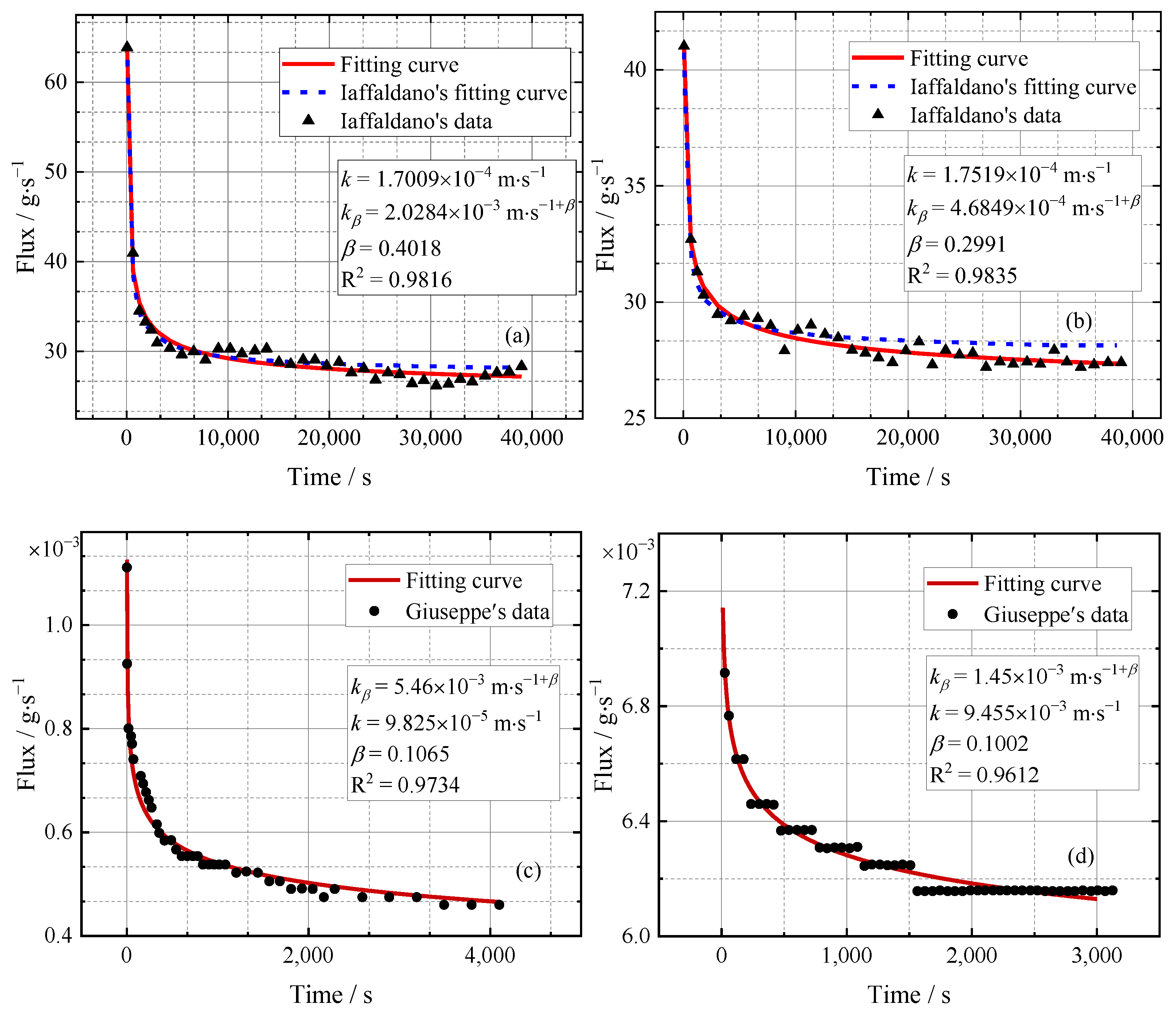
2.3. Fractional Derivative-Based Darcy Model

In Terzaghi’s one-dimensional consolidation theory, the flow of water through the homogeneous isotropic soil layer is governed by Darcy’s law, which states that the volumetric flux $q$ is linearly related to the pressure gradient $\nabla u$, written as follows:

$$q=-{\displaystyle \frac{k}{{\gamma }_{\mathrm{f}}}}\nabla u$$

(12)

where $k$ is permeability coefficient and ${\gamma }_{\mathrm{f}}$ represents the unit weight of water.

In long-term water flow, the compaction of soil skeleton leads to a decrease in permeability. At any instant, the diffusion process is affected by the history of pressure, which indicates water flow behavior, a non-local characteristic. To account for this anomalous diffusion process, the linear form of Darcy’s law is modified by incorporating a memory formalism. Inspired by the work of Alaimo [27], the pressure-flux relationship now changes to:

$${\gamma }_{\mathrm{f}}q=-(k+k_{\beta }{}_0{}^{\mathit{RL}}D_{\mathrm{t}}^{\beta })\nabla u$$

(13)

where ${}_0{}^{\mathit{RL}}D_{\mathrm{t}}^{\beta }\left(•\right)$ the RL fractional derivative as defined in Equation (2) and $k_{\beta }$ denotes the anomalous permeability coefficient, which has a unit of $\mathrm{m}/{\mathrm{s}}^{1-\beta }$. This is distinct from the unit of classical permeability due to the incorporation of the fractional derivative. Physically, $k_{\beta }$ describes the medium’s ability to facilitate fluid flow, considering the memory effect introduced by the fractional model.

The effectiveness of the fractional derivative-based Darcy model (FDDM) is checked by fitting the predictions to the oedometer test results. Figure 3 shows the comparisons between the model presented in this paper and the data from Iaffaldano et al. [28] and Giuseppe et al. [21]. In general, the flow behavior of water through soil could be well described.

3. One-Dimension Consolidation Model of Rheological Soils

3.1. Governing Equations, Boundary Conditions and Initial Conditions

The schematic diagram of a 1D rheological consolidation model is depicted in Figure 4. The total thickness of the soil layer is $h$. The top surface is pervious and free, whereas the bottom one is impervious and fixed. The top surface is subjected to a uniform time-dependent load $p\left(t\right)$.

The derivation of the 1D rheological consolidation model follows Terzaghi’s work except for the following:

(1)

Deformation of the soil skeleton is governed by FDMM;

(2)

Water flow through an isotropic homogeneous layer is governed by FDDM.

Under the assumption of constant water density, the fluid mass balance relation requires the variation of fluid volume per unit volume of a soil unit equals the volumetric discharge of water out of that unit, namely as follows:

$${\displaystyle \frac{\partial \epsilon }{\partial t}}=-{\displaystyle \frac{\partial q}{\partial x}}$$

(14)

It is worth pointing out that the expansion of the soil unit indicates a “gain” of fluid content.

Substituting Equations (10) and (13) into Equation (14) yields the governing equation of 1D rheological consolidation model:

$${\displaystyle \frac{\partial {\displaystyle {\int }_0^{t}J(t-\tau )\frac{\partial (u-p)}{\partial \tau }\mathrm{d}\tau }}{\partial t}}=\left(c+c_{\beta }{}_0{}^{\mathit{RL}}D_{\mathrm{t}}^{\beta }\right){\nabla }^{2}u$$

(15)

where $c=k/{\gamma }_{\mathrm{f}}$ and $c_{\beta }=k_{\beta }/{\gamma }_{\mathrm{f}}$.

The initial and boundary conditions are as follows:

$$u(x,0)=u_0\left\{\begin{array}{c}u\left(h,t\right)=0\\ {\displaystyle \frac{\partial u\left(0,t\right)}{\partial x}}=0\end{array}\right.$$

(16)

3.2. Time-Dependent Load

In practical engineering, the consolidation stress, such as preloading and vacuum preloading, is applied gradually and incrementally over time rather than instantaneously, as illustrated in Figure 5. This type of loading is referred to as multi-stage ramp loading.

Let the entire loading process be discretized as $\left[0,T\right]={\cup }_{n=1}^N\left[t_{2n-2},t_{2n}\right]$. Within any typical time interval, $\left[t_{2n-2},t_{2n}\right]$, the consolidation stress is applied at a steady rate over the time interval, $\left[t_{2n-2},t_{2n-1}\right]$, from the value at the end of the previous step to the targeted value, and then maintains a constant over the time interval, $\left[t_{2n-1},t_{2n}\right]$. Under this definition, the loading function can be written as follows:

$$p\left(t\right)=\left\{\begin{array}{cc}\hfill p_{n-1}+{\displaystyle \frac{t-t_{2n-2}}{t_{2n-1}-t_{2n-2}}}\left(p_n-p_{n-1}\right)& t_{2n-2}\le t\le t_{2n-1}\hfill \\ p_n& t_{2n-1}\le t\le t_{2n} \hfill \end{array}\right.$$

(17)

4. Numerical Solution to the 1D Rheological Consolidation Model

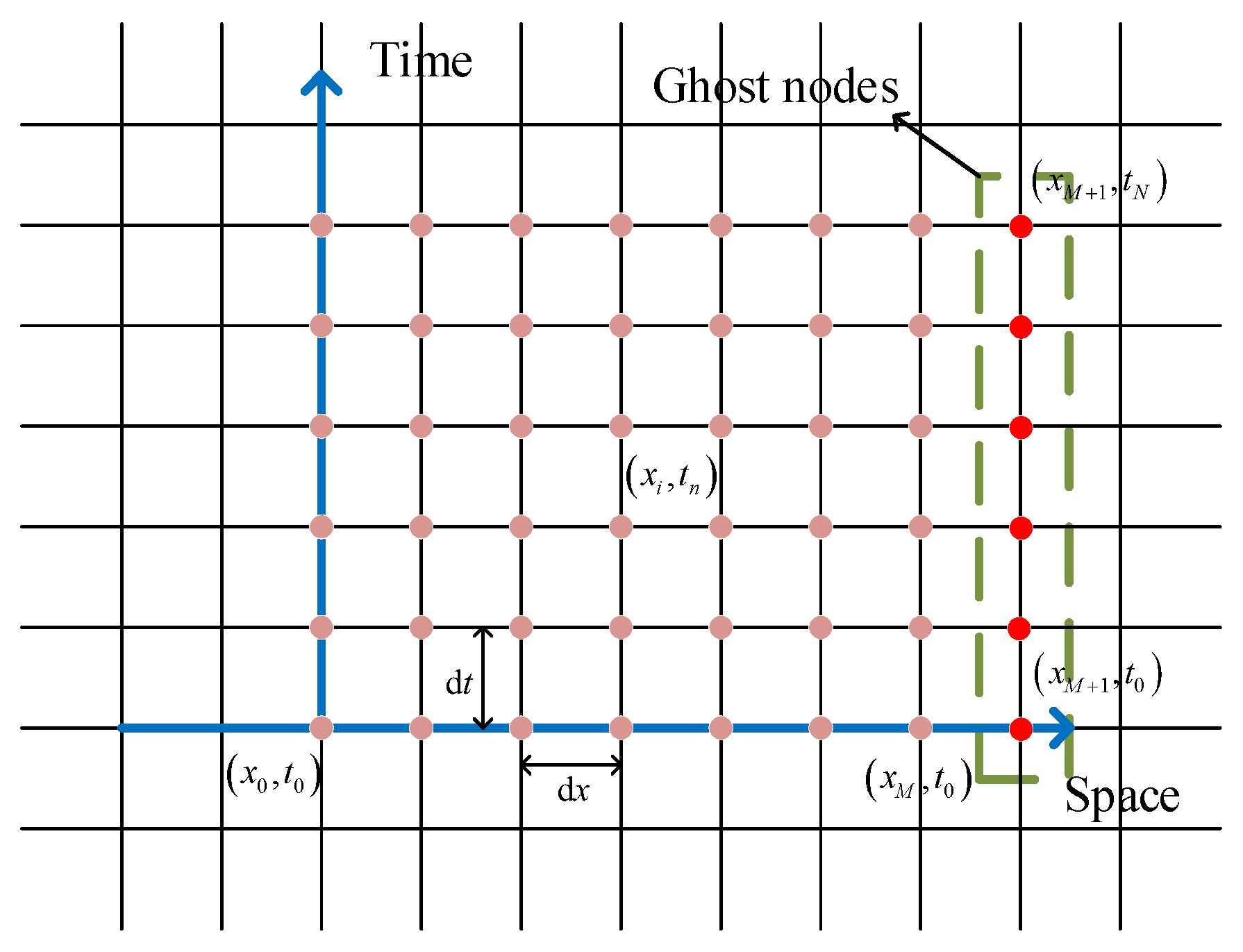
4.1. Forward Time-Centered Space Scheme

The proposed 1D rheological consolidation model is solved by a forward time-centered space scheme (FTCS). To facilitate the subsequent validation, Equation (15) is first recast into the following:

$$\begin{array}{r}\hfill {\displaystyle \frac{\partial {\displaystyle {\int }_0^{t}J(t-\tau )\frac{\partial (u-p)}{\partial \tau }d\tau }}{\partial t}}=c{\displaystyle \frac{{\partial }^{2}u(x,t)}{\partial x^2}}+\left[c_{\beta }{\mathcal{D}}_{0,t}^{1-r}\left({\displaystyle \frac{{\partial }^{2}u(x,t)}{\partial x^2}}\right)\right]+f(x,t)\\ \hfill 0<x<L,\hspace{1em}0<t\le T.\end{array}$$

(18)

$$\left\{\begin{array}{c}u\left(0,t\right)=0\\ {\displaystyle \frac{\partial u\left(L,t\right)}{\partial x}}=0\end{array}\right.u(x,0)=u_0$$

(19)

where $\beta =1-r$ and $f\left(x,t\right)$ can be considered as a source term.

To derive the finite difference format of Equation (18), a grid of points needs to be firstly defined in the $\left(x,t\right)$ plane. Let $M$ and $N$ be two positive integers defining the number of equally spaced points in the spatial and temporal domains, respectively. The intervals of length in the spatial and temporal directions are represented by $\mathrm{d}x=L/M$ and $\mathrm{d}t=T/N$, as shown in Figure 6. With this definition, $x_i=i\mathrm{d}x$($0\le i\le M$) and $t_n=n\mathrm{d}t$($0\le n\le N$).

To simplify the subsequent derivation, the following operators need to be firstly defined as follows:

$$\begin{array}{l}{\delta }_x{}^{2}u_i^n={\displaystyle \frac{1}{\mathrm{d}{x}^2}}(u_{i-1}^n-2u_i^n+u_{i+1}^n)\\ {\delta }_t{u}_i^{n-{\displaystyle \frac{1}{2}}}={\displaystyle \frac{1}{\mathrm{d}t}}(u_i^n-u_i^{n-1})\\ {\delta }_x^2{u}_i^{n-{\displaystyle \frac{1}{2}}}={\displaystyle \frac{1}{2}}({\delta }_x{}^{2}u_i^n+{\delta }_x{}^{2}u_i^{n-1})\end{array}$$

(20)

Following the FTCS scheme, the forward difference is applied to approximate the first-order time derivative at a given point, namely as follows:

$$\begin{array}{ll}\hfill {\displaystyle \frac{\partial {\int }_0^{t}J(t-\tau )\frac{\partial (u-p)}{\partial \tau }\mathrm{d}\tau }{\partial t}}& ={\displaystyle \frac{1}{\mathrm{d}t}}\left[{\displaystyle {\int }_0^{t_n}J(t_n-\tau )\frac{\partial (u-p)}{\partial \tau }\mathrm{d}\tau }-{\displaystyle {\int }_0^{t_{n-1}}J(t_{n-1}-\tau )\frac{\partial (u-p)}{\partial \tau }\mathrm{d}\tau }\right]\hfill \\ \hfill & ={\displaystyle \frac{1}{\mathrm{d}t}}\left\{{\displaystyle {\int }_0^{t_{n-1}}\left[J(t_n-\tau )-J(t_{n-1}-\tau )\right]\frac{\partial (u-p)}{\partial t}\mathrm{d}\tau }+{\displaystyle {\int }_{t_{n-1}}^{t_n}J(t_n-\tau )\frac{\partial (u-p)}{\partial \tau }\mathrm{d}\tau }\right\}\hfill \\ & ={\displaystyle \frac{1}{\mathrm{d}t}}\left\{\begin{array}{l}\left(u^n-p^n-u^{n-1}+p^{n-1}\right)/\mathrm{d}t\cdot J\left(t_n-{\displaystyle \frac{t_n+t_{n-1}}{2}}\right)\cdot \mathrm{d}t+\\ {\displaystyle {\displaystyle \sum }_{k=1}^{n-1}}\left(u^k-p^k-u^{k-1}+p^{k-1}\right)\left[J\left(t_n-{\displaystyle \frac{t_k+t_{k-1}}{2}}\right)-J\left(t_{n-1}-{\displaystyle \frac{t_k+t_{k-1}}{2}}\right)\right]\end{array}\right\}\hfill \\ & ={\displaystyle \sum _{k=1}^{n-1}\left(J\left[\left(n-k+\frac{1}{2}\right)\mathrm{d}t\right]-J\left[\left(n-k-\frac{1}{2}\right)\mathrm{d}t\right]\right)}\left({\delta }_t{u}^{k-{\displaystyle \frac{1}{2}}}-{\delta }_t{p}^{k-{\displaystyle \frac{1}{2}}}\right)\hfill \\ & +J\left({\displaystyle \frac{\mathrm{d}t}{2}}\right)\left({\delta }_t{u}^{n-{\displaystyle \frac{1}{2}}}-{\delta }_t{p}^{n-{\displaystyle \frac{1}{2}}}\right)\hfill \end{array}$$

(21)

At a given time, the central difference is employed to approximate the second-order space derivative-based on the approximation of RL fractional derivative, written as follows [29]:

$$\left[D_{0,t}^{1-r}\left({\displaystyle \frac{{\partial }^2{u}_i^n}{\partial x^2}}\right)\right]={\displaystyle \frac{\mathrm{d}{t}^{r-1}}{\Gamma (1+r)}}\left[\begin{array}{l}-{\displaystyle {\displaystyle \sum }_{k=1}^{n-1}}(a_{n-k-1}-a_{n-k}){\delta }_x^2{u}_i^k\\ -a_{n-1}{\delta }_x^2{u}_i^0+{\delta }_x^2{u}_i^n\end{array}\right]+{\displaystyle \frac{t_n^{r-1}}{\Gamma (r)}}{\delta }_x^2{u}_i^0$$

(22)

To establish the finite difference format of Equation (18), $n=1$ and $n>1$ need to be separately taken into account due to the cumulative terms in Equations (21) and (22).

For $n=1$, we obtain the following:

$$\left({\delta }_t{u}_i^{{\displaystyle \frac{1}{2}}}-{\delta }_t{p}_i^{{\displaystyle \frac{1}{2}}}\right)J\left({\displaystyle \frac{\mathrm{d}t}{2}}\right)={\displaystyle \frac{c_{\beta }\mathrm{d}{t}^{r-1}}{\Gamma (r+1)}}\left[{\delta }_x{}^{2}u_i^1+\left(r-1\right){\delta }_x{}^{2}u_i^0\right]+c\cdot {\delta }_x{}^{2}u_i^{{\displaystyle \frac{1}{2}}}+f_i^1$$

(23)

Expanding Equation (23) yields the following:

$$\begin{array}{ll}\hfill J\left({\displaystyle \frac{\mathrm{d}t}{2}}\right)\left(u_i^1-u_i^0-p_i^1+p_i^0\right)=& s{u}_{i+1}^1-2s{u}_i^1+s{u}_{i-1}^1+s\left(r-1\right)\left(u_{i+1}^0-2u_i^0+u_{i-1}^0\right)\hfill \\ & +b{u}_{i+1}^1-2b{u}_i^1+b{u}_{i-1}^1+b{u}_{i+1}^0-2b{u}_i^0+b{u}_{i-1}^0+\mathrm{d}t{f}_i^1\end{array}$$

(24)

Rearranging Equation (24) yields the following:

$$\begin{array}{l}-\left(s+b\right)u_{i-1}^1+\left[J\left({\displaystyle \frac{\mathrm{d}t}{2}}\right)+2s+2b\right]u_i^1-\left(s+b\right)u_{i+1}^1\\ =\left(sr-s+b\right)u_{i-1}^0-2\left[sr-s-{\displaystyle \frac{1}{2}}J\left({\displaystyle \frac{\mathrm{d}t}{2}}\right)+b\right]u_i^0+\left(sr-s+b\right)u_{i+1}^0+\mathrm{d}t{f}_i^1+\left(p_i^1-p_i^0\right)J\left({\displaystyle \frac{\mathrm{d}t}{2}}\right)\end{array}$$

(25)

For $n>1$, we obtain the following:

$$\begin{array}{l}\left({\delta }_t{u}_i^{n-{\displaystyle \frac{1}{2}}}-{\delta }_t{p}_i^{n-{\displaystyle \frac{1}{2}}}\right)J\left({\displaystyle \frac{\mathrm{d}t}{2}}\right)+{\displaystyle {\displaystyle \sum _{k=1}^{n-1}}\left(J\left[\left(n-k+\frac{1}{2}\right)\mathrm{d}t\right]-J\left[\left(n-k-\frac{1}{2}\right)\mathrm{d}t\right]\right)}\left({\delta }_t{u}_i^{k-{\displaystyle \frac{1}{2}}}-{\delta }_t{p}_i^{k-{\displaystyle \frac{1}{2}}}\right)\\ ={\displaystyle \frac{c_{\beta }\mathrm{d}{t}^{r-1}}{\Gamma (r+1)}}\left[\begin{array}{l}-{\displaystyle {\displaystyle \sum }_{k=1}^{n-1}}\left(a_{n-k-1}-a_{n-k}\right){\delta }_x^2{u}_i^{k-{\displaystyle \frac{1}{2}}}\\ -a_{n-1}{\delta }_x^2{u}_i^0+{\delta }_x^2{u}_i^{n-{\displaystyle \frac{1}{2}}}\end{array}\right]+c_{\beta }{\displaystyle \frac{t_n^{r-1}+t_{n-1}^{r-1}}{2\Gamma (r)}}{\delta }_x^2{u}_i^0+c\cdot {\delta }_x^2{u}_i^{n-{\displaystyle \frac{1}{2}}}+f_i^{n-{\displaystyle \frac{1}{2}}}\end{array}$$

(26)

Expanding Equation (26) yields the following:

$$\begin{array}{l}\left(u_i^n-u_i^{n-1}-p_i^n+p_i^{n-1}\right)J\left({\displaystyle \frac{\mathrm{d}t}{2}}\right)+\left({\displaystyle \sum _{k=1}^{n-1}J\left[\left(2-k+\frac{1}{2}\right)\mathrm{d}t\right]}-J\left[\left(2-k-{\displaystyle \frac{1}{2}}\right)\mathrm{d}t\right]\right)\left(u_i^k-p_i^k-u_i^{k-1}+p_i^{k-1}\right)\\ ={\displaystyle \frac{s}{2}}\left(u_{i+1}^n-2u_i^n+u_{i-1}^n\right)+{\displaystyle \frac{s}{2}}\left(u_{i+1}^{n-1}-2u_i^{n-1}+u_{i-1}^{n-1}\right)-s{\displaystyle {\displaystyle \sum }_{k=1}^{n-1}}\left(a_{n-k-1}-a_{n-k}\right){\delta }_x^2{u}_i^{k-{\displaystyle \frac{1}{2}}}-a_{n-1}s\left(u_{i+1}^0-2u_i^0+u_{i-1}^0\right)\\ +{\displaystyle \frac{s}{2}}r\left[n^{r-1}+{\left(n-1\right)}^{r-1}\right]\left(u_{i+1}^0-2u_i^0+u_{i-1}^0\right)+b\left(u_{i+1}^n-2u_i^n+u_{i-1}^n+u_{i+1}^{n-1}-2u_i^{n-1}+u_{i-1}^{n-1}\right)+\mathrm{d}t{f}_i^{n-{\displaystyle \frac{1}{2}}}\end{array}$$

(27)

Rearranging Equation (27) yields the following:

$$\begin{array}{l}-\left({\displaystyle \frac{s}{2}}+b\right)u_{i-1}^n+\left[J\left({\displaystyle \frac{\mathrm{d}t}{2}}\right)+s+2b\right]u_i^n-\left({\displaystyle \frac{s}{2}}+b\right)u_{i+1}^n\\ +{\displaystyle \sum _{k=1}^{n-1}\left(J\left[\left(2-k+\frac{1}{2}\right)\mathrm{d}t\right]-J\left[\left(2-k-\frac{1}{2}\right)\mathrm{d}t\right]\right)}\left(u_i^k-u_i^{k-1}\right)\\ =\left({\displaystyle \frac{s}{2}}+b\right)u_{i-1}^{n-1}-\left[s+2b-J\left({\displaystyle \frac{\mathrm{d}t}{2}}\right)\right]u_i^{n-1}+\left({\displaystyle \frac{s}{2}}+b\right)u_{i+1}^{n-1}+s{\tilde{a}}_{n-1}\left(u_{i+1}^0-2u_i^0+u_{i-1}^0\right)\\ -s{\displaystyle {\displaystyle \sum }_{k=1}^{n-1}}\left(a_{n-k-1}-a_{n-k}\right){\delta }_x^2{u}_i^{k-{\displaystyle \frac{1}{2}}}+\mathrm{d}t{f}_i^{n-{\displaystyle \frac{1}{2}}}+\left(p_i^n-p_i^{n-1}\right)J\left({\displaystyle \frac{\mathrm{d}t}{2}}\right)\\ +{\displaystyle \sum _{k=1}^{n-1}\left(J\left[\left(2-k+\frac{1}{2}\right)\mathrm{d}t\right]-J\left[\left(2-k-\frac{1}{2}\right)\mathrm{d}t\right]\right)}\left(p_i^k-p_i^{k-1}\right)\end{array}$$

(28)

where, $s=\left(c_{\beta }+\mathrm{d}{t}^r\right)/\Gamma (r+1)$, $b=c\cdot \mathrm{d}t/2\mathrm{d}{x}^2$, $a_n={\left(n+1\right)}^r-n^r$, ${\tilde{a}}_{n-1}=0.5\left[n^{r-1}r+{\left(n-1\right)}^{r-1}r\right]-a_{n-1}$.

After calculating the pore pressure, $u$, the average degree of consolidation according to settlement and excessive pore pressure are defined as follows:

$$U_s={\displaystyle \frac{\mathrm{d}x}{L\cdot p_{\max }}}{\displaystyle \frac{E_0{E}_1}{E_0+E_1}}{\displaystyle \sum _{i=0}^{M-1}{\displaystyle \sum _{j=0}^{N-1}J\left[\left(n-i-0.5\right)\mathrm{d}t\right]}}\left[\left(p^{j+1}-p^j\right)+{\displaystyle \frac{1}{2}}\left(u_i^j+u_{i+1}^j\right)-{\displaystyle \frac{1}{2}}\left(u_i^{j+1}+u_{i+1}^{j+1}\right)\right]$$

(29)

$$U_p={\displaystyle \frac{p\left(t\right)}{p_{\max }}}-{\displaystyle \frac{\mathrm{d}x}{L\cdot p_{\max }}}{\displaystyle \sum _{i=0}^{M-1}\frac{1}{2}\left(u_i^n+u_{i+1}^n\right)}$$

(30)

4.2. Matrix Form of Finite Difference Format

The impervious boundary at $x=L$ is handled by introducing ghost nodes outside the domain boundary, as shown in Figure 6, whose value equals those of the associated inner grid points, namely $u_{M+1}^n=u_{M-1}^n$.

The matrix form of Equation (25) is written as follows:

$$A_1{u}^1=B_1{u}^0+d_1$$

(31)

where

$$A_1={\left[\begin{array}{ccccc}1& & & & \\ -\left(s+b\right)& J\left({\displaystyle \frac{\mathrm{d}t}{2}}\right)+2s+2b& -\left(s+b\right)& & \\ & \ddots & \ddots & \hspace{1em}\ddots & \\ & & -\left(s+b\right)& J\left({\displaystyle \frac{\mathrm{d}t}{2}}\right)+2s+2b& -\left(s+b\right)\\ & & & & -2\left(s+b\right)\end{array}\right]}_{\left(M+1\right)\times \left(M+1\right)}$$

(32)

$$B_1={\left[\begin{array}{ccccc}0& & & & \\ sr-s+b& -2\left[sr-s-{\displaystyle \frac{1}{2}}J\left({\displaystyle \frac{\mathrm{d}t}{2}}\right)+b\right]& sr-s+b& & \\ & \ddots & \ddots & \ddots & \\ & & sr-s+b& -2\left[sr-s-{\displaystyle \frac{1}{2}}J\left({\displaystyle \frac{\mathrm{d}t}{2}}\right)+b\right]& sr-s+b\\ & & & & 2\left(sr-s+b\right)\end{array}\right]}_{\left(M+1\right)\times \left(M+1\right)}$$

(33)

$$d_1={\left[\begin{array}{c}{u}_0^1\\ \mathrm{d}t{f}_1^1+\left(p_1^1-p_1^0\right)J\left({\displaystyle \frac{\mathrm{d}t}{2}}\right)\\ ⋮\\ \mathrm{d}t{f}_{M-1}^1+\left(p_{M-1}^1-p_{M-1}^0\right)J\left({\displaystyle \frac{\mathrm{d}t}{2}}\right)\\ \mathrm{d}t{f}_M^1+\left(p_M^1-p_M^0\right)J\left({\displaystyle \frac{\mathrm{d}t}{2}}\right)\end{array}\right]}_{\left(M+1\right)\times 1}$$

(34)

The matrix relation for Equation (28) is as follows:

$$\begin{array}{l}{A}_2{u}^n+{\displaystyle \sum _{k=1}^{n-1}\left(J\left[\left(n-k+\frac{1}{2}\right)\mathrm{d}t\right]-J\left[\left(n-k-\frac{1}{2}\right)\mathrm{d}t\right]\right)}\left(u^k-u^{k-1}\right)\\ =B_2{u}^{n-1}-s{\displaystyle \sum _{k=1}^{n-1}\left(a_{n-k-1}-a_{n-k}\right)B{u}^{k-\frac{1}{2}}}+s{\tilde{a}}_{n-1}B{u}^0\\ +{\displaystyle \sum _{k=1}^{n-1}\left(J\left[\left(n-k+\frac{1}{2}\right)\mathrm{d}t\right]-J\left[\left(n-k-\frac{1}{2}\right)\mathrm{d}t\right]\right)}\left(p^k-p^{k-1}\right)+d_2\end{array}$$

(35)

where

$$A_2={\left[\begin{array}{ccccc}1& & & & \\ -\left({\displaystyle \frac{s}{2}}+b\right)& J\left({\displaystyle \frac{\mathrm{d}t}{2}}\right)+s+2b& -\left({\displaystyle \frac{s}{2}}+b\right)& & \\ & \ddots & \ddots & \ddots & \\ & & -\left({\displaystyle \frac{s}{2}}+b\right)& J\left({\displaystyle \frac{\mathrm{d}t}{2}}\right)+s+2b& -\left({\displaystyle \frac{s}{2}}+b\right)\\ & & & & -2\left({\displaystyle \frac{s}{2}}+b\right)\end{array}\right]}_{\left(M+1\right)\times \left(M+1\right)}$$

(36)

$$B_2={\left[\begin{array}{ccccc}0& & & & \\ {\displaystyle \frac{s}{2}}+b& -\left[s+2b-J\left({\displaystyle \frac{\mathrm{d}t}{2}}\right)\right]& {\displaystyle \frac{s}{2}}+b& & \\ & \ddots & \ddots & \ddots & \\ & & {\displaystyle \frac{s}{2}}+b& -\left[s+2b-J\left({\displaystyle \frac{\mathrm{d}t}{2}}\right)\right]& {\displaystyle \frac{s}{2}}+b\\ & & & & s+2b\end{array}\right]}_{\left(M+1\right)\times \left(M+1\right)}$$

(37)

$$B={\left[\begin{array}{ccccc}0& & & & \\ 1& -2& 1& & \\ & \ddots & \ddots & \ddots & \\ & & 1& -2& 1\\ & & & & 2\end{array}\right]}_{(M+1)\times (M+1)}$$

(38)

$$d_2={\left[\begin{array}{c}{u}_0^n\\ \mathrm{d}t{f}_1^{n-{\displaystyle \frac{1}{2}}}+\left(p_1^n-p_1^{n-1}\right)J\left({\displaystyle \frac{\mathrm{d}t}{2}}\right)\\ ⋮\\ \mathrm{d}t{f}_{M-1}^{n-{\displaystyle \frac{1}{2}}}+\left(p_{M-1}^n-p_{M-1}^{n-1}\right)J\left({\displaystyle \frac{\mathrm{d}t}{2}}\right)\\ \mathrm{d}t{f}_M^{n-{\displaystyle \frac{1}{2}}}+\left(p_M^n-p_M^{n-1}\right)J\left({\displaystyle \frac{\mathrm{d}t}{2}}\right)\end{array}\right]}_{\left(M+1\right)\times 1}$$

(39)

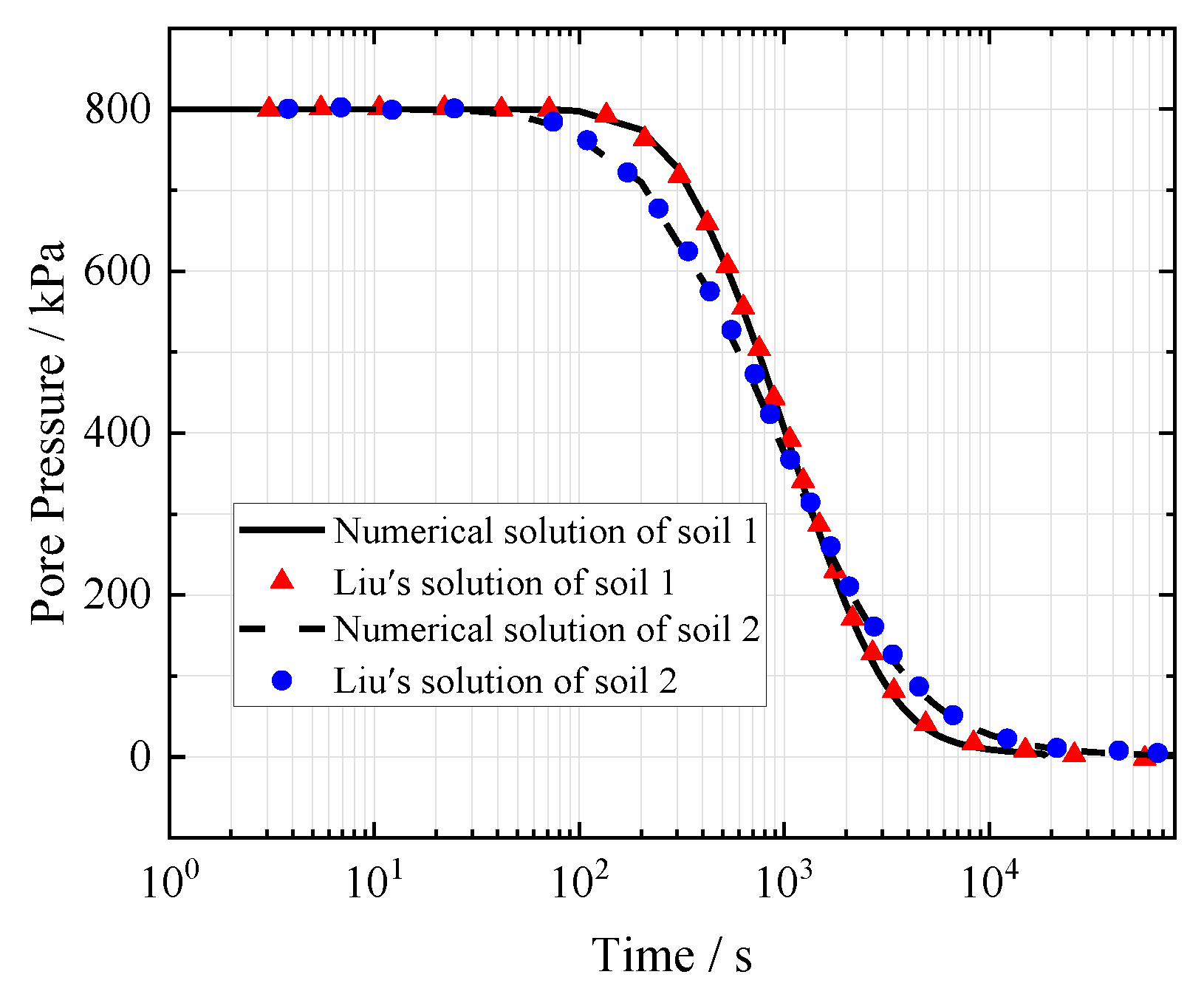
4.3. Verification of the Model and FTCS Algorithm

The validity of the procedure is checked by comparing the calculated numerical solutions to the published data. The first example is from Zhang et al. [29], which involves a partial differential equation, written as follows:

$${\displaystyle \frac{\partial u(x,t)}{\partial t}}=D_{0,t}^{1-r}\left[{\displaystyle \frac{{\partial }^{2}u(x,t)}{\partial x^2}}\right]+G(x,t) 0<x<1, 0<t\le 1$$

(40)

and the associated initial and boundary conditions:

$$\begin{array}{cc}u(0,t)=t^{3+r}+1 \hfill & \\ u(1,t)=\mathrm{e}(t^{3+r}+1)\hfill & 0<t\le 0.5\hfill \\ u(x,0)={\mathrm{e}}^x\hspace{1em}\hfill & 0\le x\le 1\hfill \end{array}$$

(41)

where $G(x,t)={\mathrm{e}}^x\left[(3+r)t^{2+r}-{\displaystyle \frac{t^{r-1}}{\Gamma (r)}}-{\displaystyle \frac{\Gamma (4+r)}{\Gamma (3+2r)}}{t}^{2+2r}\right]$. According to the published work, the analytical solution of Equation (40) is $u(x,t)={\mathrm{e}}^x(t^{3+r}+1)$.

For comparison, Equation (18) needs to be degraded by letting $\alpha =0$, $E_1\to \infty$, $c=0$, and $f\left(x,t\right)=G\left(x,t\right)$. The evolution of $u$ with respect to $c$ are plotted against time in Figure 7. As seen, the solutions given by the proposed numerical procedure agree well with the analytical one when $c=0$.

In addition, when we let $\beta =0$, $E_0\to \infty$, and $f\left(x,t\right)=0$, Equation (18) degrades to a 1D fractional consolidation model, whose mechanical behavior of the soil skeleton is governed by the fractional Kelvin model, and water flow is controlled by classical Darcy’s law. Liu and Yang [30] have obtained a semi-analytical solution of this problem by using the Laplace transform and the numerical inverse Laplace transform method. The parameters of two soil samples are given in

Table 1. Soil parameters of the second example.

Soil Number	h/m	k/(m/s)	α	E/(MPa)	F/(MPa·s)
1	0.02	1 × 10−10	0.13	7.6	4560
2	0.02	4 × 10−11	0.35	17.0	51,000

, and the results are shown in Figure 8. It is found that the results given in the literature and this paper are also consistent.

5. Parametric Study and Discussion

In this section, the rheological consolidation behavior of a single homogeneous soil layer is investigated. All geometrical and material-related parameters are listed in

Table 2. Soil parameters.

h/m	E0/(MPa)	E1/(MPa)	k/(m/s)	kβ/(m/s1−β)	η/(s)
0.5	30	30	6 × 10−9	4.5 × 10−7	2000

, some of which are consistent with Liu et al. [30]. Unless otherwise stated, the default values of $\alpha$ and $\beta$ are 0.5.

For simplicity, a one-stage ramp loading is considered as follows:

$$p\left(t\right)=\left\{\begin{array}{cc}{\displaystyle \frac{p_1}{t_1}}t\hfill & \hfill 0\le t\le t_1\\ p_1\hfill & \hfill t_1<t\end{array}\right.$$

(42)

where $p_1=1 \mathrm{MPa}$ and $t_1=2000 \mathrm{s}$. It is worth pointing out that $u_0=0$ due to ramp loading.

5.1. Influence of the Loading Rate

A wide range of values of $t_1$, from 1000 s to 3000 s, covering rapid to slow loading, has been considered. As the average degree of consolidation defined by settlement ($U_s$) and by excessive pore pressure ($U_p$) is identical in classical Terzaghi’s model, only $U_p$ is presented in this section. According to Hanna et al. [31], the average degree of consolidation $U_p$ at the end of ramp loading is given by the following:

$$\left\{\begin{array}{l}{U}_p=1-{\displaystyle \frac{1}{T_1}}\left[{\displaystyle \sum _{m=0}^{\infty }\left(\frac{2}{M^4}\right)\left(1-e^{-M^2{T}_1}\right)}\right]\\ M={\displaystyle \frac{\left(2m+1\right)\pi }{2}}\\ T_1={\displaystyle \frac{E_{0}c{t}_1}{L^2}}\end{array}\right.$$

(43)

The validity of the proposed procedure is further checked by comparing the calculated $U_p$ at the end of loading stage to the analytical one according to Equation (43). To achieve this, the fractional model needs to be degraded to the Terzaghi’s model by setting $E_1\to \infty$, $k_{\beta }=0$, and $f\left(x,t\right)=0$. The results given by the procedure and Equation (43) are listed in

Table 3. Comparison between numerical and analytical $U_p$.

Time Factor t1/(s)	Numerical Up	Analytical Up
1000	0.203949	0.203900
2000	0.288388	0.288352
3000	0.353064	0.353035

. As seen, the proposed numerical solutions agree well with the analytical ones.

The loading rate has a great influence on the consolidation process, as shown in Figure 9. The higher loading rate results in greater values of $U_p$ and $U_s$ in the loading stage. This occurs because an increase in the loading rate accelerates compression deformation of the soil and accordingly, produces a higher average degree of consolidation. In the holding stage, where the loading conditions are maintained at the same level, a higher $t_1$ accelerates rate of consolidation as all degrees of consolidation tend to asymptotic values.

Moreover, it is noteworthy that in the rheological consolidation model, the average degree of consolidation defined by settlement ($U_s$) and by excessive pore pressure ($U_p$) differs, which contrasts with Terzaghi’s model. Especially as the loading stage and holding stage of each loading rate are distinguished by different colors, it is obvious that $U_p$ remains consistently larger than $U_s$, which indicates that the settlement progresses more slowly than the overall dissipation of excess pore pressure. This is consistent with the work of Cui et al. [32] and is further confirmed in the subsequent case studies.

5.2. Influence of the FDMM Parameters

For simplicity, the subsequent case studies are based on the same loading rate, namely, $t_1=2000 \mathrm{s}$.

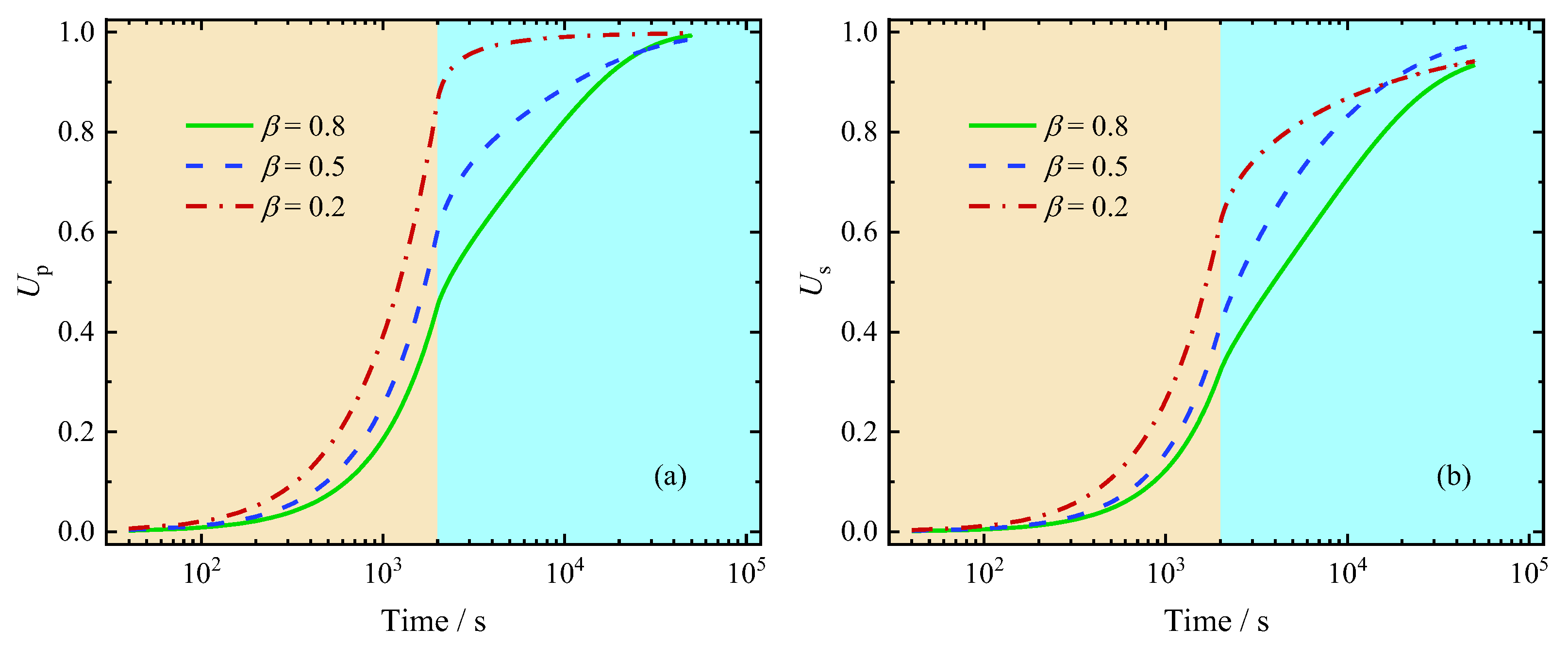
5.2.1. Influence of the Fractional Order $\alpha$

Figure 10 illustrates the effect of the fractional order $\alpha$ on the average degree of consolidation defined by excess pore pressure ($U_p$) and settlement ($U_s$). Generally, the impact of $\alpha$ on $U_p$ and $U_s$ is most pronounced in the holding stage, where $U_s$ consistently changes at a lower rate than $U_p$.

In the loading stage, an increase in $\alpha$ results in a higher value of $U_p$, though this effect is minimal. In the holding stage, the effect of $\alpha$ on $U_p$ remains consistent with that observed in the loading stage, as illustrated in Figure 10a. The effect of $\alpha$ on $U_s$ mimics that of $\alpha$ on $U_p$. This is also consistent with the findings of Cui et al. [32].

Conversely, Figure 10b shows that a decrease in $\alpha$ leads to an increase in $U_s$ in the early loading stage (before 100 s), after which the trend reverses and becomes more pronounced over time. This characteristic has been discussed in the literature [32,33]. They attributed the intersecting phenomenon to the complexity of the fractional derivative-based component model. Overall, this phenomenon appears to be independent of the loading form and is closely related to the consolidation stage.

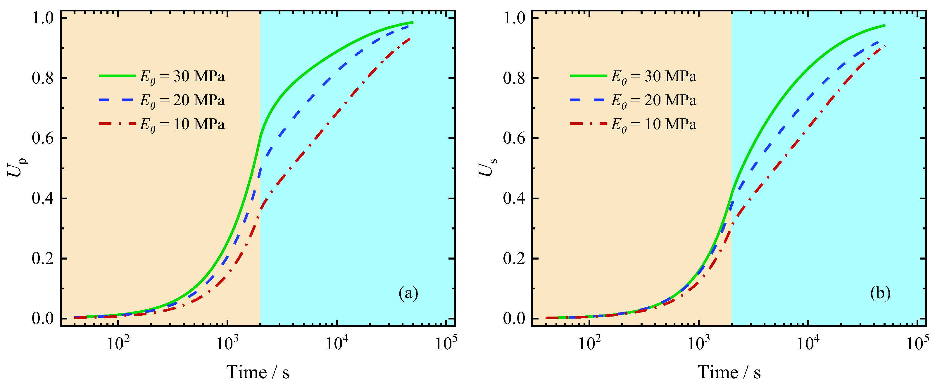
5.2.2. Influence of the Elastic Modulus $E_0$

The larger the elastic modulus $E_0$, the faster the excess pore water pressure dissipates, as shown in Figure 11a. As the elastic modulus $E_0$ increases, the soil skeleton’s resistance to elastic deformation improves, requiring greater effective stress to achieve the same level of elastic deformation. This enhancement accelerates the conversion of excess pore water pressure into effective stress, thereby accelerating the dissipation of excess pore water pressure.

With respect to $U_s$, the general pattern mimics that of $U_p$. An increase in $E_0$ results in a smaller final settlement due to the inverse relationship between the magnitude of elastic deformation and $E_0$, as illustrated in Equation (14). According to the definition of $U_s$, a smaller final settlement leads to a larger $U_s$ at any given time.

5.2.3. Influence of the Elastic Modulus $E_1$

Figure 12a,b depict the variation in the average degree of consolidation $U_p$ and $U_s$ for different elastic moduli $E_1$. Compared to Figure 11a, the influence of $E_1$ on $U_p$ is minimal, as shown in Figure 12a. This is because consolidation is a process that gradually converts excess pore water pressure into effective stress, which primarily counteracts the instantaneous elastic deformation of the soil skeleton. Due to the characteristics of viscous deformation, the effect of $E_1$ on the dissipation of excess pore water pressure (i.e., the generation of effective stress) is limited. Therefore, an increase in $E_1$ primarily affects the viscous deformation while having minimal influence on the dissipation of excess pore water pressure.

Figure 12b shows that a larger $E_1$ results in a lower settlement. This is because an increase in $E_1$ reduces viscous deformation and accordingly, limits the final deformation. As a result, the reduction in final settlement accelerates the average degree of consolidation $U_s$.

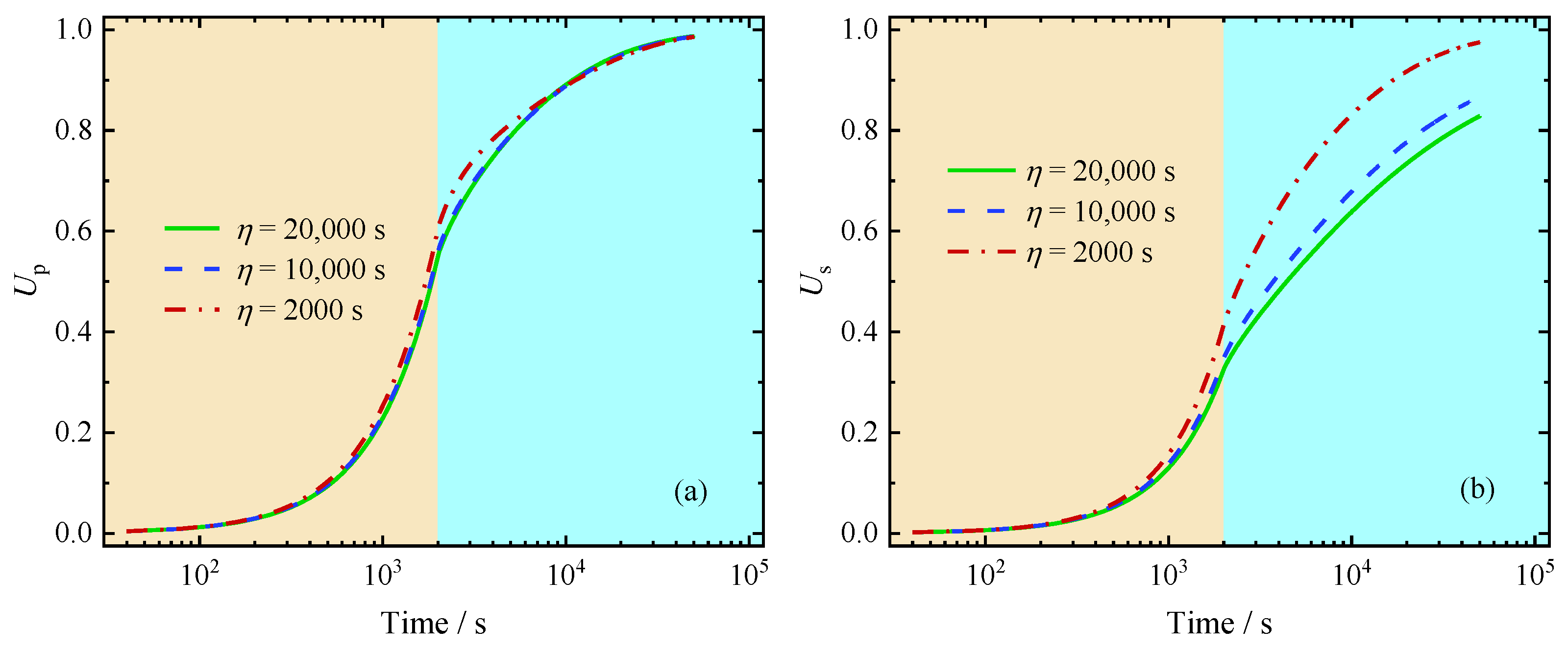
5.2.4. Influence of the Viscosity Time $\eta$

Three values of viscosity time $\eta =2000 \mathrm{s}$, $\mathrm{10,000} \mathrm{s}$, and $\mathrm{20,000} \mathrm{s}$ were chosen for analysis. The viscosity time is associated with the thickness of the bound water around the soil particles [34]. Physically, a thinner bound water film increases soil viscosity, making it more difficult for the soil particle arrangement. Consequently, the viscosity time $\eta$ primarily affects the viscous deformation rate of the soil skeleton, with minimal impact on the dissipation of excess pore water pressure. As illustrated in Figure 13, the settlement decreases as viscosity time $\eta$ increases, leading to a smaller $U_s$.

5.3. Influence of the FDDM Parameters

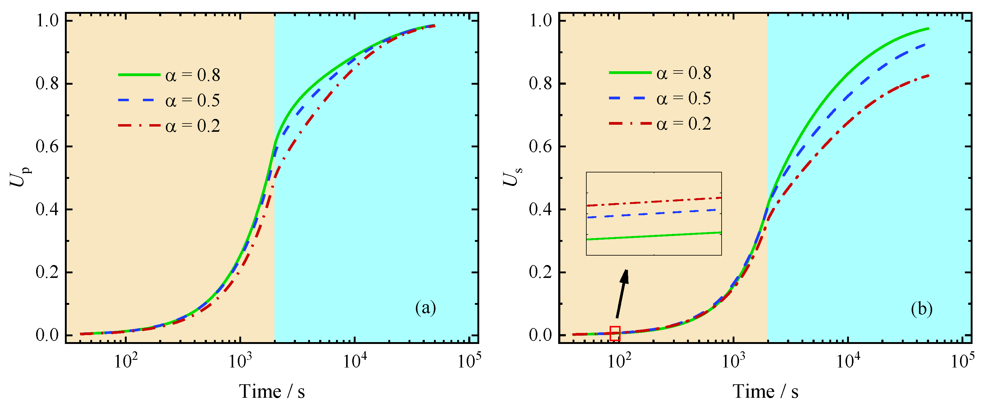
5.3.1. Influence of the Fractional Order $\beta$

The parameter $\beta$ reflects the degree of change in pore structure. A higher fractional order $\beta$ results in a more significant reduction in the permeability of the soil, which slows the rate of $U_p$, as shown in Figure 14a. However, in the final consolidation stage, this trend reverses. This occurs because the residual excess pore pressure is minimal at the end of the consolidation process, and the hydraulic gradient is significantly reduced. As a result, the dissipation of excess pore pressure slows down, leading to a decrease in the rate of $U_p$.

Figure 14b exhibits a pattern consistent with Figure 14a. The reversal pattern becomes more pronounced in the final consolidation stage. This can be attributed to the fact that the compression of soft soil typically occurs after the drainage of water. Even if the excess pore pressure has dissipated, the viscous deformation of the soil skeleton persists.

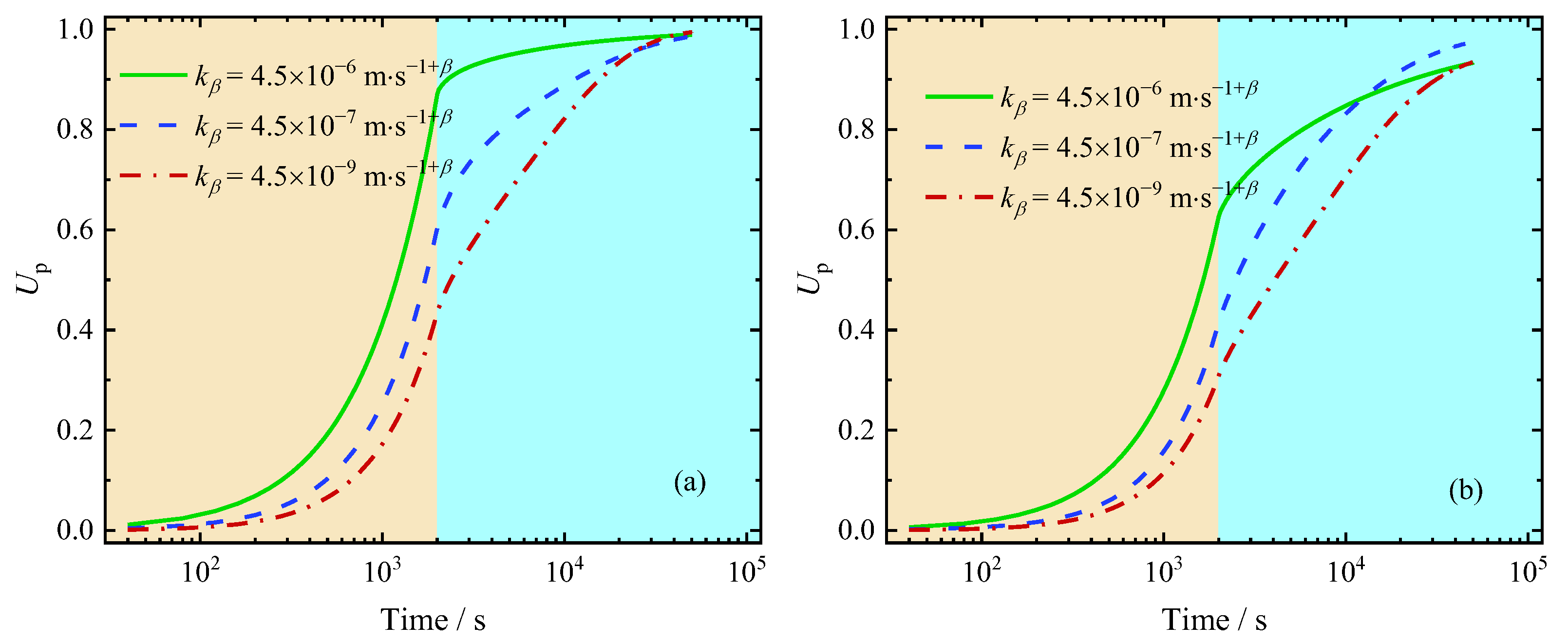
5.3.2. Influence of the Abnormal Permeability Coefficient $k_{\beta }$

A higher permeability coefficient indicates a faster dissipation of excess pore pressure, as shown in Figure 15. Overall, the effect of the abnormal permeability coefficient $k_{\beta }$ is similar to that of the fractional order $\beta$. Although $k_{\beta }$ affects the dissipation rate of excess pore pressure, the total consolidation time remains within the same order of magnitude. This suggests that between the two permeability coefficients, $k$ and $k_{\beta }$, it is $k$ that predominantly governs the consolidation process.

6. Discussion

The consolidation model proposed in this paper integrates fractional constitutive behavior of both the soil skeleton and water flow, enhancing the model to capture memory effects and anomalous diffusion during consolidation. We presented a detailed numerical implementation and conducted the parametric studies for the model.

Nevertheless, this study has certain limitations. The numerical solution is computationally demanding due to the integration of the fractional Merchant model and the fractional Darcy model. This complexity is further amplified over longer time spans, as the memory effect inherent in fractional derivatives requires referencing all past time points during computations. Additionally, the model is confined to one-dimensional analysis, and the finite difference method employed may face difficulties when applied to problems with complex geometries or multidimensional domains.

Future work could focus on developing more efficient numerical algorithms for the fractional consolidation model, enhancing its applicability to more complex engineering scenarios.

7. Conclusions

In this study, Terzaghi’s one-dimensional consolidation model was revisited by taking the time-dependent deformation of the soil skeleton and the abnormal diffusion process of water flow into account. The rheological consolidation model was established, and the corresponding numerical procedure was also proposed. After comprehensive parametric studies, main conclusions were drawn as follows:

(1)

Throughout the consolidation process, $U_p$ consistently exceeds $U_s$, indicating that the excess pore pressure dissipation process occurs ahead of soil settlement. This phenomenon becomes more pronounced as $\alpha$, $E_0$ and $E_1$ decrease, while $k_{\beta }$ and $\eta$ increase. Furthermore, a higher loading rate results in greater degrees of consolidation during the loading stage but a slower consolidation rate in the holding stage.

(2)

The impact of elastic modulus $E_1$ and the viscosity time $\eta$ on the consolidation process is primarily observed in the soil settlement during the holding stage. As $E_1$ increases or $\eta$ decreases, the soil settlement rate increases, reflecting the critical role of viscoelastic properties in long-term consolidation behavior.

(3)

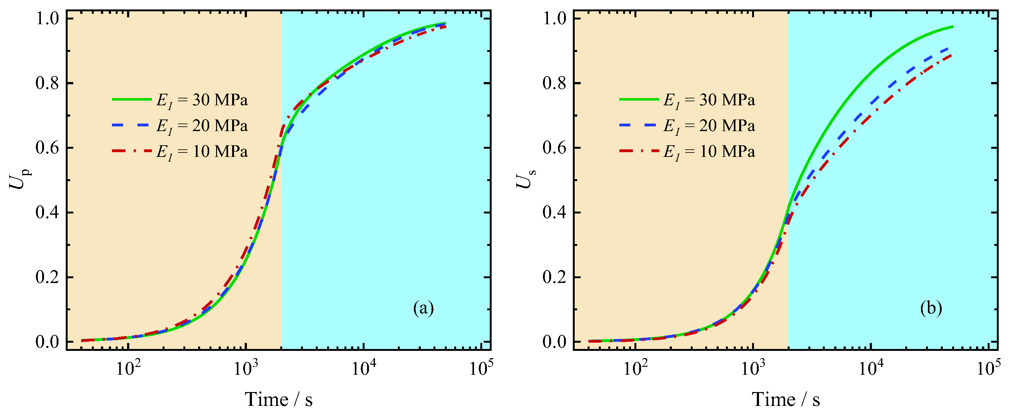
Both in the loading and holding stages, $E_0$ significantly impacts excess pore pressure dissipation and settlement rates, with an increase in $E_0$ accelerating both. In contrast, $E_1$ affects only the settlement rate during the holding stage, where a higher $E_1$ speeds up soil settlement. This difference can be attributed to the fact that changes in $E_0$ influence the elastic deformation of the soil, while changes in $E_1$ primarily affect its viscous deformation.

(4)

With the decrease in $\beta$ and the increase in $k_{\beta }$, the consolidation rate of the soil accelerates in the early and middle stages of the consolidation process but slows down in the final stage. Between the two permeability coefficients, $k$ and $k_{\beta }$, $k$ predominantly governs the consolidation rate, suggesting that traditional permeability $k$ remains a key factor even in the presence of memory effects.

References

1. Terzaghi, K. Theory of consolidation. In Theoretical Soil Mechanics; John Wiley& Sons: New York, NY, USA, 1943; pp. 265–296. [Google Scholar]
2. Yuan, J.; Ye, L.; Hu, G.; Ying-Guang, F. Experimental study on the influence of granulometric and material compositions on soil rheological properties. Soil Mech. Found. Eng. 2020, 57, 35–42. [Google Scholar] [CrossRef]
3. Ter-Martirosyan, Z.; Ter-Martirosyan, A. Rheological properties of soil subject to shear. Soil Mech. Found. Eng. 2013, 49, 219. [Google Scholar] [CrossRef]
4. Lanes, R.M.; Greco, M.; Almeida, V.D. Viscoelastic soil–structure interaction procedure for building on footing foundations considering consolidation settlements. Buildings 2023, 13, 813. [Google Scholar] [CrossRef]
5. Ter-Martirosyan, Z.G.; Ter-Martirosyan, A.Z.; Kurilin, N.O. Predicting the settlement and long-term bearing capacity of a base of foundation of finite width. Soil Mech. Found. Eng. 2021, 58, 190–195. [Google Scholar] [CrossRef]
6. Huang, W.; Wen, K.; Deng, X.; Li, J.; Jiang, Z.; Li, Y.; Li, L.; Amini, F. Constitutive model of lateral unloading creep of soft soil under excess pore water pressure. Math. Probl. Eng. 2020, 2020, 5017546. [Google Scholar] [CrossRef]
7. Yu, Y.-Y.; Luo, C.-L.; Cui, W.-H.; Tao, J.-Y.; Zhang, T.-H. Study on creep characteristics and component model of saline soil in hexi corridor. Sci. Rep. 2023, 13, 18067. [Google Scholar] [CrossRef]
8. Ding, P.; Xu, R.; Ju, L.; Qiu, Z.; Cheng, G.; Zhan, X. Semi-analytical analysis of fractional derivative rheological consolidation considering the effect of self-weight stress. Int. J. Numer. Anal. Methods Geomech. 2021, 45, 1049–1066. [Google Scholar] [CrossRef]
9. Wang, P.; Tang, Y.; Ren, P.; Zhang, H. An isochronous stress ratio logarithmic strain curve based clay creep model considering the effects of hardening and damage. Sci. Rep. 2024, 14, 7057. [Google Scholar] [CrossRef]
10. Huang, M.; Lv, C.; Zhou, S.; Zhou, S.; Kang, J. One-dimensional consolidation of viscoelastic soils incorporating Caputo-Fabrizio fractional derivative. Appl. Sci. 2021, 11, 927. [Google Scholar] [CrossRef]
11. Wang, L.; Chen, H.; Liu, S.; Yu, Y. Rheological consolidation analysis of saturated clay ground under cyclic loading based on the fractional order Kelvin model. Int. J. Numer. Anal. Methods Geomech. 2024, 48, 1814–1832. [Google Scholar] [CrossRef]
12. Ding, P.; Xu, R.; Zhu, Y.; Wen, M. Fractional derivative modelling for rheological consolidation of multilayered soil under time-dependent loadings and continuous permeable boundary conditions. Acta Geotech. 2022, 17, 2287–2304. [Google Scholar] [CrossRef]
13. Hu, S.; Li, X.; Bai, B.; Shi, L.; Liu, M.; Wu, H. A modified true triaxial apparatus for measuring mechanical properties of sandstone coupled with Co2-H2o biphase fluid. Greenh. Gases Sci. Technol. 2017, 7, 78–91. [Google Scholar] [CrossRef]
14. Han, Z.; Li, J.; Li, Y.; Gu, X.; Chen, X.; Wei, C. Assessment of the size selectivity of eroded sediment in a partially saturated sandy loam soil using scouring experiments. Catena 2021, 201, 105234. [Google Scholar] [CrossRef]
15. Ranaivomanana, H.; Razakamanantsoa, A.; Amiri, O. Permeability prediction of soils including degree of compaction and microstructure. Int. J. Geomech. 2017, 17, 04016107. [Google Scholar] [CrossRef]
16. van Verseveld, C.J.W.; Gebert, J. Effect of compaction and soil moisture on the effective permeability of sands for use in methane oxidation systems. Waste Manag. 2020, 107, 44–53. [Google Scholar] [CrossRef]
17. Xie, J.; Li, Q.; Li, T.; Zhao, Z. Lattice boltzmann simulation of non-darcy flow in stochastically generated three-dimensional granular porous media. J. Porous Media 2021, 24, 93–104. [Google Scholar] [CrossRef]
18. Gao, M.; Zhang, C.; Oh, J. Assessments of the effects of various fracture surface morphology on single fracture flow: A review. Int. J. Min. Sci. Technol. 2023, 33, 1–29. [Google Scholar] [CrossRef]
19. Muzemder, A.T.M.S.H.; Singh, K. Intra-pore tortuosity and diverging-converging pore geometry controls on flow enhancement due to liquid boundary slip. J. Hydrol. 2021, 598, 126475. [Google Scholar] [CrossRef]
20. Zhou, H.W.; Yang, S.; Zhang, S.Q. Modeling non-Darcian flow and solute transport in porous media with the Caputo–Fabrizio derivative. Appl. Math. Model. 2019, 68, 603–615. [Google Scholar] [CrossRef]
21. Di Giuseppe, E.; Moroni, M.; Caputo, M. Flux in porous media with memory: Models and experiments. Transp. Porous Media 2010, 83, 479–500. [Google Scholar] [CrossRef]
22. Wang, R.; Zhou, H.-w.; Zhuo, Z.; Xue, D.-j.; Yang, S. Finite difference method for space-fractional seepage process in unsaturated soil. Chin. J. Geotech. Eng. 2020, 42, 1759–1764. [Google Scholar]
23. Kim, P.; Kim, H.-S.; Pak, C.-U.; Paek, C.-H.; Ri, G.-H.; Myong, H.-B. Analytical solution for one-dimensional nonlinear consolidation of saturated multi-layered soil under time-dependent loading. J. Ocean Eng. Sci. 2021, 6, 21–29. [Google Scholar] [CrossRef]
24. Cui, P.; Cao, W.; Lin, C.; Liu, Y.; Chen, M.; Zhang, J. 1d elastic viscoplastic consolidation analysis of bi-layered soft ground under time-dependent drainage boundary and ramp load. Int. J. Numer. Anal. Methods Geomech. 2024, 48, 55–77. [Google Scholar] [CrossRef]
25. Li, C.; Qian, D.; Chen, Y. On Riemann-Liouville and Caputo derivatives. Discret. Dyn. Nat. Soc. 2011, 2011, 562494. [Google Scholar] [CrossRef]
26. Koeller, R.C. Applications of fractional calculus to the theory of viscoelasticity. J. Appl. Mech. 1984, 51, 299–307. [Google Scholar] [CrossRef]
27. Alaimo, G.; Piccolo, V.; Cutolo, A.; Deseri, L.; Fraldi, M.; Zingales, M. A fractional order theory of poroelasticity. Mech. Res. Commun. 2019, 100, 103395. [Google Scholar] [CrossRef]
28. Iaffaldano, G.; Caputo, M.; Martino, S. Experimental and theoretical memory diffusion of water in sand. Hydrol. Earth Syst. Sci. 2006, 10, 93–100. [Google Scholar] [CrossRef]
29. Zhang, Y.-N.; Sun, Z.-Z.; Wu, H.-W. Error estimates of Crank–Nicolson-type difference schemes for the subdiffusion equation. SIAM J. Numer. Anal. 2011, 49, 2302–2322. [Google Scholar] [CrossRef]
30. Liu, Z.; Yang, Q. One-dimensional rheological consolidation analysis of saturated clay using fractional order Kelvin’s model. Rock Soil Mech. 2017, 38, 3680–3687, 3697. [Google Scholar]
31. Hanna, D.; Sivakugan, N.; Lovisa, J. Simple approach to consolidation due to constant rate loading in clays. Int. J. Geomech. 2013, 13, 193–196. [Google Scholar] [CrossRef]
32. Cui, P.; Liu, Z.-Y.; Zhang, J.-C.; Fan, Z.-C. Analysis of one-dimensional rheological consolidation of double-layered soil with fractional derivative Merchant model and non-Darcian flow described by non-Newtonian index Merchant. J. Cent. South Univ. 2021, 28, 284–296. [Google Scholar] [CrossRef]
33. Liu, Z.; Cui, P.; Zhang, J.; Xia, Y. Consolidation analysis of ideal sand-drained ground with fractional-derivative Merchant model and non-Darcian flow described by non-Newtonian index. Math. Probl. Eng. 2019, 2019, 5359076. [Google Scholar] [CrossRef]
34. Zhang, S.; Pei, H. Determining the bound water content of montmorillonite from molecular simulations. Eng. Geol. 2021, 294, 106353. [Google Scholar] [CrossRef]
Figure 1. (a) Schematic diagram of Kelvin model (b) Schematic diagram of fractional derivative Merchant model.
Fractalfract 09 00233 g001
Figure 2. Influence of the fractional order ɑ on creep strain.
Fractalfract 09 00233 g002
Figure 3. (a) Fitting of Published Dataset 1 from Iaffaldano’s Paper (b) Fitting of Published Dataset 2 from Iaffaldano’s Paper (c) Fitting of Published Dataset 1 from Giuseppe’s Paper (d) Fitting of Published Dataset 2 from Giuseppe’s Paper.
Fractalfract 09 00233 g003
Figure 4. Schematic diagram of 1D consolidation model.
Fractalfract 09 00233 g004
Figure 5. Multi-stage loading scheme.
Fractalfract 09 00233 g005
Figure 6. Schematic diagram of finite difference grids for a one-dimensional problem.
Fractalfract 09 00233 g006
Figure 7. Comparison between the numerical results given by the proposed procedure to the analytical ones.
Fractalfract 09 00233 g007
Figure 8. Comparison between the numerical results given by the proposed procedure to the published work.
Fractalfract 09 00233 g008
Figure 9. Influence of loading rate on average degree of consolidation: (a) Up (b) Us.
Fractalfract 09 00233 g009
Figure 10. Influence of fractional order α on average degree of consolidation: (a) Up (b) Us.
Fractalfract 09 00233 g010
Figure 11. Influence of elastic modulus E 0 on average degree of consolidation: (a) Up (b) Us.
Fractalfract 09 00233 g011
Figure 12. Influence of elastic modulus E 1 on average degree of consolidation: (a) Up (b) Us.
Fractalfract 09 00233 g012
Figure 13. Influence of viscosity time η on average degree of consolidation: (a) Up (b) Us.
Fractalfract 09 00233 g013
Figure 14. Influence of fractional order β on average degree of consolidation: (a) Up (b) Us.
Fractalfract 09 00233 g014
Figure 15. Influence of abnormal permeability coefficient k β on average degree of consolidation: (a) Up (b) Us.
Fractalfract 09 00233 g015