


A Fireline Displacement Model to Predict Fire Spread


 ,
,  , and
, and 
Abstract
1. Introduction
2. Fireline Displacement Model
2.1. Modeling Approach
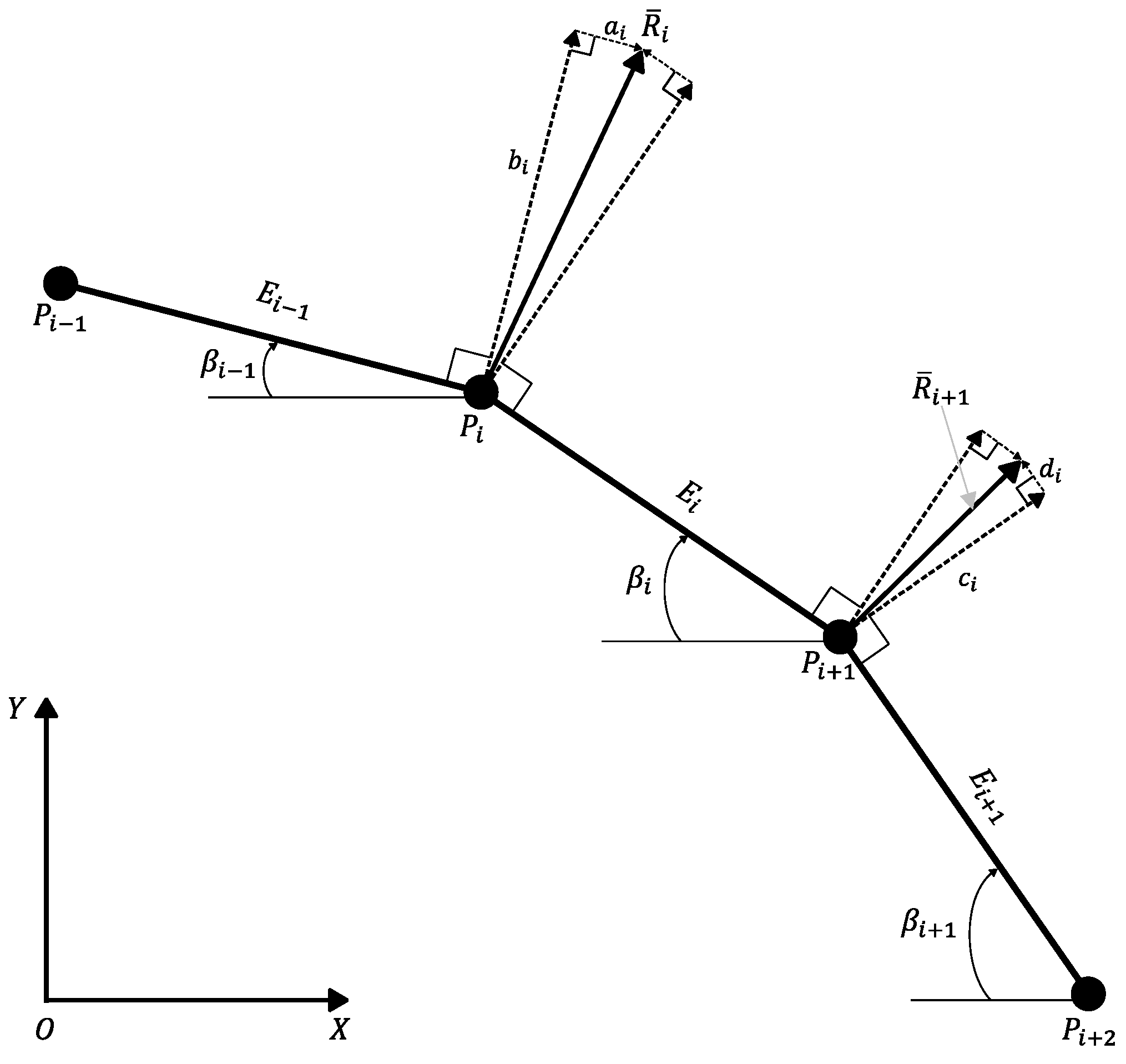
2.2. Displacement of a Fireline Element
2.3. Analysis of Fireline Extension
2.4. Estimation of Local Value of Fireline Extension
2.4.1. Approximate Value of the Modulus of the ROS
2.4.2. Approximate Value of the Direction of the ROS
2.4.3. Extension of the Reference Element Containing Q1
2.5. Fireline Rotation Law
3. Materials and Methods
3.1. Laboratory Experiments
3.2. Numerical Model
3.2.1. Calculation of Section 1
Subsection S1.1
Subsection S1.2
3.2.2. Calculation of Section 2
4. Results
4.1. Experimental Results
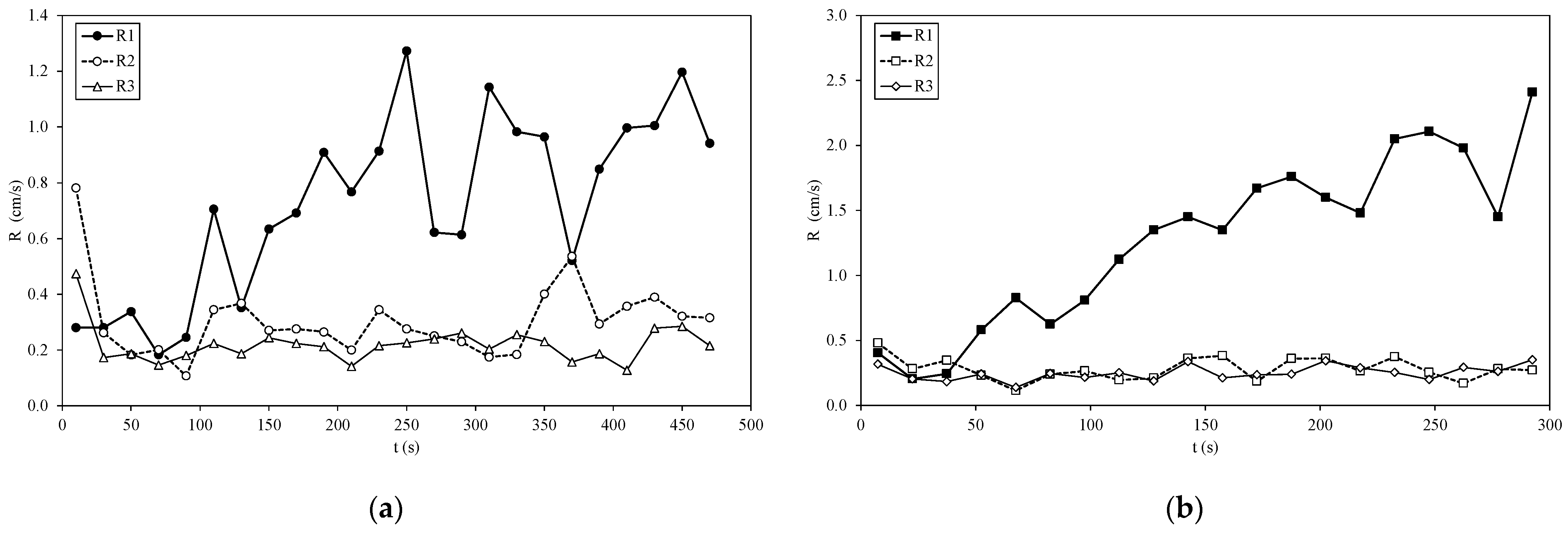
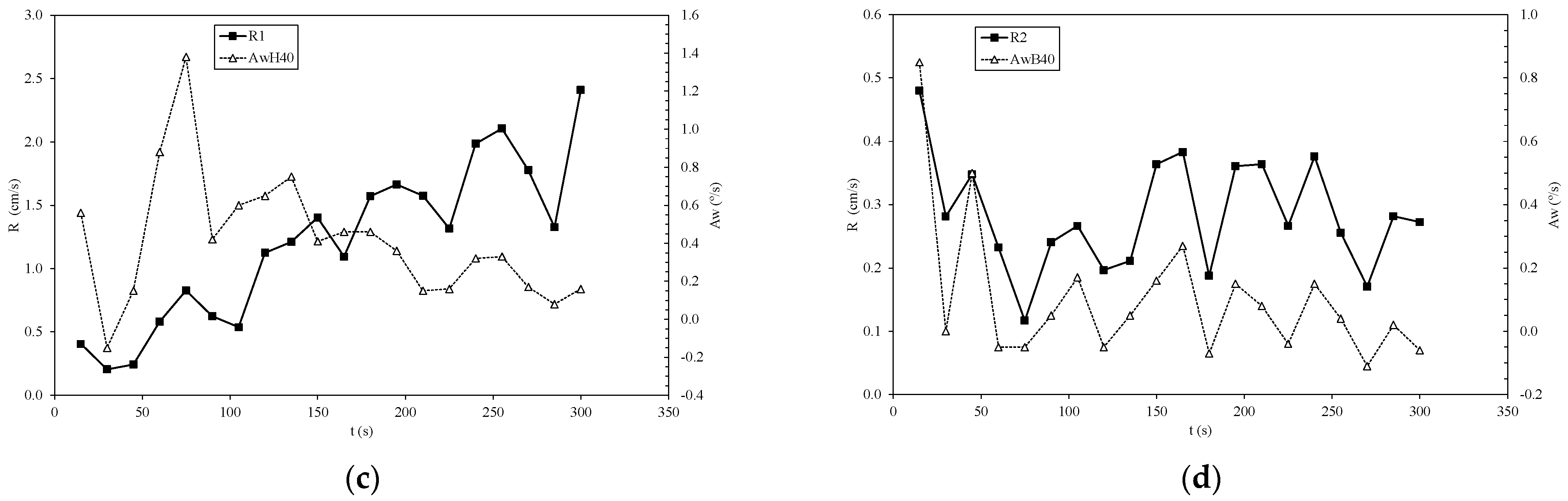
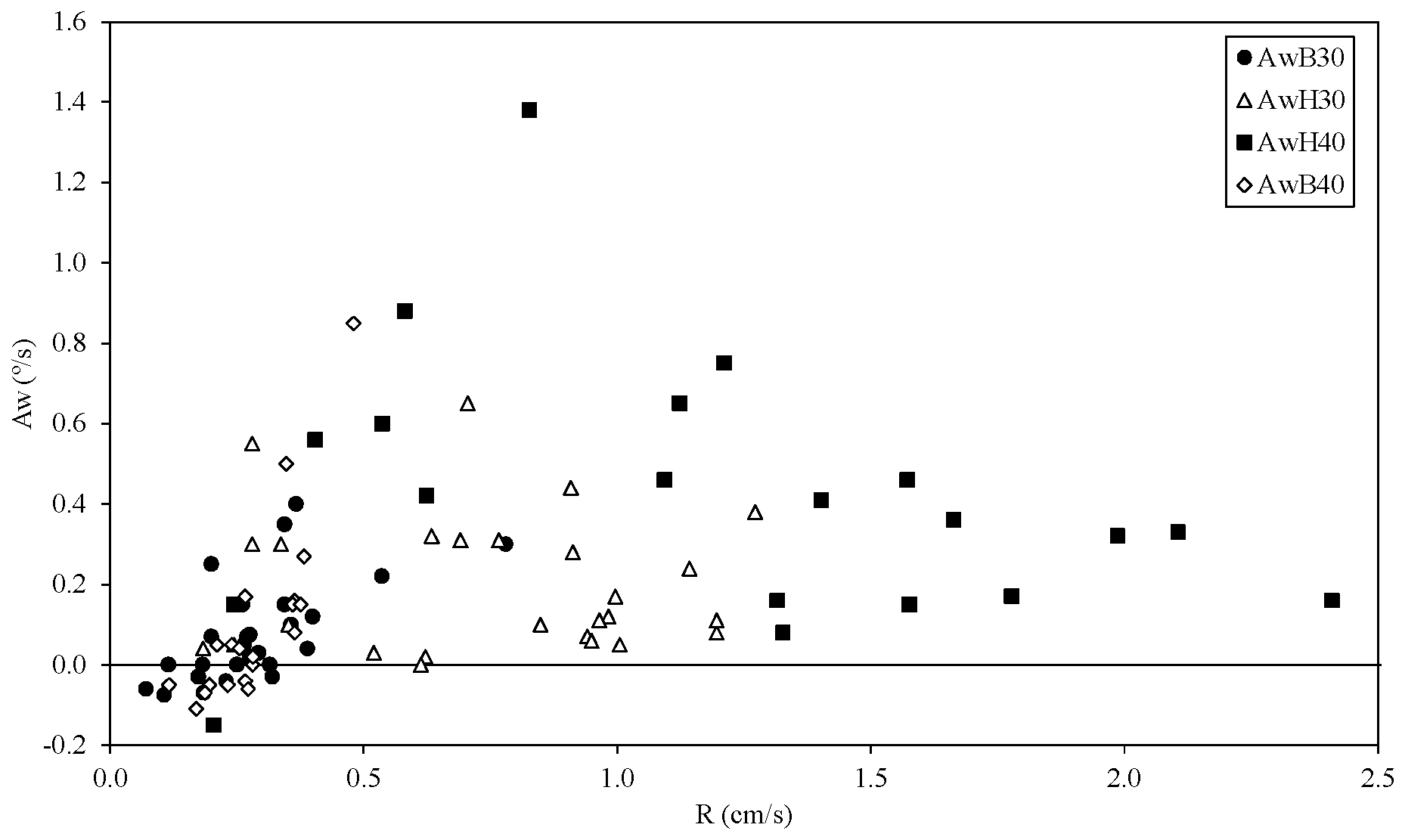
4.1.1. Rate of Spread Results
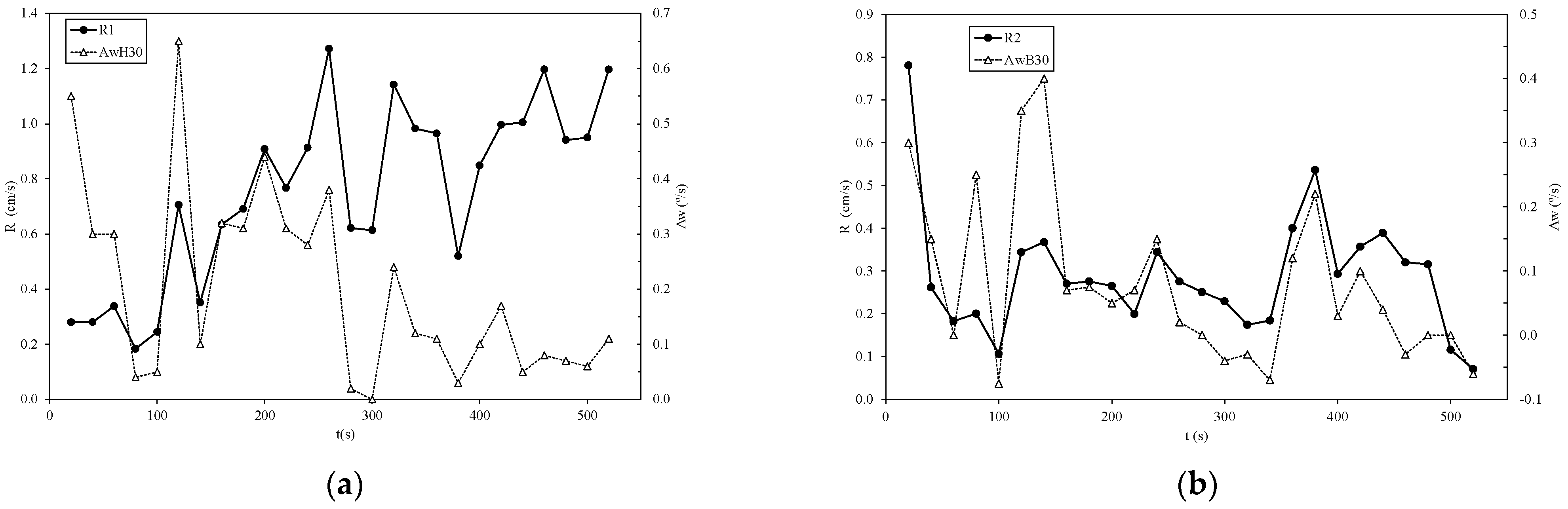
4.1.2. Fireline Rotation Results
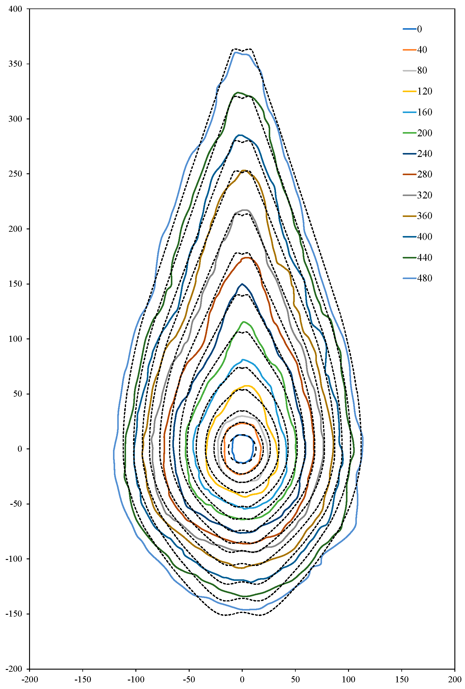
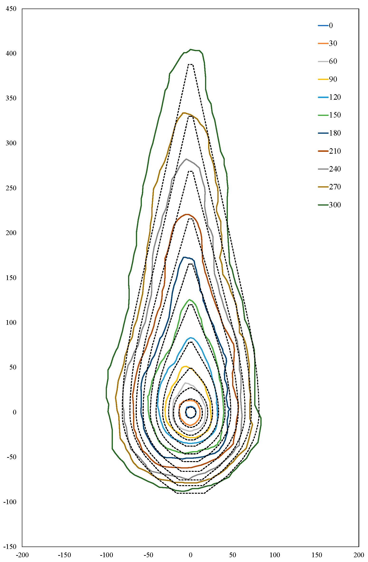
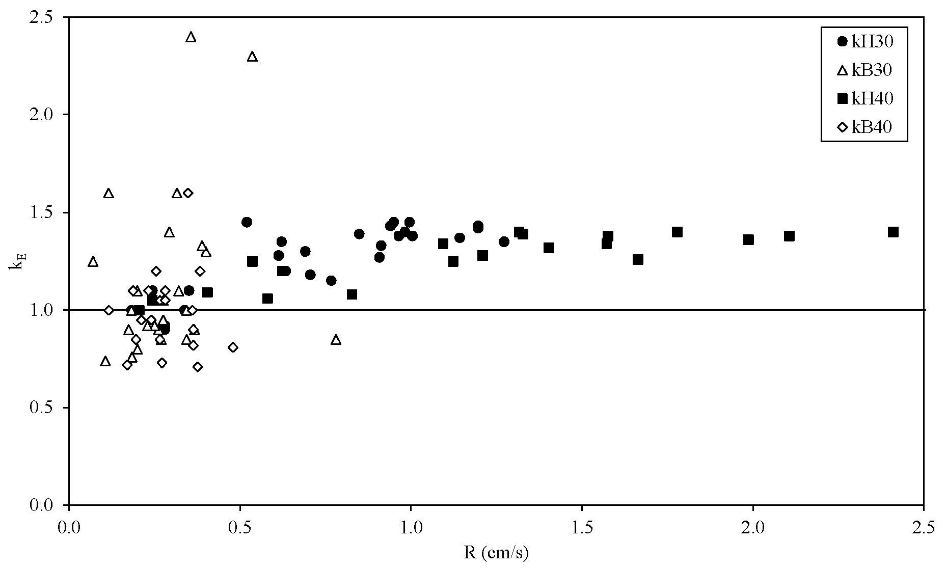
4.2. Numerical Results
5. Discussion
6. Conclusions
Author Contributions
Funding
Institutional Review Board Statement
Informed Consent Statement
Data Availability Statement
Acknowledgments
Conflicts of Interest
Nomenclature
| a1 | Empirical parameter in Equations (28) and (30) |
| a3 | Empirical parameter in Equations (29) and (30) |
| Aw | Empirical coefficient |
| b1 | Exponent in Equations (28) and (30) |
| b2 | Exponent in Equations (29) and (30) |
| ds | Fireline element extension during a time step |
| ds1a | Fireline extension of element E1a |
| dst | Fireline extension due to translation |
| dsω | Fireline extension due to rotation |
| Ei | Fireline element limited by points Pi and Pi+1 |
| FLE | Fireline element |
| K | Number of fireline elements |
| kE | FLE extension correction coefficient |
| ko | Constant associated to extension of element E1a |
| m1 | Empirical parameter of the model |
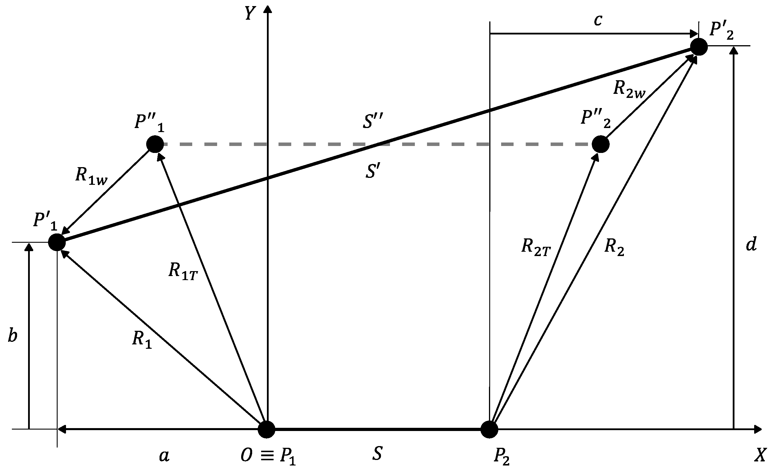
| P1 | Point P1 in the fireline at time step t |
| P1′ | |
| P1″ | |
| P2 | Point P2 in the fireline at time step t |
| P2′ | |
| P2″ | |
| R | Modulus of the ROS |
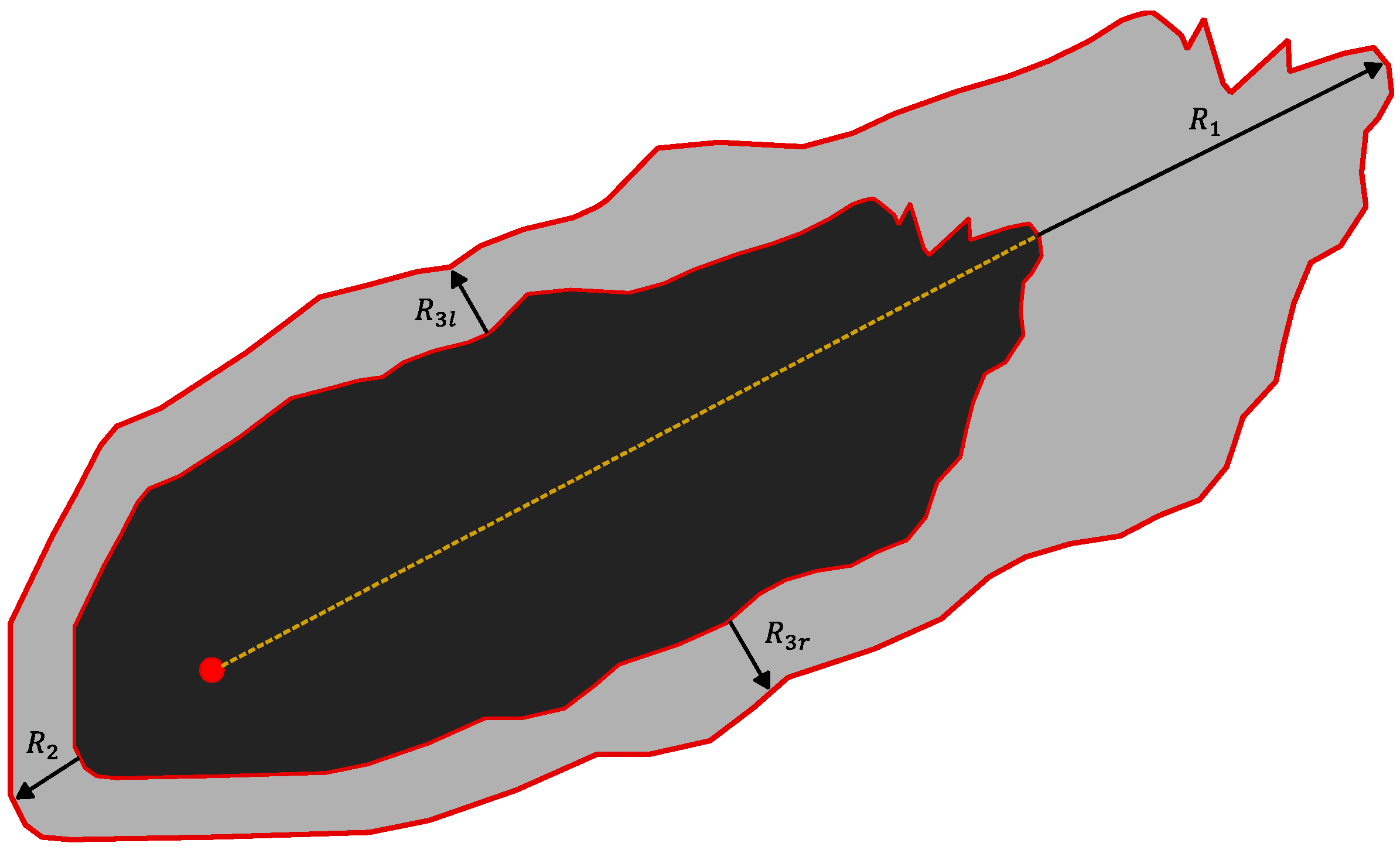
| R1 | Head fire ROS |
| R2 | Backfire ROS |
| R3 | Lateral fire ROS |
| Ro | Initial radius of the fire perimeter |
| Ro | Basic rate of spread in no slope and no wind conditions |
| ROS | Rate of spread |
| s | Extension (length) of a fireline element at time step t |
| s′ | Extension (length) of a fireline element at time step t + |
| s1a″ | after translation |
| t | Time |
| u | Local flow velocity parallel to fuel bed |
| ux | Local flow velocity component parallel to the fireline element |
| uy | Local flow velocity component perpendicular to the fireline element |
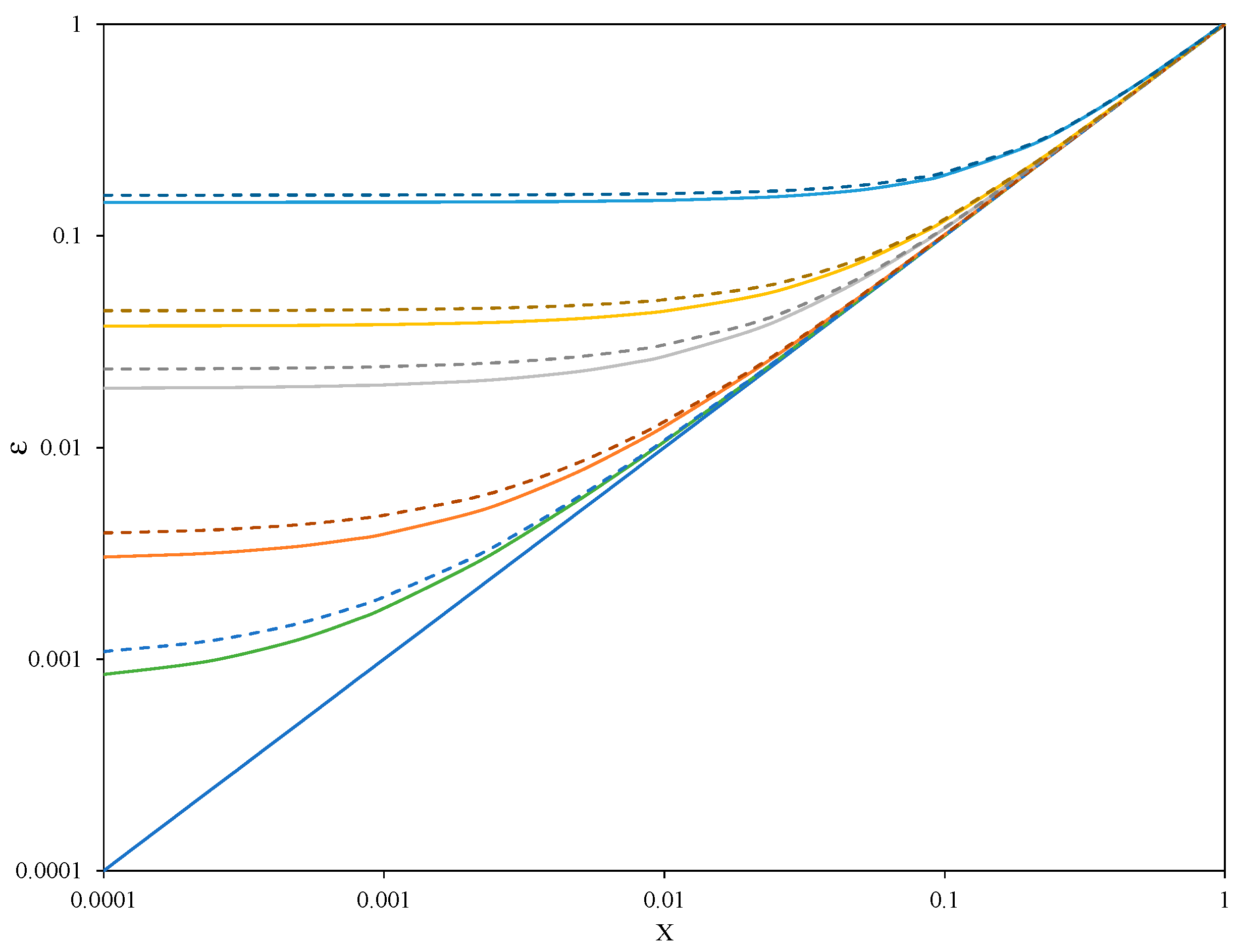
| X | Parameter associated to translation |
| xi | Coordinate at y axis |
| xi′ | Coordinate at y axis at time step t + |
| Y | Parameter associated to rotation |
| yi | Coordinate at y axis |
| yi′ | Coordinate at y axis at time step t + |
| Greek letters | |
| β | Angle between the local rate of spread and OYo axis |
| Δt | Time variation or time step |
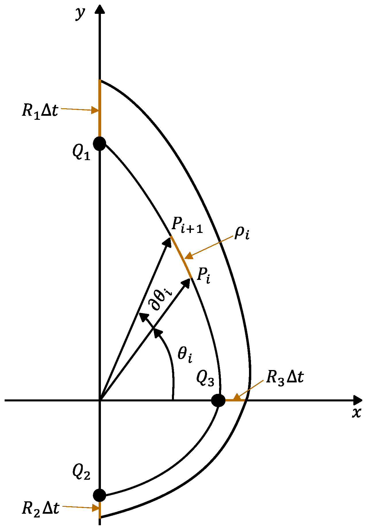
| θ | Angle from the origin of the cartesian plane |
| θi | Radial coordinate associated to each point |
| εc | Corrected fireline extension coefficient |
| εo | Fireline extension coefficient as function of ko |
| ε | Fireline extension coefficient |
| ω | Rotational velocity |
| ξ | Angular coordinate |
References
- Pastor, E.; Zárate, L.; Planas, E.; Arnaldos, J. Mathematical models and calculation systems for the study of wildland fire behaviour. Prog. Energy Combust. Sci. 2003, 29, 139–153. [Google Scholar] [CrossRef]
- Arroyo, L.A.; Pascual, C.; Manzanera, J.A.; Manzanera, A.; Arroyo, L.A.; Pascual, C. Fire models and methods to map fuel types: The role of remote sensing. For. Ecol. Manag. 2008, 256, 1239–1252. [Google Scholar] [CrossRef]
- Sullivan, A.L. Wildland surface fire spread modelling, 1990–2007. 1: Physical and quasi-physical models. Int. J. Wildl. Fire 2009, 18, 349. [Google Scholar] [CrossRef]
- Sullivan, A.L. Wildland surface fire spread modelling, 1990–2007. 2: Empirical and quasi-empirical models. Int. J. Wildl. Fire 2009, 18, 369. [Google Scholar] [CrossRef]
- Sullivan, A.L. Wildland surface fire spread modelling, 1990–2007. 3: Simulation and mathematical analogue models. Int. J. Wildl. Fire 2009, 18, 387. [Google Scholar] [CrossRef]
- Finney, M.A. FARSITE: Fire Area Simulator-Model Development and Evaluation; Res. Pap. RMRS; Department of Agriculture, Forest Service, Rocky Mountain Research Station: Ogden, UT, USA, 1998; pp. 1–36. [Google Scholar]
- Finney, M.A. An Overview of FlamMap Fire Modeling Capabilities. In Proceedings of the Fuels Management—How to Measure Success: Conference Proceedings, Portland, OR, USA, 28–30 March 2006; pp. 213–220. [Google Scholar]
- Noonan-Wright, E.K.; Opperman, T.S.; Finney, M.A.; Zimmerman, G.T.; Seli, R.C.; Elenz, L.M.; Calkin, D.E.; Fiedler, J.R. Developing the US Wildland Fire Decision Support System. J. Combust. 2011, 2011, 168473. [Google Scholar] [CrossRef]
- Ramírez, J.; Monedero, S.; Buckley, D. New approaches in fire simulations analysis with Wildfire Analyst. In Proceedings of the 5th International Wildland Fire Conference, Sun City, South Africa, 9–13 May 2011; pp. 9–13. [Google Scholar]
- Andrews, P.L. Current status and future needs of the BehavePlus Fire Modeling System. Int. J. Wildl. Fire 2014, 23, 21. [Google Scholar] [CrossRef]
- Lopes, A.M.G.; Cruz, M.G.; Viegas, D.X. FireStation—An integrated software system for the numerical simulation of fire spread on complex topography. Environ. Model. Softw. 2002, 17, 269–285. [Google Scholar] [CrossRef]
- Lopes, A.M.G.; Ribeiro, L.M.; Viegas, D.X.; Raposo, J.R. Simulation of forest fire spread using a two-way coupling algorithm and its application to a real wildfire. J. Wind Eng. Ind. Aerodyn. 2019, 193, 103967. [Google Scholar] [CrossRef]
- Rothermel, R.C. A Mathematical Model for Predicting Fire Spread in Wildland Fuels; USDA Forest Service, Research Paper INT-115; Intermountain Forest and Range Experiment Station: Ogden, UT, USA, 1972. [Google Scholar]
- Rothermel, R.C. How to Predict the Spread and Intensity of Forest and Range Fires; Gen. Tech. Rep. INT-143; U.S. Department of Agriculture, Forest Service, Intermountain Forest and Range Experiment Station: Ogden, UT, USA, 1983; 161p.
- Andrews, P.L. BEHAVE: Fire Behavior Prediction and Fuel Modeling System-BURN Subsystem, Part 1; General Technical Report INT-194; U.S. Department of Agriculture, Forest Service, Intermountain Research Station: Ogden, UT, USA, 1986; 130p.
- Viegas, D.X.F.C.; Raposo, J.R.N.; Ribeiro, C.F.M.; Reis, L.C.D.; Abouali, A.; Viegas, C.X.P. On the non-monotonic behaviour of fire spread. Int. J. Wildl. Fire 2021, 30, 702–719. [Google Scholar] [CrossRef]
- Xavier Viegas, D. A Mathematical Model For Forest Fires Blowup. Combust. Sci. Technol. 2004, 177, 27–51. [Google Scholar] [CrossRef]
- Viegas, D.X. Parametric study of an eruptive fire behaviour model. Int. J. Wildl. Fire 2006, 15, 169. [Google Scholar] [CrossRef]
- Green, D.G.; Gill, A.M.; Noble, I.R. Fire shapes and the adequacy of fire-spread models. Ecol. Modell. 1983, 20, 33–45. [Google Scholar] [CrossRef]
- Richards, G. A General Mathematical Framework for Modeling Two-Dimensional Wildland Fire Spread. Int. J. Wildl. Fire 1995, 5, 63. [Google Scholar] [CrossRef]
- Anderson, D.H.; Catchpole, E.A.; De Mestre, N.J.; Parkes, T. Modelling the spread of grass fires. J. Aust. Math. Soc. Ser. B Appl. Math. 1982, 23, 451–466. [Google Scholar] [CrossRef]
- Alexander, M.E. Estimating the length-to-breadth ratio of elliptical forest fire patterns. In Proceedings of the Eight Conference on Fire and Forest Meteorology, Detroit, MI, USA, 29 April–2 May 1985; pp. 287–384. [Google Scholar]
- Richards, G.D. An elliptical growth model of forest fire fronts and its numerical solution. Int. J. Numer. Methods Eng. 1990, 30, 1163–1179. [Google Scholar] [CrossRef]
- Knight, I.; Coleman, J. A Fire Perimeter Expansion Algorithm-Based on Huygens Wavelet Propagation. Int. J. Wildl. Fire 1993, 3, 73. [Google Scholar] [CrossRef]
- Richards, G.D. The Properties of Elliptical Wildfire Growth for Time Dependent Fuel and Meteorological Conditions. Combust. Sci. Technol. 1993, 95, 357–383. [Google Scholar] [CrossRef]
- Johnston, P.; Kelso, J.; Milne, G.J. Efficient simulation of wildfire spread on an irregular grid. Int. J. Wildl. Fire 2008, 17, 614. [Google Scholar] [CrossRef]
- Tymstra, C.; Bryce, R.W.; Wotton, B.M.; Taylor, S.W.; Armitage, O.B. Development and Structure of Prometheus: The Canadian Wildland Fire Growth Simulation Model. 2010. Available online: https://spyd.com/fgm.ca/Prometheus_Information_Report_NOR-X-417_2010.pdf (accessed on 28 March 2024).
- Viegas, D.X. Fire line rotation as a mechanism for fire spread on a uniform slope. Int. J. Wildl. Fire 2002, 11, 11. [Google Scholar] [CrossRef]
- Oliveras, I.; Piñol, J.; Viegas, D.X. Generalization of the fire line rotation model to curved fire lines. Int. J. Wildl. Fire 2006, 15, 447–456. [Google Scholar] [CrossRef]
- Viegas, D.X. Zigzag shape of the fire front. Int. J. Wildl. Fire 2007, 16, 763. [Google Scholar] [CrossRef]
- Rossa, C.G.; Viegas, D.X. Propagation of Wind and Slope Backfires, 18th World IMACS/MODSIM Congress. 2009, pp. 13–17. Available online: http://mssanz.org.au/modsim09 (accessed on 1 February 2024).
- Viegas, D.X.; Rossa, C. Fireline rotation analysis. Combust. Sci. Technol. 2009, 181, 1495–1525. [Google Scholar] [CrossRef]
- Viegas, D.X.F.C.; Raposo, J.R.N.; Ribeiro, C.F.M.; Reis, L.; Abouali, A.; Ribeiro, L.M.; Viegas, C.X.P. On the intermittent nature of forest fire spread—Part 2. Int. J. Wildl. Fire 2022, 31, 967–981. [Google Scholar] [CrossRef]
- André, J.C.S.; Gonçalves, J.C.; Vaz, G.C.; Viegas, D.X. Angular variation of fire rate of spread. Int. J. Wildl. Fire 2013, 22, 970. [Google Scholar] [CrossRef]


Disclaimer/Publisher’s Note: The statements, opinions and data contained in all publications are solely those of the individual author(s) and contributor(s) and not of MDPI and/or the editor(s). MDPI and/or the editor(s) disclaim responsibility for any injury to people or property resulting from any ideas, methods, instructions or products referred to in the content. |
© 2024 by the authors. Licensee MDPI, Basel, Switzerland. This article is an open access article distributed under the terms and conditions of the Creative Commons Attribution (CC BY) license (https://creativecommons.org/licenses/by/4.0/).
Share and Cite
Viegas, D.X.; Ribeiro, C.; Barbosa, T.F.; Rodrigues, T.; Ribeiro, L.M. A Fireline Displacement Model to Predict Fire Spread. Fire 2024, 7, 121. https://doi.org/10.3390/fire7040121
Viegas DX, Ribeiro C, Barbosa TF, Rodrigues T, Ribeiro LM. A Fireline Displacement Model to Predict Fire Spread. Fire. 2024; 7(4):121. https://doi.org/10.3390/fire7040121
Chicago/Turabian StyleViegas, Domingos X., Carlos Ribeiro, Thiago Fernandes Barbosa, Tiago Rodrigues, and Luís M. Ribeiro. 2024. "A Fireline Displacement Model to Predict Fire Spread" Fire 7, no. 4: 121. https://doi.org/10.3390/fire7040121
APA StyleViegas, D. X., Ribeiro, C., Barbosa, T. F., Rodrigues, T., & Ribeiro, L. M. (2024). A Fireline Displacement Model to Predict Fire Spread. Fire, 7(4), 121. https://doi.org/10.3390/fire7040121