The Spatial–Temporal Emission of Air Pollutants from Biomass Burning during Haze Episodes in Northern Thailand

Abstract

Air pollutants from biomass burning, including forest fires and agricultural trash burning, have contributed significantly to the pollution of the Asian atmosphere. Burned area estimates are variable, making it difficult to measure these emissions. Improving emission quantification of these critical air pollution sources requires refining methods and collecting thorough data. This study estimates air pollutants from biomass burning, including PMs, NO_X, SO₂, BC, and OC. Machine learning (ML) with the Random Forest (RF) method was used to assess burned areas in Google Earth Engine. Forest emissions were highest in the upper north and peaked in March and April 2019. Air pollutants from agricultural waste residue were found in the lower north, but harvesting seasons made timing less reliable. Biomass burning was compared to the MODIS aerosol optical depth (AOD) and Sentinel-5P air pollutants, with all comparisons made by the Pollution Control Department (PCD) Thailand air monitoring stations. Agro-industries, mainly sugar factories, produce air pollutants by burning bagasse as biomass fuel. Meanwhile, the emission inventory of agricultural operations in northern Thailand, including that of agro-industry and forest fires, was found to have a good relationship with the monthly average levels of ambient air pollutants. Overall, the information uncovered in this study is vital for air quality control and mitigation in northern Thailand and elsewhere.

1. Introduction

Air pollution is an important problem in many countries, and it is expected to worsen, especially in tropical countries that use fire for agriculture. This includes clearing lands for plantings and agricultural trash [1,2,3,4]. Open biomass burning releases a variety of pollutants into the atmosphere, including greenhouse gases, carbon monoxide (CO), sulfur dioxide (SO₂), nitrogen oxides (NO_X), non-methane volatile organic compounds (NMVOCs), and particulate matter (PM) [5], which affect global air quality and human health. PM is a vital pollutant that has affected human health in the past decade, comes in various sizes based on aerodynamic diameter, and can be classified into three main types: coarse PM (PM_10-2.5), fine PM (PM_2.5), and ultrafine PM (PM_0.1) [6,7,8,9,10,11]. These pollutants directly affect respiratory disorders, including asthma exacerbation, respiratory tract inflammation, and lung cancer. Additionally, fine PM causes more pulmonary inflammation and is stored longer in the lung, which worsens the condition. However, ultrafine PM can permeate throughout the body and cause more harm. While coarse PM may not penetrate the respiratory system like fine and ultrafine PM, it can still cause respiratory irritation, coughing, and increasing symptoms [12,13].

Nowadays, remote sensing technology is advancing rapidly. This is seen in the increased spatial resolution of satellite imagery like Landsat-8 OLI (Operational Land Imager) and TIRS (Thermal Infrared Sensor), Landsat-9 OLI/TRI, Sentinel-2 A and B, and Moderate Resolution Imaging Spectroradiometer (MODIS), with 15–30 m, 100 m, and 250 m spatial resolutions, respectively [14,15,16,17]. Remote sensing will make monitoring and estimating pollution in previously inaccessible areas easier. Furthermore, it will reveal dangerous materials’ distribution, concentration, and mobility in the atmosphere. Satellite images must be loaded into storage, which limits remote sensing data [18]. The GEE platform’s open-source and cost-free nature makes remote sensing easy and efficient, especially since there is no need to download photos or dedicate storage space. Moreover, the GEE platform provides access to various data sources, including satellite images stored on the cloud system called Data Collection, in addition to machine learning algorithms like Random Forest (RF), support vector machine (SVM), and classification and regression trees (CARTs). In addition, GEE platform collaboration will maximize findings in vast study regions and air pollution analysis [19,20,21].

In the dry season (January–April), the open burning of farm waste residues and forest fires cause haze in northern Thailand. These fires are a major cause of air pollution in northern Thailand, especially in the higher north, where forests cover 89,902.7 km² or 52.3% of the studied area. All forest fires are man-made, mainly by rural residents near forests [22]. Surface fires in deciduous forests account for most northern Thai forest fires. The fuel load for surface fires must include dried twigs, dead leaves, plants, grass, and undergrowth [5,22]. Air pollution from rice, corn, and sugarcane farms is significant. The lower north has the most plantations because of arable lowlands. After harvest, farmers burn agricultural waste to prepare land for new planting, and crop waste is traditionally burned in field plantations at little cost. Meanwhile, agricultural biomass is burned in the field and during industrial processing, especially in sugar factories that use biomass to generate renewable power. Sugar and molasses are produced from most cane crops and delivered to sugar factories. Sugar plants also create bagasse, a juice extraction byproduct [23,24]. Bagasse is the main fuel used in industrial boilers. Unfortunately, air pollution control solutions in industrial processes often fail, and sugar production emits a significant amount of air pollution. Crop waste burning and agro-industries cause most of northern Thailand’s air pollution [2]. However, Thailand’s spatial and temporal emissions have been poorly studied. Such an understanding is essential for finding practical solutions to these issues, which include PM and other pollutants.

Spatial and temporal emissions from air pollution sources in Thailand have been poorly investigated, and there are numerous methods to assess them. Emission inventories were popular for reporting pollution levels due to their speed and cost [25]. Current worldwide products employing sensors with varying spatial resolutions, such as MODIS (250 m–500 m), especially the burned area product (MCD641, FIRECCI, MCD451, etc.), are popular for estimating air pollutant emissions from open biomass burning, especially in forest fire zones [5,26,27,28]. These tools may not detect tiny fires or burned areas smaller than 1 km², even though they generate air pollution that can affect land use [29]. Some studies have used fire hotspots to estimate burning areas, including air pollutant emissions from agricultural waste residues that evaluate agricultural production yield [30,31,32], but this may introduce uncertainty.

Therefore, this study attempts to reduce uncertainty by integrating high-spatial-resolution satellite imagery and Sentinel-2 imagery to estimate the emissions of air pollutants from open biomass burning related to forest fires and agriculture waste residues. Furthermore, it also assesses the amount of air pollutants emitted from the agro-industry, which corresponds to the large amount of agricultural land in the study area. This assessment is conducted through an emission inventory (EI), which is useful and the standard method for reporting the number of air pollutants in each category of interest [25,26]. The EI in these studies focuses on PM₁, PM_2.5, PM₁₀, NO_X, SO₂, black carbon (BC), and organic carbon (OC), estimated based on the amount of burned biomass. Moreover, the amount of burned biomass is assessed in the burned area, obtained from the assessment of Sentinel-2 images using the machine learning (ML) technique and processing in the GEE platform. Finally, the air emissions obtained from these studies are compared with AOD and other air pollutants obtained from Sentinel-5P to validate the results.

2. Materials and Methods

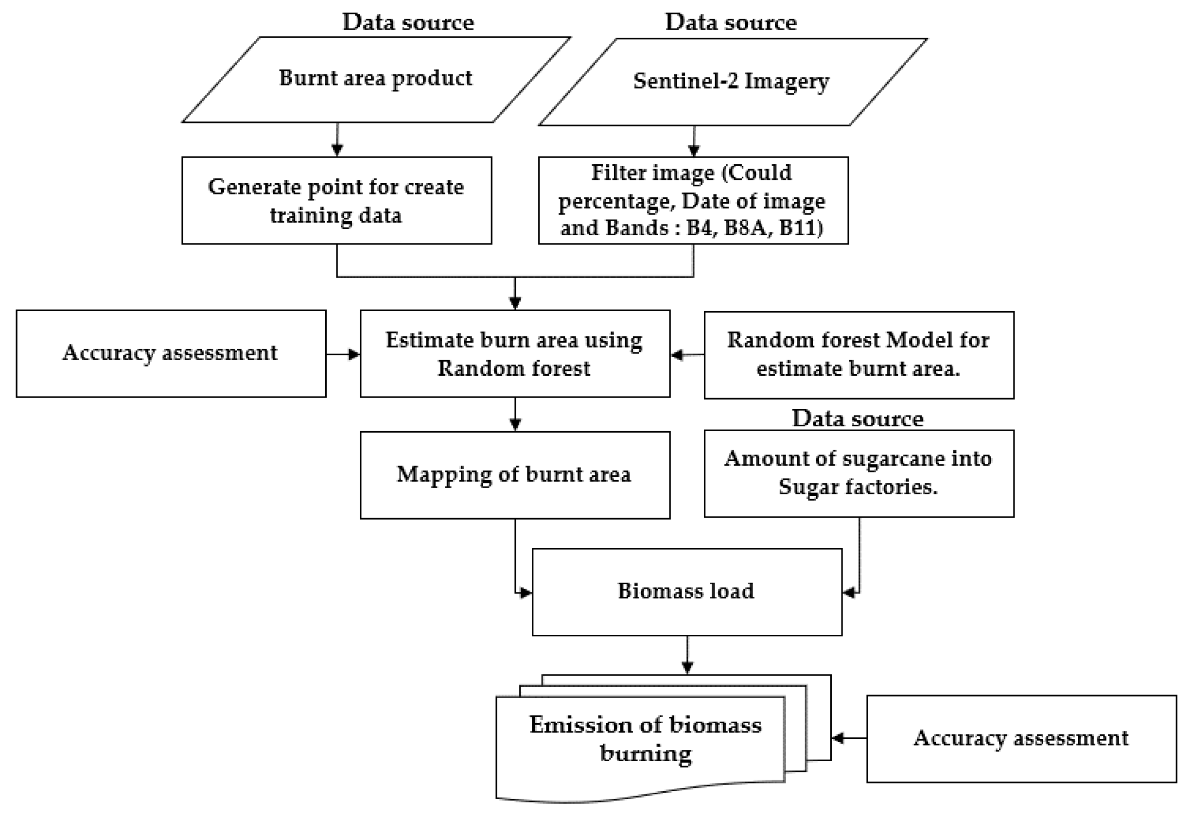
2.1. Conceptual Framework

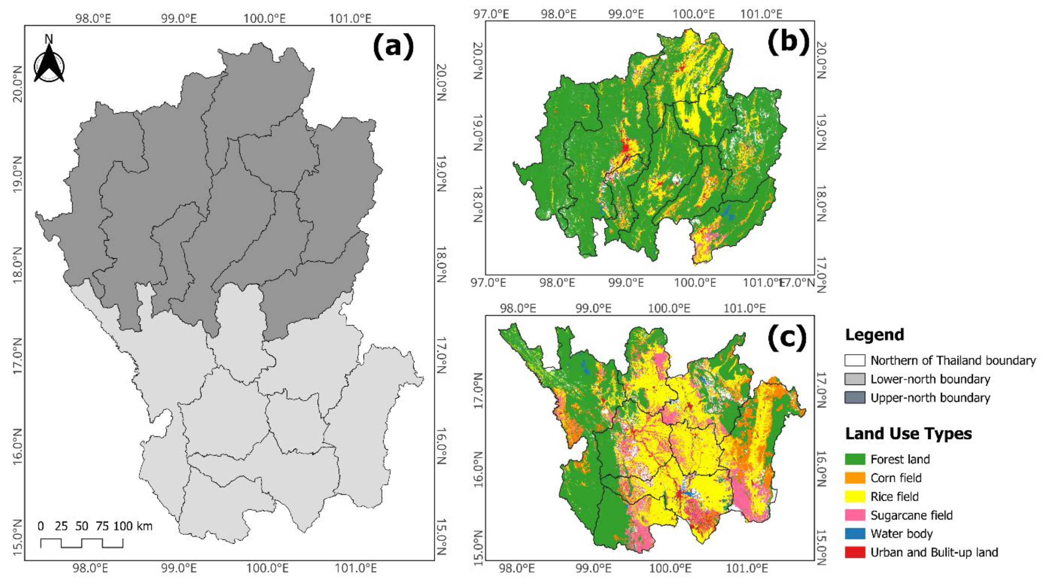
The Geo-Informatics and Space Technology Development Agency (GISTDA), a public organization, contributed Landsat-8 OLI/TRI imagery with a 30 m resolution for the burned area product or reference dataset. This dataset is the basis for burned area estimation training. The GEE platform processes using the RF algorithm. The burned area data are used to calculate air emissions using emission factors (EFs) specific to forest fires and agricultural waste residues, especially in rice, corn, and sugarcane plantations. Sugar factories are a major cause of air pollution in this region. These enterprises pollute the air by powering boilers and factories with biomass fuel (bagasse). Sugar factories’ air emissions are estimated using the Office of the Cane and Sugar Board’s (OCSB) sugarcane output data. In addition, we also used the correlation matrix, which was analyzed in open statistical software, namely jamovi version 2.3.28, to analyze the correlation between the emission inventories from our study results with the AOD data and the pollutants reported by the Sentinel-5p satellite. The correlation matrix is a commonly used statistical method that helps to evaluate the relationship between two variables. A positive correlation indicates a direct relationship between variables, while a negative correlation suggests an inverse relationship (Figure 1).

Our study utilizes two main types of datasets: data accessed through the GEE platform and data provided by government agencies in Thailand. The first type of data includes Sentinel-2 imagery, which is acquired through the Copernicus Program’s Earth observation mission and is a crucial resource for estimating open biomass emission. Additionally, AOD data are collected by the Moderate Resolution Imaging Spectroradiometer (MODIS) instrument on the Terra satellite, while the TROPOMI instrument on the Sentinel-5p satellite records NO_X and SO₂ pollutant data. The second type of data encompasses Burned reference data, which are processed using Lantsat-8 and maintained by GISTDA. This includes statistical data on the amount of sugarcane in each sugar factory, collected from the OCSB.

2.2. Study Area

The study area corresponds to northern Thailand, covering an area of around 169,644.3 km², located in Southeast Asia, with latitudes and longitudes extending from 15° N to 20° north and from 97° E to 100° east, respectively. There are 17 provinces in this region, which are classified into upper-northern and lower-northern areas [27], as shown in Figure 2. Air pollution is the main problem during the dry season in both areas, with varying sources of air pollution based on each area’s characteristics. In the upper-north region, the main areas are forest areas, covering approximately 89,902.7 km². In contrast, the lower-north region is mainly an agricultural area since most of the land is low-lying. This area is primarily dedicated to rice plantations as the main economic crop, covering an approximate area of 27,934.2 km², followed by corn and sugarcane plantations, which cover approximately 7569.9 and 3892.6 km², respectively.

2.3. Google Earth Engine Platform (GEE)

The Google Earth Engine platform (GEE) is open-source software featuring a cloud-based platform that offers convenient and efficient access to its resources. Users can work efficiently through the Internet with a web browser, eliminating the need to download software or store data locally on their computers. Instead, the GEE platform uses the service provider’s computer’s resources, streamlining the process for users. This approach allows users to process massive and ever-growing amounts of geospatial data easily, including climate and weather datasets, imagery, and geophysical datasets. Geophysical processing is implemented in programming languages such as Python and Java, and the GEE platform also provides an Application Programming Interface (API) that enables users to write commands for data processing or the creation of related applications efficiently [19,20,21,28,29,30].

2.4. Data Collection

This study used publicly available and government sources to estimate air pollutant emissions from open biomass burning. Sentinel-2 image, land use/cover, and sugarcane production data were collected. First, Sentinel-2 surface reflectance time-series pictures estimated burned areas for 2019–2021 during dry seasons on GEE. The 12-band Sentinel-2 picture collection (B1–B12) selected B4, B8A, and B11 bands with 10, 20, and 20 m resolutions. Second, the Land Development Department in Thailand provided land use and land cover data to identify spatial characteristics and pollutant sources. This study focuses on forest and agricultural regions like rice, corn, and sugarcane plantations, which are the main sources of pollution. The assessment’s burned area is characterized by land use and land cover to calculate burned biomass. Finally, 13 enterprises in the research area provided 2019–2021 sugarcane production data to sugar factories. Thailand’s OCSB provided this information. This section shows that 90% of the harvested sugarcane products in the lower-northern region is used to supply sugar manufacturing. Using bagasse as fuel in sugar factories is another major cause of air pollution in the research region [25,31,32].

2.5. Estimation of Burned Area

This study examined burned forest and agricultural land, including rice, corn, and sugarcane plantations, in dry seasons from 2019 to 2021. We evaluated this using ML on GEE. This platform provides JavaScript data processing and cloud data collection, minimizing the limits of working in wide research regions and eliminating the need to download photographs and devote storage space. Previous studies [19,20,21,28,29,30] have shown that study area limits can be overcome, allowing researchers to use vast study regions. Over the past decade, many studies have been conducted on estimating burned areas to develop approaches to reduce working time. Among these approaches, the ML approach has gained considerable popularity. In previous studies assessing burned areas, the RF algorithm was used and showed high assessment accuracy [33,34,35,36,37,38]. This study employed the RF algorithm to classify burned areas in northern Thailand during the dry season between 2019 and 2021.

2.5.1. Random Forest (RF)

The Random Forest (RF) algorithm is a data-classification algorithm based on the Decision Tree Algorithm (DT) [39]. Its principle is to divide the data into multiple trees, each with different data points and features. This diversity aims to achieve more independent trees. During the training process, each tree is trained on a random subset of variables, and features are selected randomly using random sampling with replacement. The prediction results of each tree are combined using the majority vote method, where the most frequently predicted value is chosen as the final prediction—a technique known as Bagging (Bootstrap Aggregation). The researcher analyzed the data using the Random Forest algorithm, which can be accessed from Data Collection in the GEE platform. The algorithm was configured with 1000 decision trees, each with a maximum of 1000 branches [40,41].

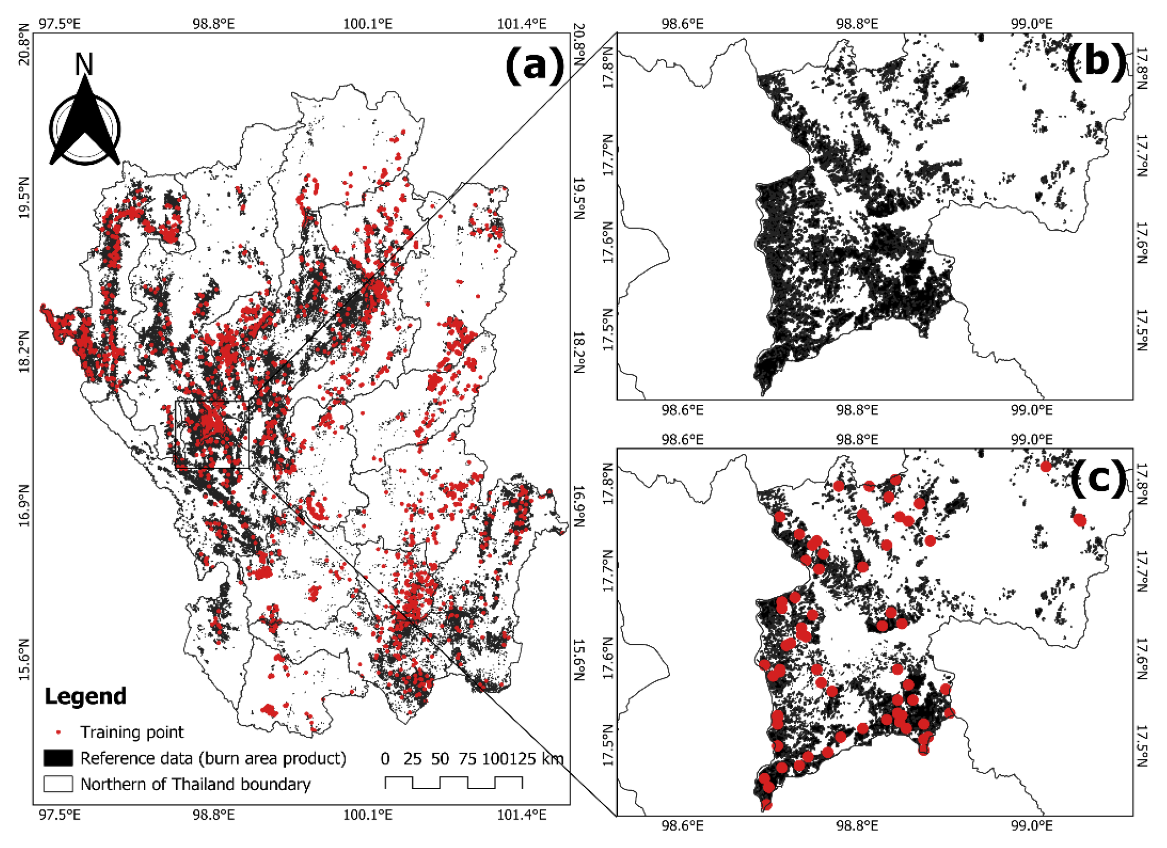
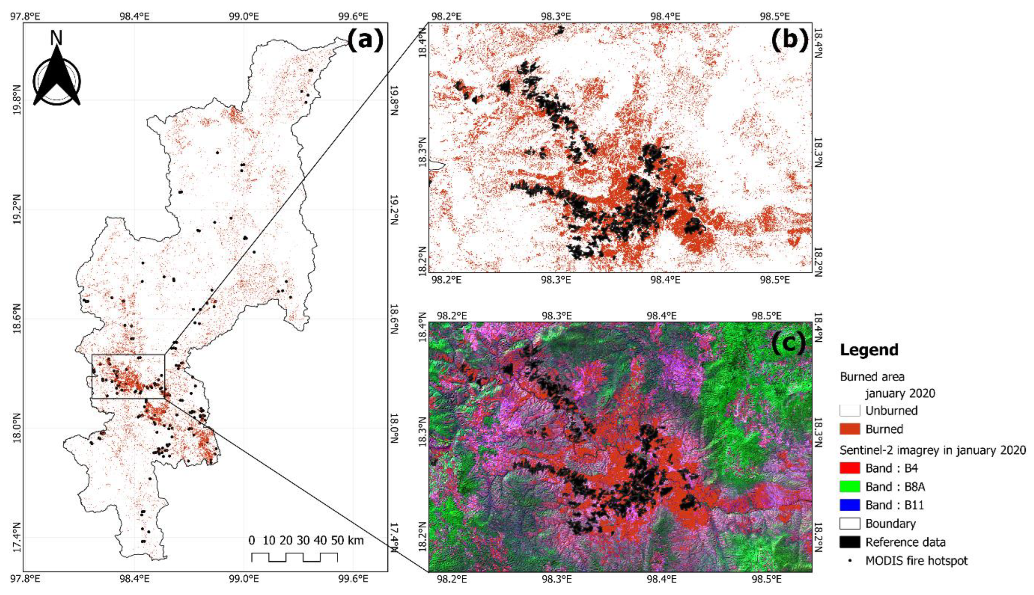
2.5.2. Burned Reference Data

The burned area product during the haze episode for the years 2019–2021 was reported by the GISTDA in Thailand. These data were obtained by processing Landsat-8 images with a spatial resolution of 60 m. The reference data were used to create training data for estimating the burned area and assessing the accuracy of the results. To generate the training data from the reference data, the data in the polygon format were processed using the Random Points tool in Geographic Information System (GIS) software (ArcMap) version 10.8. For generated training data from the references data, the data in the format of polygons were processed using the Random Points tool in ArcMap and a combination of red, near-infrared (NIR), and shortwave infrared (SWIR) bands of Sentinel-2 in the GEE platform. Moreover, 6800 training data points were classified, with 100 points in each province, and they were used to train and test the model using the RF algorithm in the GEE platform. It is important to note that the training data were created from the reference data in 2021 and used to estimate the burned area for 2019–2020 (Figure 3a–c). This is due to the limitation of the dataset reported by GISTDA, which does not cover the lower part of the study area for 2019–2020.

2.5.3. Accuracy Assessment

We calculated Cohen’s kappa coefficient [42]. This was performed based on the number of reference points in the study area. Cohen’s kappa coefficient ($\widehat{k}$) can be calculated using the following equation:

$$\widehat{k}=\frac{p_o-p_e}{1-p_e}$$

(1)

where $p_o$ is the relative observed agreement among raters, and $p_e$ is the hypothetical probability of chance agreement. Cohen’s kappa coefficient can be interpreted in

Table 1. Cohen’s Kappa coefficient.

$\mathbf{Cohen}’\mathbf{s} \mathbf{Kappa} (\widehat{\mathit{k}}$) Value	$\mathbf{Interpretation} \mathbf{of} \mathbf{the} \mathbf{Cohen}\text{’}\mathbf{s} \mathbf{Kappa} (\widehat{\mathit{k}}$)
0	No agreement
0.10–0.20	Slight agreement
0.21–0.40	Fair agreement
0.41–0.60	Moderate agreement
0.61–0.80	Substantial agreement
0.81–0.99	Near-perfect agreement
1	Perfect agreement

, where the kappa value ranges from 0 to 1. A value of 1 indicates perfect agreement, while values less than 1 indicate less than perfect agreement, as shown in Table 1 [42].

2.6. Estimation of Air Emission from Biomass Burning

The assessment of emissions from forest fires and agriculture residues consists of two steps. Firstly, the equation for annual emissions is calculated by multiplying the activity data by the emission factor. The emission estimation was performed by following the Atmospheric Brown Cloud (ABC) Emission Inventory Manual, an approach developed by the Asian Institute of Technology, Thailand [43]. Secondly, the equation for estimating the activity rate represents the relationship between the burnt area and the combustion process.

2.6.1. Forest Fire

The emissions of air pollutants emitted from forest fires were calculated using the equation developed by Giglio. et al. (2006) [44]. The annual emission equation is calculated by multiplying the amount of burning biomass obtained from the burned area by the mass of emissions emitted per biomass combusted. The equation provided is shown below:

$$E{M}_{i,j}={\displaystyle \sum }_j{M}_j\times E{F}_{i,j}$$

(2)

where $E{M}_{i,j}$ is the emission of pollutant (i) from area (j), and $M_j$ is the amount of burned biomass on area (j). $E{F}_{i,j}$ is the emission factor of pollutant (i) from area (j) (g/kg of dry matter), which are the data from the literature review, as shown in Table 2. $M_j$ for the forest fire was calculated from the following equation:

$$M=A\times B\times C$$

(3)

where A is the burned area (km²); B is the biomass density in the forest area (kg_{dry mass}/km²); and C is the burning efficiency, as shown in Table 3.

2.6.2. Agriculture Residues

The amount of air pollutants emitted from agricultural waste residues was assessed using the same equation as that for forest fires (Equation (2)), developed by Giglio et al. (2006) [44]. However, the evaluation process differed in estimating the amount of burned biomass (M), which was calculated using the equation developed by the Revised 1996 IPCC Guidelines for National Greenhouse Gas Inventories [45]. This was calculated by the following equation:

$$M=BA\times BL\times CC$$

(4)

where BA is the burnt area, BL is the biomass load (tons of dry matter/ha), and CC is the fraction of the mass combusted by fire. The BL and CC are shown in Table 3.

Table 2. Summary of emission factors for each pollutant (unit: g/kg_{dry mass}).

Type	Pollutants
	PM1	PM2.5	PM10	NOX	SO2	CO	BC	OC
Forest	0.74 a	3.4 a	7.95 a	2.55 b	0.40 b	93 b	0.52 b	4.71 b
Total Rice	0.48 a	2.13 a	5.5 a	0.21 c	1.53 c	25.80 c	0.58 f	3.5 f
Corn	0.86 a	4.71 a	7.69 a	0.07 c	1.50 c	29.79 c	0.75 f	3.71 f
Sugarcane	0.59 a	2.04 a	8.07 a	1.5 g	0.53 g	40.1 g	0.73 g	1.25 g
Bagasse	1.06 a	5 a	9.2 a	3.3 h	0.76 h	8.14 h	-	-

Source: ^a Samae et al., 2020 [8]; ^b Junpen et al., 2020 [46]; ^c Punsompong, 2016 [47]; ^f Zhang et al., 2018 [48]; ^g Junpen et al., 2020 [26] and ^h Sahu et al., 2015 [49].

Table 2. Summary of emission factors for each pollutant (unit: g/kg_{dry mass}).

Type	Pollutants
	PM1	PM2.5	PM10	NOX	SO2	CO	BC	OC
Forest	0.74 a	3.4 a	7.95 a	2.55 b	0.40 b	93 b	0.52 b	4.71 b
Total Rice	0.48 a	2.13 a	5.5 a	0.21 c	1.53 c	25.80 c	0.58 f	3.5 f
Corn	0.86 a	4.71 a	7.69 a	0.07 c	1.50 c	29.79 c	0.75 f	3.71 f
Sugarcane	0.59 a	2.04 a	8.07 a	1.5 g	0.53 g	40.1 g	0.73 g	1.25 g
Bagasse	1.06 a	5 a	9.2 a	3.3 h	0.76 h	8.14 h	-	-

Source: ^a Samae et al., 2020 [8]; ^b Junpen et al., 2020 [46]; ^c Punsompong, 2016 [47]; ^f Zhang et al., 2018 [48]; ^g Junpen et al., 2020 [26] and ^h Sahu et al., 2015 [49].

Table 3. Summary of the parameters used for the estimated emission inventory.

Parameters	Crops
	Total Rice	Corn	Sugarcane	Forest
Burn Efficiency Ratio (nj)	0.95 a	0.92 a	0.95 a	0.79 b
Biomass Density (g/m2) (B)	-	-	-	3.76 × 105 a
Biomass Load (BL) (t/ha)	7.62 c	5.26 d	9.40 e	-
Combustion Completeness (CC)	0.34 c	0.85 d	0.64 e	-

Source: ^a Sahu et al., (2015) [49]; ^b Kanabkeaw et al., (2010) [50]; ^c Cheewaphongphan et al., (2013) [51]; ^d Kanokkanjana et al., (2011) [52] and ^e Sornpoon et al., (2014) [53].

Table 3. Summary of the parameters used for the estimated emission inventory.

Parameters	Crops
	Total Rice	Corn	Sugarcane	Forest
Burn Efficiency Ratio (nj)	0.95 a	0.92 a	0.95 a	0.79 b
Biomass Density (g/m2) (B)	-	-	-	3.76 × 105 a
Biomass Load (BL) (t/ha)	7.62 c	5.26 d	9.40 e	-
Combustion Completeness (CC)	0.34 c	0.85 d	0.64 e	-

Source: ^a Sahu et al., (2015) [49]; ^b Kanabkeaw et al., (2010) [50]; ^c Cheewaphongphan et al., (2013) [51]; ^d Kanokkanjana et al., (2011) [52] and ^e Sornpoon et al., (2014) [53].

2.6.3. Agro-Industries

Agro-industries, notably sugar plants, contribute to pollution by burning biomass. Thailand’s second-largest sugarcane cultivation area is 169,644.3 km². Fresh and charred sugarcane exist. Sugar plants create power for boilers and other industries with harvested sugarcane. Bagasse, a byproduct of juice extraction, can be transformed into renewable energy for production heating [23,24]. Sugarcane bagasse is used to generate steam in the boiler furnace after juice extraction for manufacturing. Industrial air pollutants might also be released during this process, affecting air quality. There are 13 sugar factories in the study area, and they are mainly allocated in the lower north of the region, which supervises the OCSB in Thailand. The amount of emissions from sugar factories was proposed by an estimation method developed by Sahu et al. (2015) [49], as detailed below:

$$T{O}_j={\displaystyle \sum }_i^{a}F{U}_i\times E{F}_j$$

(5)

where TO_j is the total emission for a specific pollutant (j), FU_i is the bagasse amount for specific sugar factories (i), and EF_j is an emission factor of different pollutants emitted from boilers in sugar factories, as shown in Table 2.

3. Results

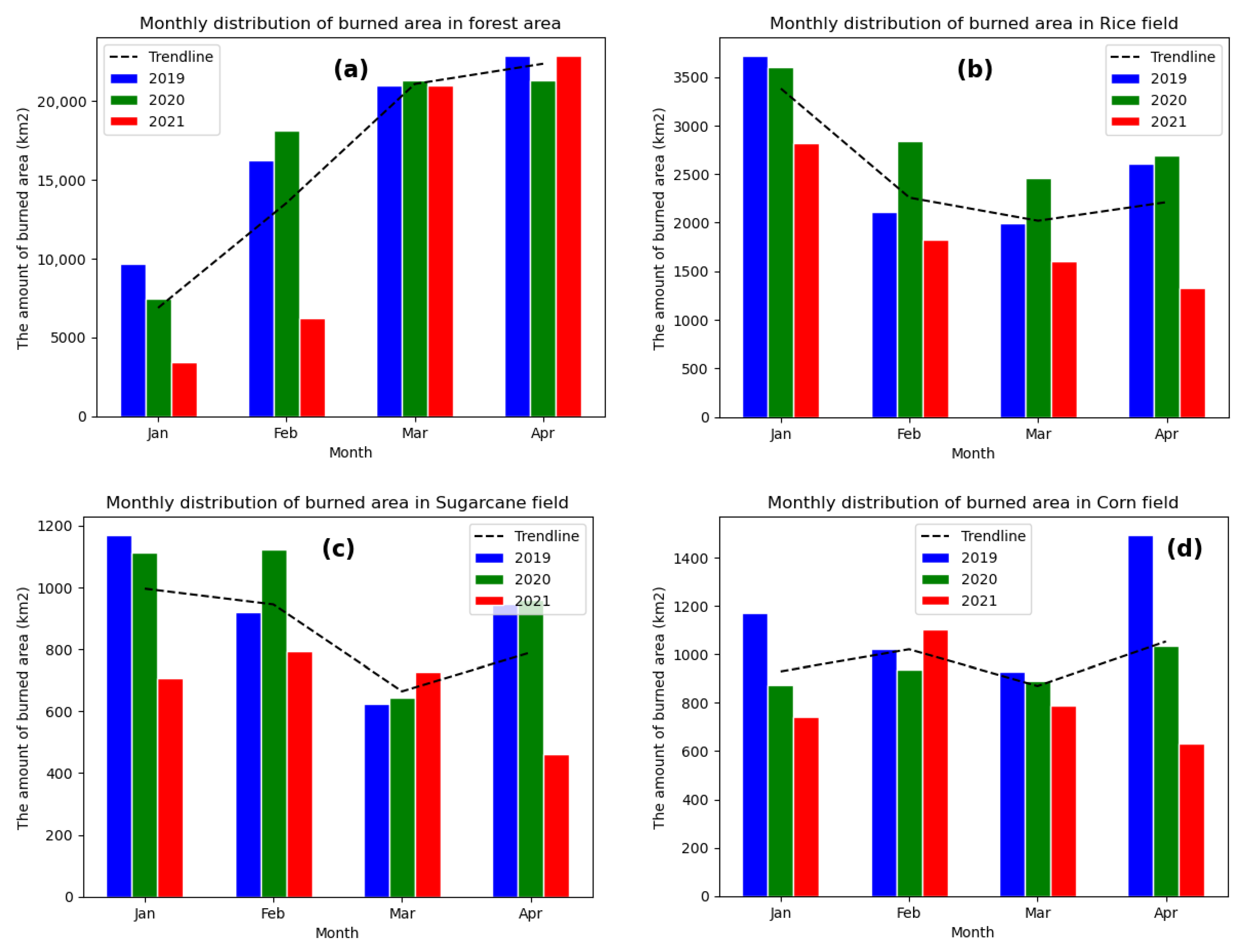
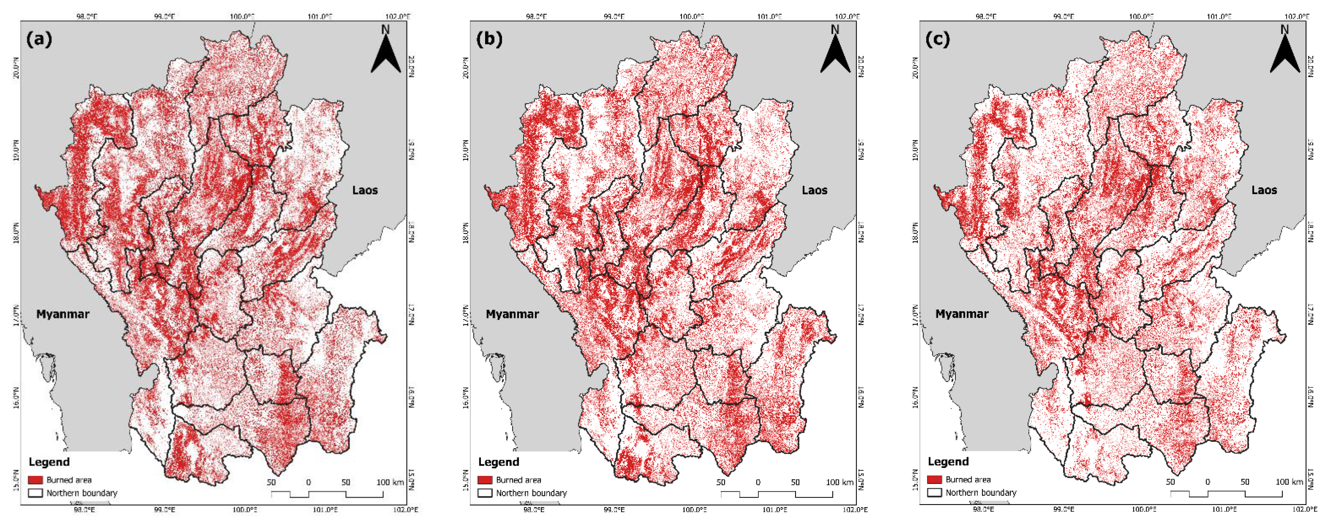
3.1. The Spatial Distribution of Burned Area in Northern, Thailand

The total burned area over the dry seasons from 2019 to 2021 amounted to roughly 153,735.2 km². In 2019, the burned area peaked at 88,465.3 km², accounting for 51.4% of the study area. Of this, 69,753.9 km² (78.8%) was from forest fires, while 18,711.4 km² (21.2%) was from agricultural areas. In 2020, the following areas were discovered: 87,332.4 km2 or 50.8% of the study area was affected by forest fires, with 68,166.4 km² or 78.1% of the forest area and 19,165.4 km² or 21.9% of the agricultural area being affected. In 2021, the burned area was the smallest, at 63,500.2 km², which accounted for 33.8% of the study area. Of this burned area, 69,753.9 km² (82.4%) originated from forest fires, while 13,534.0 km² (27.6%) originated from agricultural regions. The burned area is displayed in

Table 4. The total burnt area that was estimated by Sentinel-2 during the haze episode.

Year	Month	The Burnt Area from Assessment (km2)				Total
		Forest	Rice	Corn	Sugarcane
2019	January	9688.5	3719.8	1173.1	1169.9	15,751.3
	February	16,233.3	2106.1	1022.4	920.9	20,282.7
	March	20,955.3	1993.6	929.6	623.3	24,501.8
	April	22,876.9	2611.7	1495.4	945.6	27,929.6
	Total	69,753.9	10,431.2	4620.5	3659.7	88,465.3
2020	January	7484.9	3600.4	874.7	1111.3	13,071.4
	February	18,089.7	2836.6	937.6	1120.8	22,984.7
	March	21,295.0	2460.7	890.8	643.5	25,289.9
	April	21,296.8	2694.4	1034.0	961.2	25,986.4
	Total	68,166.4	11,592.1	3737.1	3836.8	87,332.4
2021	January	3434.7	2819.5	742.2	705.6	7701.9
	February	6233.3	1829.4	1103.4	792.6	9958.8
	March	20,955.3	1605.2	788.4	725.4	24,074.2
	April	22,876.9	1328.6	631.4	462.2	25,299.1
	Total	63,500.2	7582.8	3265.4	2685.8	77,034.1

. Figure 4 shows the monthly distribution of burned areas during dry seasons in northern Thailand. It was found that forest fires had been occurring since January, and the peak period was in March–April, as shown in Figure 4a. On the other hand, the burning of agricultural waste is indicated by an uncertain burning period due to variations in planting and harvesting schedules. Especially in the rice plantation, as shown in Figure 4b, the burning area was particularly high in January, which coincides with the harvest seasons, which peaks from November. The burning of corn and sugarcane residues in the field indicated a similar time series, as shown in Figure 4c,d. The burned area remained relatively constant over 5 months (December–April), with the peak harvesting period for corn occurring from October to December, aligning with the cold dry season. Similarly, in sugarcane plantations, which can be harvested during the cold dry season, the peak harvest period for crushing seasons was from January to April [46].

The spatial distribution of burned areas shows that forested regions have the highest density of burned areas, particularly in provinces such as Mae Hong Son, Tak, Chiang Rai, and Chiang Mai (Figure 5). This observation aligns with the geological characteristics of the study area, which mainly consists of forest areas. Additionally, certain types of agriculture, such as corn plantations, are practiced within this region. There is a growing trend of expanding plantation areas, invading further into forest areas. This expansion is driven by the favorable characteristics of corn, which is relatively easy to grow and does not require substantial amounts of water.

3.2. The Accuracy Assessment of Burned Area

The burned area assessment results obtained from the RF algorithm were validated with the burned area estimation dataset derived from Landsat-8 OLI/TRI reported by GISTDA (

Table 5. Confusion matrix and performance metrics of the assessment of the burned area in Chiang Mai, Thailand.

Confusion Matrix	Predicted		Performance Metrics
	Not Burned (TN)	Burned (FP)	Accuracy	Precision	Recall	F1 Score
Actual
Not burned	167	6	95.14%	91.89%	91.89%	87.48%
burned	6	68	95.14%	96.53%	96.53%	96.53%
Overall accuracy (%)	95.14%
Kappa coefficient	0.8842

). The validation process yielded kappa coefficients of 0.83, 0.82, and 0.83, respectively, over the 3 years, indicating good consistency between the assessment and the dataset. The overall accuracy of the validation was found to be 85%. The evaluation also utilizes hot spots obtained from MODIS satellite measurements that coincide with the same period. Moreover, it incorporates line considerations through false color combinations of Sentinel-2 satellite imagery in the bands B4, B8A, and B11, where the burned area is importantly highlighted. Figure 6 shows an example of a map of the burned area estimated by the RF algorithm in Chiang Mai overlaid with training data and Sentinel-2 imagery (B4, B8A, and B11).

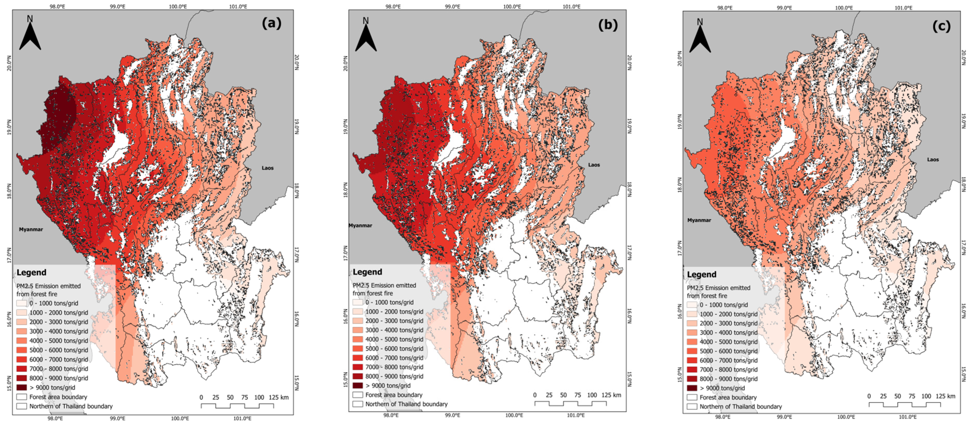
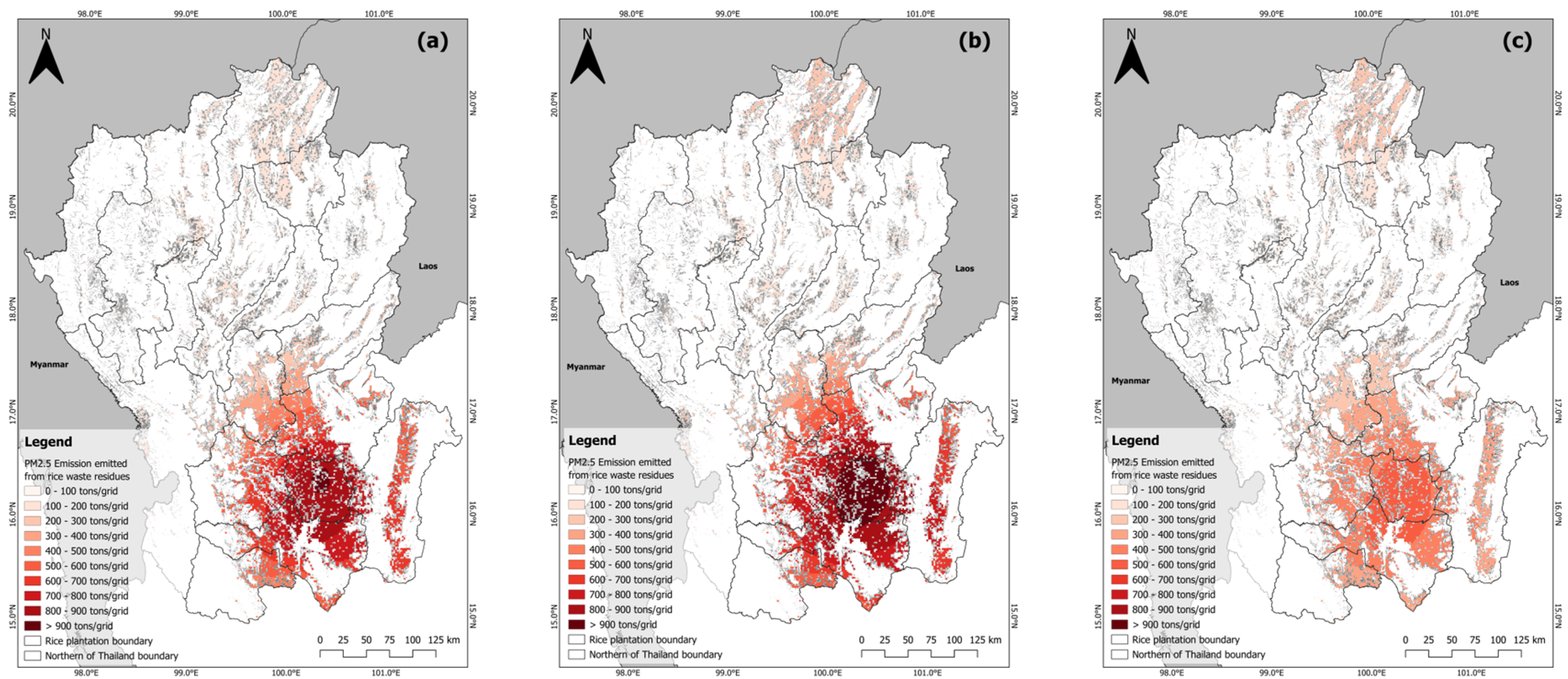
3.3. Total Emissions from Open Biomass Burning

In assessing the air emissions from open biomass burning, the total emissions from agricultural waste residues and forest fires during 2019–2021 were estimated using Equation (1) for the forest area and Equation (2) for agricultural residues. The emission factors (EFs) and parameters reserved in the calculations are detailed in Table 1 and Table 2, and the amount of air emissions is presented in

Table 6. The emissions from biomass burning.

Year	Type	Type of Pollutants (tons/year)
		PM1	PM2.5	PM10	NOX	SO2	BC	OC
2019	Forest fire	15,332.6	70,447.0	164,721.7	52,835.3	8287.9	10,774.3	97,589.8
	Total rice	1297.2	5756.4	14,863.8	567.5	4134.8	1567.5	9458.8
	Corn	1776.6	9730.0	15,886.1	144.6	3098.7	1549.4	7664.2
	Sugarcane	1299.0	4491.4	17,701.4	3302.5	1166.9	1607.2	2752.1
	All Type	19,705.4	90,424.7	213,173.0	56,849.9	16,688.3	15,498.3	117,464.9
2020	Forest fire	14,983.6	68,843.7	160,972.8	51,632.8	8099.3	10,529.0	95,368.8
	Total rice	1441.6	6397.0	16,518.0	630.7	4595.0	1741.9	10,511.5
	Corn	1436.9	7869.6	12,848.7	116.9	2506.3	1253.1	6198.8
	Sugarcane	1361.9	4708.8	18,558.1	3462.3	1223.4	1685.0	2885.3
	All Type	19,224.0	87,819.1	208,897.7	55,842.8	16,423.9	15,209.1	114,964.3
2021	Forest fire	9796.3	45,010.2	105,244.3	33,757.6	5295.3	6883.9	62,352.3
	Total rice	943.0	4184.5	10,805.0	412.6	3005.8	1139.4	6875.9
	Corn	1255.6	6876.4	11,227.0	102.2	2189.9	1095.0	5416.4
	Sugarcane	953.3	3296.2	12,990.9	2423.7	856.4	1179.5	2019.7
	All Type	12,948.2	59,367.2	140,267.2	36,696.0	11,347.4	10,297.8	76,664.4
	All	51,877.5	237,611.0	562,337.8	149,388.7	44,459.6	41,005.2	309,093.6

. The findings indicate that forest fires during 2019–2021 emitted air pollutants totaling 3926.0 tons of PM₁, 17,886.0 tons of PM_2.5, 3084.5 tons of NO_X, and 5401.3 tons of SO₂. Notably, the highest emissions occurred in 2019, with 736.8 tons of PM₁, 3372.3 tons of PM_2.5, 564.2 tons of NO_X, and 999.8 tons of SO₂. Conversely, the lowest air emissions were reported in 2021, amounting to 507.7 tons of PM₁, 2320.3 tons of PM_2.5, 397.9 tons of NO_X, and 709.3 tons of SO₂. Analyzing the trend of air emissions reveals a correlation with the utilization of agricultural areas, with higher emissions observed in sugarcane plantations, followed by corn plantations, forest areas, and rice plantations, respectively. The assessment indicates an unstable emission trend between 2019 and 2021, characterized by a peak in 2019 followed by a decline in 2020–2021. One contributing factor to this instability is climate change, particularly the La Niña Phenomenon [54,55,56]. During the La Niña years of 2020 and 2021, a significant increase in precipitation was observed during typically dry seasons, leading to a deviation from customary fuel moisture levels. Furthermore, 2020 witnessed the global spread of the COVID-19 pandemic, impacting people’s lives and directly affecting the economy, including the demand for agricultural products [57,58,59,60,61]. This factor also contributed to the observed fluctuations in air emissions during this period.

The spatial distribution of PM_2.5 emissions from open biomass burning (grid size 1 km × 1 km) is shown in Figure 7, Figure 8, Figure 9 and Figure 10. Figure 7a–c shows that the upper-north region emitted the highest PM_2.5 emissions from forest fires, primarily due to its extensive forest cover, encompassing approximately 64.9% of the upper-north area. This correlation between high emissions and significant forest cover is notable in provinces such as Mae Hong Son, Chiang Mai, and Tak, where the distribution of PM_2.5 can be found at concentrations ranging from 5000 to 6000 tons/grids. Conversely, the lower-north region had heightened PM_2.5 emissions from burning crop residue; notably, the burning of rice waste, particularly in Sukhothai, Kamphaeng Phet, Phitsanulok, and Nakhon Sawan, contributed to a higher density of PM_2.5 emissions, with the year 2020 featuring the highest density, with PM_2.5 emissions reaching approximately 600–700 tons/grids (Figure 8a,b). These provinces, characterized by lowland areas conducive to rice cultivation, have rice as a primary economic crop. Similarly, the burning of sugarcane wastes indicates a high density in provinces such as Nakhon Sawan, Kamphaeng Phet, Uthai Thani, and Phetchabun, with Phetchabun showing the highest density at approximately 1000–1200 tons/grids (Figure 9a–c). Notably, over 90% of harvested sugarcane products are sent to sugar factories—a trend attributed to the proximity of sugarcane plantations to these factories, influencing the burning activities in sugarcane plantations to meet factory demands. Furthermore, PM_2.5 emissions from corn waste residues are notably higher in provinces such as Nan, Chiang Rai, and Lampang compared to other regions, as evidenced in Figure 10a–c. The upper-northern region has a significant presence of corn residues, extending into areas without extensive irrigation systems, as corn cultivation thrives in these regions due to its ability to grow with minimal water requirements. Although the density of burning corn waste is lower than rice and sugarcane waste residues, it continuously impacts regional air quality.

3.4. Total Emissions from Agro-Industries (Sugar Factory)

Figure 11 shows the sugarcane production and bagasse use in the sugar factories across the study area. This includes 13 sugar factories, with Kamphaeng Phet having the highest number of sugar factories, with 3 factories, followed by Nakhon Sawan, Phetchabun, and Uthai Thani provinces, with 2 factories. The raw materials for these sugar factories are sourced during the annual crushing seasons, covering approximately five months from December to April. Throughout the years 2019–2021, Kamphaeng Phet recorded the highest sugarcane production transported into sugar factories, reaching around 7705,759.0 tons in 2019, followed by 4907,854.9 tons in 2020 and 4531,978.7 tons in 2021. It is worth noting that the quantity of sugarcane production utilized by each factory varies based on the number of industries in the area and their registered capacity. Moreover, the procurement of sugarcane production extends to various regions surrounding the sugar factories, contributing to the diverse sourcing patterns observed in these facilities.

Table 7. The emissions from agro-industries in sugar factories.

Province	Emission of Pollutants (tons/year)
	2019			2020			2021
	SO2	NOX	PM2.5	SO2	NOX	PM2.5	SO2	NOX	PM2.5
Nakhon Sawan (2)	27.1	117.7	178.3	12.6	54.9	83.1	18.5	80.4	121.8
Uttaradit (1)	7.5	32.6	49.4	6.1	26.5	40.1	4.8	20.8	31.5
Phetchabun (2)	24.2	105.2	159.3	12.1	52.6	79.6	14.1	61.2	92.7
Kamphaeng Phet (3)	328.0	1424.0	2157.6	208.9	907.0	1374.2	192.9	837.5	1269.0
Sukhothai (1)	77.3	335.5	508.3	50.2	217.9	330.2	39.9	173.1	262.3
Phitsanulok (1)	12.0	52.0	78.8	7.1	30.9	46.8	5.9	25.7	39.0
Uthai Thani (2)	71.9	312.1	472.9	34.7	150.8	228.6	34.8	150.9	228.7
Total	547.9	2379.1	3604.8	331.8	1440.5	2182.6	310.8	1349.7	2045.0

presents the air emissions from sugar factories utilizing bagasse for power generation in their production processes, estimating NO_X, SO₂, and PM_2.5 emissions for the production years of 2019–2021. The results showed that PM_2.5 emissions peaked in 2019 at 3604.8 tons, followed by NO_X at 2379.1 tons and SO₂ at 547.9 tons. In 2020, PM_2.5 emissions were 2182.6 tons, accompanied by NO_X at 1440.5 tons and SO₂ at 331.8 tons. This trend continued in 2021, with PM_2.5 emissions at 2045.0 tons, NO_X at 1349.7 tons, and SO₂ at 310.8 tons. Moreover, the highest air emissions were observed in Kamphaeng Phet, followed by Sukhothai, Uthai Thani, and Nakhon Sawan. Notably, the air emissions from each sugar factory are contingent on the number of industries in the area, including the production capacity of the factories, influencing their ability to process larger quantities of sugarcane compared to industries in other provinces. Finally, the spatial distribution of PM_2.5 emissions from sugar factories in each province is shown in Figure 12.

3.5. Correlation between Emission Inventory, AOD, and Air Monitoring Pollutant

3.5.1. Particulate Matter

Figure 13 shows the amount of monthly PM_2.5 emissions from forest fire and agriculture waste residues with monthly AOD at the Chiang Mai Government Center (Chiang Mai-1) and the Yupparaj Wittayalai School (Chiang Mai-2), which are data at the location of the PCD air-monitoring stations. The AOD is a measure that indicates the relationship between the portion of particles measured vertically above the ground and the number of particles recorded at the observation point on the ground. It is commonly used to predict and monitor the PM_2.5 situation because it estimates the average value of PM_2.5 covering all areas throughout the country. We used the AOD value obtained from the MODIS satellite observation. This was because the air monitoring of pollutants reported by PCD stations was unavailable during the study period.

In Figure 13a–c the data indicate that in Chiang Mai-1, forest fires are the primary source of air pollution. This was evident from March to April when there was an increase in the PM_2.5 emission from forest fires, and the AOD levels were higher during the same period. However, when comparing with Chiang Mai-2, as shown in Figure 14a–c, the trend is similar, but the AOD values are higher than in Chiang Mai-1. This could be attributed to the location, particularly within the economic zone, mainly due to motor vehicles.

Table 8. Correlation matrix between the AOD and open biomass burning emissions at Chiang Mai-1 in 2019.

Variables	AOD	Open Biomass Burning Emissions
		Forest Fire	Corn Waste	Rice Waste	Sugarcane Waste	Total Biomass Emission
AOD	−1
Forest fire	0.906	−1
Corn waste	−0.320	−0.689	−1
Rice waste	−0.212	−0.088	−0.246	−1
Sugarcane waste	0.039	−0.385	0.934	−0.322	−1
Total biomass emissions	0.994	0.941	−0.410	−0.140	−0.057	−1

,

Table 9. Correlation matrix between the AOD and open biomass burning emissions at Chiang Mai-1 in 2020.

Variables	AOD	Open Biomass Burning Emissions
		Forest Fire	Corn Waste	Rice Waste	Sugarcane Waste	Total Biomass Emission
AOD	−1
Forest fire	0.886	−1
Corn waste	−0.841	−0.662	−1
Rice waste	−0.904	−0.624	0.927	−1
Sugarcane waste	−0.868	−0.547	0.747	0.941	−1
Total biomass emissions	0.811	0.986	−0.531	−0.495	−0.440	−1

and

Table 10. Correlation matrix between the AOD and open biomass burning emissions at Chiang Mai-1 in 2021.

Variables	AOD	Open Biomass Burning Emissions
		Forest Fire	Corn Waste	Rice Waste	Sugarcane Waste	Total Biomass Emission
AOD	−1
Forest fire	0.857	−1
Corn waste	0.240	0.705	−1
Rice waste	−0.472	0.048	0.729	−1
Sugarcane waste	0.270	0.653	0.821	0.639	−1
Total biomass emissions	0.756	0.985	0.816	0.216	0.734	−1

show a correlation matrix between the average PM_2.5 emissions and the AOD value at Chiang Mai-1 in 2019–2021; mainly, in 2019, the emissions from forest fires and total biomass emissions had a direct impact on the AOD value and indicated the highest correlation during the three years, with values of 0.81 and 0.99 in 2020 and 2019, respectively, as shown in Table 8 and Table 9. On the other hand, in Chiang Mai-1, the emissions from burning rice waste and sugarcane waste in the field showed an inverse relationship with the AOD value. Thus, the emissions from both activities did not directly impact the AOD value. One of the reasons for this is the land use and land cover in Chiang Mai province, where there is limited space for both types of agriculture due to most of the area being forests. Despite this, there is a concentrated cultivation density for both types of agriculture in the lower-northern region. However, the burning incidents often occur at times that do not align with periods of air pollution issues in the area.

Moreover, the density of both types of agriculture is concentrated in the lower-northern region. However, the agricultural waste residues that occur do not correspond to periods of air pollution or dry seasons, especially in the case of sugarcane. Sugarcane is often harvested, including being burned for harvesting production before the crushing seasons, typically from December to April [25,32]. This is similar to the burning in rice waste fields, where the burning is usually at its peak in November, known as in-season rice. The relationship between the burning of agricultural waste in fields, which has less impact on AOD values than forest fires, is similar to the pattern in another province in northern Thailand.

3.5.2. NO_X and SO₂

This section shows the correlation between the amount of air emissions and air pollutant data from Sentinel-5p because the concentration of air pollutants reported by the PCD in Thailand is not available during the study period. Thus, the air monitoring data from the Sentinel-5p are used instead of the data from the PCD. Furthermore, Sentinel-5p is one of the satellites that was improved for monitoring and reporting the concentration of air pollutants from the Tropospheric Monitoring Instrument (TROPOMI) sensor. Moreover, data from Sentinel-5p are reported daily, ensuring the information is highly efficient and up-to-date with the air pollution situation.

Table 11. Correlation matrix between the AOD and open biomass burning emissions at Nakhon Sawan in 2019.

Variables	Sentinel-5p		Open Biomass Burning Emissions
	SO2	NO2	Forest Fire	Corn Waste	Rice Waste	Sugarcane Waste	Factories	Total
SO2 (Sentinel-5p)	−1
NO2 (Sentinel-5p)	−0.816	−1
Forest fire	−0.206	0.582	−1
Corn waste	−0.507	0.028	−0.737	−1
Rice waste	0.057	−0.455	−0.050	0.059	−1
Sugarcane waste	−0.160	−0.041	−0.807	0.793	−0.463	−1
Factories	0.545	−0.281	0.616	−0.896	0.386	−0.914	−1
Total	0.489	−0.526	0.304	−0.562	0.778	−0.808	0.870	−1

,

Table 12. Correlation matrix between the AOD and open biomass burning emissions at Nakhon Sawan in 2020.

Variables	Sentinel-5p		Open Biomass Burning Emissions
	SO2	NO2	Forest Fire	Corn Waste	Rice Waste	Sugarcane Waste	Factories	Total
SO2 (Sentinel-5p)	−1
NO2 (Sentinel-5p)	−0.236	−1
Forest fire	0.115	0.099	−1
Corn waste	0.426	0.641	−0.331	−1
Rice waste	−0.088	−0.937	0.000	−0.858	−1
Sugarcane waste	0.597	0.636	0.109	0.896	−0.851	−1
Factories	0.069	−0.947	−0.391	−0.566	0.899	−0.707	−1
Total	0.354	−0.910	−0.454	−0.308	0.752	−0.444	0.947	−1

and

Table 13. Correlation matrix between the AOD and open biomass burning emissions at Nakhon Sawan in 2021.

Variables	Sentinel-5p		Open Biomass Burning Emissions
	SO2	NO2	Forest Fire	Corn Waste	Rice Waste	Sugarcane Waste	Factories	Total
SO2 (Sentinel-5p)	−1
NO2 (Sentinel-5p)	−0.769	−1
Forest fire	0.531	0.077	−1
Corn waste	−0.149	−0.200	−0.774	−1
Rice waste	−0.299	−0.325	−0.967	0.811	−1
Sugarcane waste	−0.702	0.750	−0.359	0.484	0.174	−1
Factories	0.474	−0.290	0.667	−0.877	−0.589	−0.846	−1
Total	0.345	−0.120	0.698	−0.944	−0.662	−0.742	0.985	−1

show the correlation between the monthly average NO₂ and SO₂ reported by Sentinel-5p at the PCD air monitoring stations in Nakhon Sawan provinces and emissions from agricultural waste residues, forest fires, total biomass emissions, and sugar factories. The correlation matrix between SO₂ and total biomass emissions indicated a very weak correlation, with values of 0.49 in 2019, 0.35 in 2020, and 0.34 in 2021, respectively. Furthermore, the correlation between NO₂ and biomass burning emissions is unclear, indicating an inverse correlation, with values of −0.53 in 2019, −0.91 in 2020, and −0.12 in 2021, respectively. Thus, the amount of open biomass burning and emissions from sugar factories does not directly impact SO₂ and NO₂ concentrations.

The relationship between NO_X and emission estimation is less evident than the association between particulate matter and emission estimation, which showed similar results in other provinces. This could be the case because other sources, like motor vehicles and oil-burning industries, also contribute significantly or even greater amounts [25,62,63].

4. Discussion

4.1. The Assessment of Burned Areas by Using the GEE Platform

In the estimation, the RF algorithm had the highest accuracy in assessment. This result corresponds with a study by Gholamrezaie et al. (2022) [19], which reported that the RF algorithm achieved the highest accuracy, with a kappa coefficient of 0.90 and an overall accuracy of 0.89. These results indicate that the burned area using the RF algorithm for estimation was highly accurate and reliable. Moreover, numerous previous studies estimated using the ML approach also showed that the RF algorithm has high accuracy [36,37,38,39,40,41]. Furthermore, this was observed in studies in Thailand focused on estimating using the Normalized Burn Ratio (NBR) and Difference Normalized Burn Ratio (dNBR) with satellite images [62,63,64]. Although the results showed similar accuracy, the processing steps were time-consuming and involved loading satellite images. Thus, conducting large-scale assessments, especially in regions like the northern area, can be challenging. The extent of the burned area that can be assessed aligns with the report from the government sector in Thailand. The amount of burned area in the assessment was found to be consistent with the burned area report of GISTDA for the years 2019–2021 [65,66,67], which reported that 2019 featured the greatest amount of burned area, particularly in Tak, Mae Hong Son, and Lampang provinces, with burned areas of 2480.4, 2445.4, and 1635.4 km², respectively. However, the results from GISTDA are lower than those of this study. The differences between the results are due to the spatial resolution of the satellite images used to estimate the burned area: GISTDA used at-8 imagery with a resolution of 30 m, while this study used Sentinel-2 images with a resolution of 20 m. In addition, the burned area from the MCD64A1 products was lower than the burned area estimated in the study. This difference is still caused by differences in the spatial resolution of the satellite images, in which the MCD64A1 product has a spatial resolution of 500 m.

One of the reasons for the greatest burned area in 2019 was the El Niño year, which caused lower average rainfall compared to standard years [68]. The average rainfall in 2019 was recorded at 1343.4 mm, marking it as the year with the lowest precipitation within the 5 years of 2015–2019. In addition, the average temperature in 2019 recorded an annual average of 28.1 degrees Celsius, which remained higher than the average temperature during the previous 30-year period of 1981–2010. Due to the specific meteorological characteristics experienced during that year, many burned areas resulted from open burning activities. In contrast, the years 2020 and 2021 were influenced by the La Niña phenomenon, resulting in above-average rainfall. The precipitation was recorded as 1527.3 mm and 1759.3 mm, respectively, continuously increasing throughout the period. The higher precipitation levels significantly impact the atmospheric humidity and directly influence the potential for further combustion. The increased moisture content in the air is a deterrent to combustion, thereby reducing the occurrence and extent of burning activities. Furthermore, COVID-19 developed into a global pandemic in 2020. This epidemic affected the economy, especially agricultural demand. Lockdowns and travel restrictions to contain the epidemic harmed imports and exports, especially agricultural products. Supply chain disruptions and consumer behavior shifts exacerbated agricultural sector issues that year [57,58,59,60,61].

4.2. The Emissions from Open Biomass Burning

The air emissions during the assessment were consistent with previous studies, which explain that the sources of air pollution affecting the upper north are primarily caused by forest fires. In contrast, the lower north experiences pollution originating from agricultural waste [5,46,47,48,69,70,71]. Furthermore, the direction of the increase or decrease in the emissions was consistent with studies conducted by Nuthammachot et al. (2016) [31]. These results indicate that Tak, Chiang Mai, and Mae Hong Son had the highest PM_2.5 emissions caused by forest fires. In addition, the estimated amount of emissions in this study was higher than that of Jansakoo et al. (2022) [69]. Their study reported that the amount of PM_2.5 emissions emitted from forest fires was 1029 tons/year, which is 32.3% higher than the results from this study. On the other hand, the amount of PM10 emitted was reported as 961.3 tons/year, which was 52.6% lower than the results from this study. Furthermore, the amount of emissions from agricultural residues in this study remains relatively higher compared to the previous study [69]. However, a spatial consensus indicates that rice waste residues were found to have the highest air emissions. The higher air emissions compared to the previous study can be attributed to the data used in the assessment, specifically the burned area used for calculating the amount of burned biomass. This resulted in a clear difference from previous studies, particularly in terms of air emissions from agricultural areas. Most previous studies primarily focused on estimating emissions based on the quantity of agricultural products [48,70,71]. The use of yield to calculate the amount of burned biomass is a common method for assessing air pollutant emissions in agriculture. However, it is important to note that not all agricultural waste is burned. Agricultural waste can be effectively processed and utilized for various advantageous purposes, including biomass energy production, animal feed, and fertilizer production.

The measurement of air pollutant emissions resulting from open biomass burning has emerged as a significant area of focus in environmental research, particularly in the context of incorporating satellite imagery for evaluation. This study aligns with prior research by examining the evaluation of emissions resulting from open biomass burning using the measurement of burned area. The assessment primarily relied on burned area data obtained from MODIS products, notably the MCD64A1 and MCD45A1 burned area products [5,71]. Nevertheless, the assessment indicates that the quantity of emissions was reduced compared to the findings of this study as a result of disparities in geographic resolutions. The geographic resolution of the MODIS burned area product dataset is 500 m, whereas the burned area calculated in this study, which was evaluated using Sentinel-2 satellite photos, has a greater resolution of 20 m. The study conducted by Junpen et al. (2020) [26] aimed to estimate the quantity of air pollutant emissions resulting from open biomass burning in Thailand, specifically in the Greater Mekong Subregion, during the year 2015. The findings suggest that the air emissions observed in this study remain lower compared to those reported in our study. This disparity can be attributed to the variation in geographic resolution derived from satellite imagery. In addition to the factors mentioned earlier, EFs contribute to the differences from previous studies. The availability of specific EFs for Thailand is still limited. Therefore, researchers often select values from areas like the study area, including studies conducted in countries like China and India [8,26,46,47,48,72].

4.3. The Emissions from Indoor Biomass Burning

The last point is the amount of air emissions emitted from the processing in sugar factories. The results showed that the air emissions from this assessment were lower than those in studies by Janghathaikul et al. (2005) [73], which focused on sugar factories in Nakhon Ratchasima in 2005. In their study, the annual emissions were reported as 76,634 tons of NO_X. The reported assessment in this study was highest in 2021, with 1254.21 tons of NO_X, but also lower than that in studies by Janghathaikul et al. (2005) [73], with a reduction of 98.4% of NO_X. One of the differences in the results is the location of the factories: Janghathaikul et al. (2005) [73] studied Nakhon Ratchasima, located in northeastern Thailand, the region with the most sugarcane plantations in Thailand. Furthermore, when considering PM_2.5 emissions, the highest emissions were in 2019, with 3604.79 tons/year, which was lower than that reported by Sahu et al. (2015) [49], who found that PM_2.5 emissions were 444 Gg/year—more than double the results in this study. Moreover, this difference is caused by the amount of sugarcane and bagasse used in factories. The amount of bagasse in the studies by Sahu et al. (2015) [49] was higher than in this study because of the difference in the location of the study area. Additionally, one previous study on the size of the study area affected by the air emissions from sugar factories was that by Figueiredo et al. (2010) [74], which focused on greenhouse gas emissions and studies in Brazil. They found that the air emissions corresponded to the amount of agricultural production, with 622 million tons in a single production year, which is higher than the amount of sugarcane production in this study. These findings suggest a significant correlation between agricultural production and air emissions.

On the other hand, the studies by Kawashima et al. (2015) [75] reported emissions of 267 tons/year of PM_2.5 and 20.5 tons/year of NO_X. This result was lower than that in this assessment by 85.9% and 98.4%, respectively. In addition, it was observed that studies on this issue in Thailand are still limited; most studies mainly focus on the assessment of the carbon footprint of sugar produced [76,77,78], and most industries indicate that greenhouse gas emissions of around 80% are caused by the acquisition of raw materials and approximately 15% are from processing in industrial plants. The acquisition includes the requirements of the Ministry of Industry in Thailand, which mandates factories to install unique tools and equipment to report air pollution from factory chimneys. This is one of the reasons why studies on this issue are limited in Thailand.

4.4. Uncertainty

Previous research has demonstrated that various sources of inaccuracy and data reliability (such as satellite products) significantly impact the uncertainty surrounding wildfire discharge estimations. The fire point data used in this study are commonly available for satellite products, and prior research has confirmed that their data have improved small fire monitoring capabilities and shown good reliability. According to our calculations, the average confidence in detecting fire points is not low, and the burned area is 96.2% in northern Thailand. In addition to data reliability, other error sources can affect the estimates’ accuracy. In addition, emission factors can vary significantly over time and space, as they are affected by the fire type, the composition of the burned material, combustion conditions, etc. Jin et al. (2022) [79] estimated this relative error to be between 1.2% and 65.6%.

5. Conclusions

This study quantified burned areas using GEE, Sentinel-2 imagery, and the ML technique, specifically the RF algorithm, to estimate air emissions from open biomass burning in dry seasons from 2019 to 2021. Cohen’s kappa coefficient showed that the RF algorithm has near-perfect evaluation agreement, with a score of 0.85. The year 2019 featured the greatest burned area, at 88,465.27 km², followed by 2020 and 2021 at 87,332.4 and 77,034.1 km². Forest emissions peaked in March–April 2019 in upper-northern Thailand. However, in lower-northern areas, air pollution from agricultural waste residue is unclear due to harvesting periods, unlike in upper-northern areas. Agro-industries such as sugar factories employ sugarcane residue to generate heat and power, which pollutes the air. The greatest air emissions from sugar factories were 547.9 tons of SO₂, 2379.1 tons of NO_X, and 3604.8 tons of PM_2.5 in 2019, followed by 331.8 tons, 1440.5 tons, and 2182.6 tons in 2020. The lowest air emissions were 310.83 tons of SO₂, 1349.7 tons of NO_X, and 2045.0 tons of PM_2.5 in 2021. The trend of the burnt area and emissions is uncertain due to meteorological factors such as the El Nino year in 2019, which caused higher average temperatures and lower average rainfall than normal, compared to the La Nina year in 2020–2021. Moreover, the spread of COVID-19 in 2020 could have influenced the cessation of economic activities in this area.

References

1. Boongla, Y.; Chanonmuang, P.; Hata, M.; Furuuchi, M.; Phairuang, W. The characteristics of carbonaceous particles down to the nanoparticle range in Rangsit city in the Bangkok Metropolitan Region, Thailand. Environ. Pollut. 2021, 272, 115940. [Google Scholar] [CrossRef] [PubMed]
2. Suriyawong, P.; Chuetor, S.; Samae, H.; Piriyakarnsakul, S.; Amin, M.; Furuuchi, M.; Hata, M.; Inerb, M.; Phairuang, W. Airborne particulate matter from biomass burning in Thailand: Recent issues, challenges, and options. Heliyon 2023, 9, e14261. [Google Scholar] [CrossRef] [PubMed]
3. Janta, R.; Sekiguchi, K.; Yamaguchi, R.; Sopajaree, K.; Plubin, B.; Chetiyanukornkul, T. Spatial and Temporal Variations of Atmospheric PM10 and Air Pollutants Concentration in Upper Northern Thailand During 2006–2016. Appl. Sci. Eng. Prog. 2020, 13, 2604. [Google Scholar] [CrossRef]
4. Pasukphun, N. Environmental health burden of open burning in northern thailand: A review. PSRU J. Sci. Technol. 2018, 3, 11–28. [Google Scholar]
5. Boonman, T.; Garivait, S.; Bonnet, S.; Junpen, A. An Inventory of Air Pollutant Emissions from Biomass Open Burning in Thailand Using MODIS Burned Area Product (MCD45A1). J. Sustain. Energy Environ. 2016, 5, 1. [Google Scholar]
6. Pani, S.K.; Wang, S.H.; Lin, N.H.; Chantara, S.; Lee, C.T.; Thepnuan, D. Black carbon over an urban atmosphere in northern peninsular Southeast Asia: Characteristics, source apportionment, and associated health risks. Environ. Pollut. 2020, 259, 113871. [Google Scholar] [CrossRef] [PubMed]
7. Inerb, M.; Phairuang, W.; Paluang, P.; Hata, M.; Furuuchi, M.; Wangpakapattanawong, P. Carbon and Trace Element Compositions of Total Suspended Particles (TSP) and Nanoparticles (PM0.1) in Ambient Air of Southern Thailand and Characterization of Their Sources. Atmosphere 2022, 13, 626. [Google Scholar] [CrossRef]
8. Samae, H.; Tekasakul, S.; Tekasakul, P.; Furuuchi, M. Emission factors of ultrafine particulate matter (PM<0.1 mum) and particle-bound polycyclic aromatic hydrocarbons from biomass combustion for source apportionment. Chemosphere 2021, 262, 127846. [Google Scholar] [CrossRef] [PubMed]
9. Sritong-aon, C.; Thomya, J.; Kertpromphan, C.; Phosri, A. Estimated effects of meteorological factors and fire hotspots on ambient particulate matter in the northern region of Thailand. Air Qual. Atmos. Health 2021, 14, 1857–1868. [Google Scholar] [CrossRef]
10. Othman, M.; Latif, M.T.; Hamid, H.H.A.; Uning, R.; Khumsaeng, T.; Phairuang, W.; Daud, Z.; Idris, J.; Sofwan, N.M.; Lung, S.C. Spatial-temporal variability and heath impact of particulate matter during a 2019-2020 biomass burning event in Southeast Asia. Sci. Rep. 2022, 12, 7630. [Google Scholar] [CrossRef]
11. Suan Tial, M.K.; Kyi, N.N.; Amin, M.; Hata, M.; Furuuchi, M.; Putri, R.M.; Paluang, P.; Suriyawong, P.; Phairuang, W. Size-fractionated carbonaceous particles and climate effects in the eastern region of Myanmar. Particuology 2024, 90, 31–40. [Google Scholar] [CrossRef]
12. Xiong, R.; Jiang, W.; Li, N.; Liu, B.; He, R.; Wang, B.; Geng, Q. PM2.5-induced lung injury is attenuated in macrophage-specific NLRP3 deficient mice. Ecotoxicol. Environ. Saf. 2021, 221, 112433. [Google Scholar] [CrossRef] [PubMed]
13. Li, M.; Hua, Q.; Shao, Y.; Zeng, H.; Liu, Y.; Diao, Q.; Zhang, H.; Qiu, M.; Zhu, J.; Li, X.; et al. Circular RNA circBbs9 promotes PM (2.5)-induced lung inflammation in mice via NLRP3 inflammasome activation. Environ. Int. 2020, 143, 105976. [Google Scholar] [CrossRef] [PubMed]
14. Claverie, M.; Masek, J.G.; Ju, J.; Dungan, J.L. Harmonized Landsat-8 Sentinel-2 (HLS) Product User’s Guide; National Aeronautics and Space Administration (NASA): Washington, DC, USA, 2017.
15. Masek, J.G.; Wulder, M.A.; Markham, B.; McCorkel, J.; Crawford, C.J.; Storey, J.; Jenstrom, D.T. Landsat 9: Empowering open science and applications through continuity. Remote Sens. Environ. 2020, 248, 111968. [Google Scholar] [CrossRef]
16. Pagano, T.S.; Durham, R.M. Moderate resolution imaging spectroradiometer (MODIS). In Proceedings of the Sensor Systems for the Early Earth Observing System Platforms, Orlando, FL, USA, 13–14 April 1993; pp. 2–17. [Google Scholar]
17. Roy, D.P.; Wulder, M.A.; Loveland, T.R.; Woodcock, C.E.; Allen, R.G.; Anderson, M.C.; Helder, D.; Irons, J.R.; Johnson, D.M.; Kennedy, R.; et al. Landsat-8: Science and product vision for terrestrial global change research. Remote Sens. Environ. 2014, 145, 154–172. [Google Scholar] [CrossRef]
18. Buya, S.; Usanavasin, S.; Gokon, H.; Karnjana, J. An Estimation of Daily PM2.5 Concentration in Thailand Using Satellite Data at 1-Kilometer Resolution. Sustainability 2023, 15, 10024. [Google Scholar] [CrossRef]
19. Gholamrezaie, H.; Hasanlou, M.; Amani, M.; Mirmazloumi, S.M. Automatic Mapping of Burned Areas Using Landsat 8 Time-Series Images in Google Earth Engine: A Case Study from Iran. Remote Sens. 2022, 14, 6376. [Google Scholar] [CrossRef]
20. Gorelick, N.; Hancher, M.; Dixon, M.; Ilyushchenko, S.; Thau, D.; Moore, R. Google Earth Engine: Planetary-scale geospatial analysis for everyone. Remote Sens. Environ. 2017, 202, 18–27. [Google Scholar] [CrossRef]
21. Seydi, S.T.; Akhoondzadeh, M.; Amani, M.; Mahdavi, S. Wildfire Damage Assessment over Australia Using Sentinel-2 Imagery and MODIS Land Cover Product within the Google Earth Engine Cloud Platform. Remote Sens. 2021, 13, 220. [Google Scholar] [CrossRef]
22. Sirimongkonlertkun, N. Assessment of Long-range Transport Contribution on Haze Episode in Northern Thailand, Laos and Myanmar. IOP Conf. Ser. Earth Environ. Sci. 2018, 151, 012017. [Google Scholar] [CrossRef]
23. Rangcharassaeng, W. Sugar Factory and Sugar Production Process. Available online: https://tms.in.th (accessed on 1 January 2023).
24. Sriroth, K.; Wunsuksri, R.; Vititsanti, C.; Piyachomkwan, K. Starch in Thai cane sugar manufacturing process. In Proceedings of the XXV Congress, Guatemala City, Guatemala, 30 January–4 February 2005; pp. 93–98. [Google Scholar]
25. Phairuang, W.; Hata, M.; Furuuchi, M. Influence of agricultural activities, forest fires and agro-industries on air quality in Thailand. J. Environ. Sci. 2017, 52, 85–97. [Google Scholar] [CrossRef] [PubMed]
26. Junpen, A.; Roemmontri, J.; Boonman, A.; Cheewaphongphan, P.; Thao, P.T.B.; Garivait, S. Spatial and Temporal Distribution of Biomass Open Burning Emissions in the Greater Mekong Subregion. Climate 2020, 8, 90. [Google Scholar] [CrossRef]
27. Office of Agricultural Economics. Agricultural Statistics of Thailand 2021; Office of Agricultural Economics: Bangkok, Thailand, 2021.
28. Babu, K.V.S.; Vanama, V.S.K. Burn area mapping in Google Earth Engine (GEE) cloud platform: 2019 forest fires in eastern Australia. In Proceedings of the 2020 International Conference on Smart Innovations in Design, Environment, Management, Planning and Computing (ICSIDEMPC), Berkeley, CA, USA, 30–31 October 2020; pp. 109–112. [Google Scholar]
29. Linta, N.; Mahavik, N.; Chatsudarat, S.; Seejata, K.; Yodying, A. Analysis of Burning Area from Forest Fire using Sentinel-2 image: A Case Study of Pai, Mae Hong Son Province. J. Appl. Inform. Technol. 2021, 3, 101–121. [Google Scholar] [CrossRef]
30. Wang, X.; Xiao, X.; Zou, Z.; Hou, L.; Qin, Y.; Dong, J.; Doughty, R.B.; Chen, B.; Zhang, X.; Chen, Y.; et al. Mapping coastal wetlands of China using time series Landsat images in 2018 and Google Earth Engine. ISPRS J. Photogramm Remote Sens. 2020, 163, 312–326. [Google Scholar] [CrossRef] [PubMed]
31. Nuthammachot, N.; Phairuang, W. Aerosol Estimation of biomass burning in Northern Thailand. In Proceedings of the 1st Conference on Natural Resources, Geoinformation and Environment, Naresuan University, Phitsanulok, Thailand, 24 November 2016; pp. 1–8. [Google Scholar]
32. Phairuang, W. Biomass burning and their impacts on air quality in Thailand. In Biomass Burning in South and Southeast Asia; CRC Press: Boca Raton, FL, USA, 2021; pp. 21–38. [Google Scholar]
33. Liu, L.; Xiao, X.; Qin, Y.; Wang, J.; Xu, X.; Hu, Y.; Qiao, Z. Mapping cropping intensity in China using time series Landsat and Sentinel-2 images and Google Earth Engine. Remote Sens. Environ. 2020, 239, 111624. [Google Scholar] [CrossRef]
34. Tian, H.; Pei, J.; Huang, J.; Li, X.; Wang, J.; Zhou, B.; Qin, Y.; Wang, L. Garlic and Winter Wheat Identification Based on Active and Passive Satellite Imagery and the Google Earth Engine in Northern China. Remote Sens. 2020, 12, 3539. [Google Scholar] [CrossRef]
35. Loukika, K.N.; Keesara, V.R.; Sridhar, V. Analysis of Land Use and Land Cover Using Machine Learning Algorithms on Google Earth Engine for Munneru River Basin, India. Sustainability 2021, 13, 3758. [Google Scholar] [CrossRef]
36. Roteta, E.; Oliva, P. Optimization Of A Random Forest Classifier For Burned Area Detection In Chile Using Sentinel-2 Data. In Proceedings of the 2020 IEEE Latin American GRSS & ISPRS Remote Sensing Conference (LAGIRS), Santiago, Chile, 22–26 March 2020; pp. 568–573. [Google Scholar]
37. Ramo, R.; Chuvieco, E. Developing a Random Forest Algorithm for MODIS Global Burned Area Classification. Remote Sens. 2017, 9, 1193. [Google Scholar] [CrossRef]
38. Ramo, R.; García, M.; Rodríguez, D.; Chuvieco, E. A data mining approach for global burned area mapping. Int. J. Appl. Earth Obs. Geoinf. 2018, 73, 39–51. [Google Scholar] [CrossRef]
39. ÇÖMert, R.; Matci, D.K.; Avdan, U. Object based burned area mapping with random forest algorithm. Int. J. Eng. Geosci. 2019, 4, 78–87. [Google Scholar] [CrossRef]
40. Granata, F.; Di Nunno, F. Artificial Intelligence models for prediction of the tide level in Venice. Stoch. Environ. Res. Risk Assess. 2021, 35, 2537–2548. [Google Scholar] [CrossRef]
41. Praticò, S.; Solano, F.; Di Fazio, S.; Modica, G. Machine Learning Classification of Mediterranean Forest Habitats in Google Earth Engine Based on Seasonal Sentinel-2 Time-Series and Input Image Composition Optimisation. Remote Sens. 2021, 13, 586. [Google Scholar] [CrossRef]
42. Landis, J.R.; Koch, G.G. The measurement of observer agreement for categorical data. Biometrics 1977, 33, 159–174. [Google Scholar] [CrossRef] [PubMed]
43. Shrestha, R.M.; Kim Oanh, N.T.; Shrestha, R.P.; Rupakheti, M.; Rajbhandari, S.; Permadi, D.A.; Kanabkaew, T.; Iyngararasan, M. Atmospheric Brown Clouds: Emission Inventory Manual; United Nations Environment Programme: Nairobi, Kenya, 2013. [Google Scholar]
44. Giglio, L.; Werf, G.v.d.; Randerson, J.T.; Collatz, G.J.; Kasibhatla, P. Global estimation of burned area using MODIS active fire observations. Atmos. Chem. Phys. 2005, 6, 957–974. [Google Scholar] [CrossRef]
45. Houghton, J.; Meira Filho, L.; Lim, B.; Treanton, K.; Mamaty, I.; Bonduki, U.; Griggs, D.; Callender, B. Revised 1996 IPCC Guidelines for National Greenhouse Gas Inventories, Volume 3: Greenhouse Gas Inventory Reference Manual; IPCC/OECD/IEA: London, UK, 1996. [Google Scholar]
46. Junpen, A.; Pansuk, J.; Garivait, S. Estimation of Reduced Air Emissions as a Result of the Implementation of the Measure to Reduce Burned Sugarcane in Thailand. Atmosphere 2020, 11, 366. [Google Scholar] [CrossRef]
47. Punsompong, P.; Pani, S.K.; Wang, S.-H.; Bich Pham, T.T. Assessment of biomass-burning types and transport over Thailand and the associated health risks. Atmos. Environ. 2021, 247, 118176. [Google Scholar] [CrossRef]
48. Zhang, X.; Lu, Y.; Wang, Q.g.; Qian, X. A high-resolution inventory of air pollutant emissions from crop residue burning in China. Atmos. Environ. 2018, 213, 207–214. [Google Scholar] [CrossRef]
49. Sahu, S.K.; Ohara, T.; Beig, G.; Kurokawa, J.; Nagashima, T. Rising critical emission of air pollutants from renewable biomass-based cogeneration from the sugar industry in India. Environ. Res. Lett. 2015, 10, 095002. [Google Scholar] [CrossRef]
50. Kanabkaew, T.; Kim Oanh, N.T. Development of Spatial and Temporal Emission Inventory for Crop Residue Field Burning. Environ. Model. Assess. 2010, 16, 453–464. [Google Scholar] [CrossRef]
51. Cheewaphongphan, P.; Garivait, S. Bottom up approach to estimate air pollution of rice residue open burning in Thailand. Asia-Pac. J. Atmos. Sci. 2013, 49, 139–149. [Google Scholar]
52. Kanokkanjana, K.; Garivait, S. Climate Change Effect from Black Carbon Emission: Open Burning of Corn Residues in Thailand. World Academy of Science, Engineering and Technology. Int. J. Environ. Chem. Ecol. Geol. Geophys. Eng. 2011, 5, 567–570. [Google Scholar]
53. Sornpoon, W.; Bonnet, S.; Kasemsap, P.; Prasertsak, P.; Garivait, S. Estimation of Emissions from Sugarcane Field Burning in Thailand Using Bottom-Up Country-Specific Activity Data. Atmosphere 2014, 5, 669–685. [Google Scholar] [CrossRef]
54. Duc, H.N.; Bang, H.Q.; Quan, N.H.; Quang, N.X. Impact of biomass burnings in Southeast Asia on air quality and pollutant transport during the end of the 2019 dry season. Environ. Monit. Assess. 2021, 193, 565. [Google Scholar] [CrossRef] [PubMed]
55. Kraisitnitikul, P.; Thepnuan, D.; Chansuebsri, S.; Yabueng, N.; Wiriya, W.; Saksakulkrai, S.; Shi, Z.; Chantara, S. Contrasting compositions of PM(2.5) in Northern Thailand during La Nina (2017) and El Nino (2019) years. J. Environ. Sci. 2024, 135, 585–599. [Google Scholar] [CrossRef] [PubMed]
56. Fang, T.; Gu, Y.; Yim, S.H. Assessing local and transboundary fine particulate matter pollution and sectoral contributions in Southeast Asia during haze months of 2015–2019. Sci. Total Environ. 2024, 912, 169051. [Google Scholar] [CrossRef] [PubMed]
57. Gregorioa, G.B.; Ancog, R.C. Assessing the Impact of the COVID-19 Pandemic on Agricultural Production in Southeast Asia: Toward Transformative Change in Agricultural Food Systems. Asian J. Agric. Dev. 2020, 17, 1–13. [Google Scholar] [CrossRef]
58. Sapbamrer, R.; Chittrakul, J.; Sirikul, W.; Kitro, A.; Chaiut, W.; Panya, P.; Amput, P.; Chaipin, E.; Sutalangka, C.; Sidthilaw, S.; et al. Impact of COVID-19 Pandemic on Daily Lives, Agricultural Working Lives, and Mental Health of Farmers in Northern Thailand. Sustainability 2022, 14, 1189. [Google Scholar] [CrossRef]
59. Sinha, S.; Swain, M. Response and resilience of agricultural value chain to COVID-19 pandemic in India and Thailand. In Pandemic Risk, Response, and Resilience; Elsevier: Amsterdam, The Netherlands, 2022; pp. 363–381. [Google Scholar]
60. Tansuchat, R.; Suriyankietkaew, S.; Petison, P.; Punjaisri, K.; Nimsai, S. Impacts of COVID-19 on Sustainable Agriculture Value Chain Development in Thailand and ASEAN. Sustainability 2022, 14, 12985. [Google Scholar] [CrossRef]
61. Thammachote, P.; Trochim, J.I. The Impact of the COVID-19 Pandemic on Thailand’s Agricultural Export Flows; MSU: East Lansing, MI, USA, 2021. [Google Scholar]
62. Juntakut, P.; Buntap, I.; Bunnayaphukkan, P.; Jantakut, Y.; Chansuk, P. Guideline of the application of Google Earth Engine for monitoring and damage assessment of natural disater. In Proceedings of the 26th National Convention on Civil Engineering, Online, 23–25 June 2021. [Google Scholar]
63. Juntakut, P. Near Real Time Wildfire Monitoring using Google Earth Engine: A Case Study of Amphoe Pai, Mae Hong Son Province. Nkrafa J. Sci. Technol. 2022, 18, 1–14. [Google Scholar]
64. Ruthamnong, S. Burned area extraction using multitemporal difference of spectral indices from Landsat 8 data: A case study of Khlong Wang Chao, Klong Lan and Mae Wong National Park. Gold. Teak Humanit. Soc. Sci. J. GTHJ 2019, 25, 49–65. [Google Scholar]
65. Geo-Informatics and Space Technology Development Agency. Summary Report on Forest Fire and Smog Situation Year 2019 Using Geo-Informatics Technology (During 1 January–31 May 2019); Geo-Informatics and Space Technology Development Agency: Bangkok, Thailand, 2019. [Google Scholar]
66. Geo-Informatics and Space Technology Development Agency. Summary Report on Forest Fire and Smog Situation Year 2020 Using Geo-Informatics Technology (During 1 January–31 May 2020); Geo-Informatics and Space Technology Development Agency: Bangkok, Thailand, 2020. [Google Scholar]
67. Geo-Informatics and Space Technology Development Agency. Summary Report on Forest Fire and Smog Situation Year 2021 Using Geo-Informatics Technology (During 1 January–31 May 2021); Geo-Informatics and Space Technology Development Agency: Bangkok, Thailand, 2021. [Google Scholar]
68. Climate Center. Weather Conditions of Thailand 2019; Thai Meteorological Department: Bangkok, Thailand, 2019. [Google Scholar]
69. Jansakoo, T.; Surapipith, V.; Macatangay, R. 2019 Emission Inventory Development in the Northern Part of Thailand. Environ. Asia 2022, 15, 26–32. [Google Scholar] [CrossRef]
70. Arunrat, N.; Pumijumnong, N.; Sereenonchai, S. Air-Pollutant Emissions from Agricultural Burning in Mae Chaem Basin, Chiang Mai Province, Thailand. Atmosphere 2018, 9, 145. [Google Scholar] [CrossRef]
71. Junpen, A.; Pansuk, J.; Kamnoet, O.; Cheewaphongphan, P.; Garivait, S. Emission of Air Pollutants from Rice Residue Open Burning in Thailand, 2018. Atmosphere 2018, 9, 449. [Google Scholar] [CrossRef]
72. Amezcua-Allieri, M.A.; Martínez-Hernández, E.; Anaya-Reza, O.; Magdaleno-Molina, M.; Melgarejo-Flores, L.A.; Palmerín-Ruiz, M.E.; Eguía-Lis, J.A.Z.; Rosas-Molina, A.; Enríquez-Poy, M.; Aburto, J. Techno-economic analysis and life cycle assessment for energy generation from sugarcane bagasse: Case study for a sugar mill in Mexico. Food Bioprod. Process. 2019, 118, 281–292. [Google Scholar] [CrossRef]
73. Janghathaikul, D.; Gheewala, S.H. Environmental Assessment of Power Generation From Bagasse at a Sugar Factory in Thailand. Int. Energy J. 2005, 6, 105. [Google Scholar]
74. de Figueiredo, E.B.; Panosso, A.R.; Romão, R.; La Scala, N.J. Greenhouse gas emission associated with sugar production in southern Brazil. Carbon Balance Manag. 2010, 5, 3. [Google Scholar] [CrossRef] [PubMed]
75. Kawashima, A.B.; de Morais, M.V.B.; Martins, L.D.; Urbina, V.; Rafee, S.A.A.; Capucim, M.N.; Martins, J.A. Estimates and Spatial Distribution of Emissions from Sugar Cane Bagasse Fired Thermal Power Plants in Brazil. J. Geosci. Environ. Prot. 2015, 3, 72–76. [Google Scholar] [CrossRef]
76. Kongboon, R.; Sampattagul, S. Water Footprint of Bioethanol Production from Sugarcane in Thailand. J. Environ. Earth Sci. 2012, 2, 61–67. [Google Scholar]
77. Kongboon, R.; Sampattagul, S. The water footprint of sugarcane and cassava in northern Thailand. Procedia-Soc. Behav. Sci. 2012, 40, 451–460. [Google Scholar] [CrossRef]
78. Yuttitham, M.; Gheewala, S.H.; Chidthaisong, A. Carbon footprint of sugar produced from sugarcane in eastern Thailand. J. Clean. Prod. 2011, 19, 2119–2127. [Google Scholar] [CrossRef]
79. Jin, Q.; Wang, W.; Zheng, W.; Innes, J.L.; Wang, G.; Guo, F. Dynamics of pollutant emissions from wildfires in Mainland China. J. Environ. Manag. 2022, 318, 115499. [Google Scholar] [CrossRef] [PubMed]
Figure 1. Conceptual framework.
Fire 07 00122 g001
Figure 2. (a) The study area located in northern Thailand. (b) The upper-north boundary. (c) The lower-north boundary.
Fire 07 00122 g002
Figure 3. (a) Example of map of burned polygons and training data points over the study area. (b) A close view of the black box shown in (a,c). A close view of the black box shown in (a) with the training data point.
Fire 07 00122 g003
Figure 4. The monthly distribution of burned area during haze episodes in 2019–2021: (a) forests, (b) rice plantations, (c) sugarcane plantations, and (d) corn plantations.
Fire 07 00122 g004
Figure 5. The Spatial distribution of the burnt area in northern Thailand during haze episodes: (a) 2019, (b) 2020, and (c) 2021.
Fire 07 00122 g005
Figure 6. Example of map of burned in January 2020 in Chiang Mai. (b) A close view of the red box shown in (a,c). A close view of the red box shown in (a) with Sentinel-2 imagery (B4, B8A, and B11).
Fire 07 00122 g006
Figure 7. The spatial distribution of the gridded PM2.5 emissions emitted from forest fire: (a) 2019, (b) 2020, and (c) 2021.
Fire 07 00122 g007
Figure 8. The spatial distribution of the gridded PM2.5 emissions emitted from rice waste residues: (a) 2019, (b) 2020, and (c) 2021.
Fire 07 00122 g008
Figure 9. The spatial distribution of the gridded PM2.5 emissions emitted from sugarcane waste residues: (a) 2019, (b) 2020, and (c) 2021.
Fire 07 00122 g009
Figure 10. The spatial distribution of the gridded PM2.5 emissions emitted from corn waste residues: (a) 2019, (b) 2020, and (c) 2021.
Fire 07 00122 g010
Figure 11. The amount of sugarcane production and amount of bagasse in 2019–2021 in sugar factories: (a) the amount of sugarcane production and (b) the amount of bagasse.
Fire 07 00122 g011
Figure 12. The spatial distribution of the gridded PM2.5 emissions emitted from sugar factories: (grid size of 1 km × 1 km): (a) 2019, (b) 2020, and (c) 2021.
Fire 07 00122 g012
Figure 13. Monthly average of AOD and monthly air emissions from forest fire and agriculture residues in Chiang Mai Government Center (Chiang Mai-1), including (a) Chiang Mai-1, 2019; (b) Chiang Mai-1, 2020; and (c) Chiang Mai-1, 2021.
Fire 07 00122 g013
Figure 14. The average AOD and monthly air emissions from forest fire and agriculture residues in Yupparaj Wittayalai School (Chiang Mai-2), which (a). Chiang Mai-2, 2019, (b). Chiang Mai-2, 2020, and (c). Chiang Mai-2, 2021.
Fire 07 00122 g014