Defining Disadvantaged Places: Social Burdens of Wildfire Exposure in the Eastern United States, 2000–2020

Abstract

This study explores the relationship between wildfire exposure, social vulnerability, and community resilience across the 26 states east of the Mississippi River. This work centers around one research question: are there spatial differences in wildfire exposure that disproportionately impact disadvantaged communities in the Eastern United States over the recent period (2000–2020)? Employing remotely sensed wildfire data and ancillary datasets, we analyze and map the extensive wildfire exposure in the Eastern United States and compare it with spatial metrics of social vulnerability and community resilience to examine the social burdens of wildfire exposure in the Eastern U.S. A discernible wildfire exposure pattern emerges, with the Southeast bearing the highest exposure levels, largely attributed to human-caused and prescribed burning. By establishing a measure of disadvantaged counties using social vulnerability and community resilience, we identify regions where wildfire exposures could have the most adverse impact—areas characterized by highly vulnerable populations and limited community capacity to respond effectively to potential events. In evaluating wildfire risk, we conclude that considering not only exposure levels but also the inclusion of disadvantaged areas (incorporating social vulnerability and community resilience) is essential for understanding the disparate impact of wildfires on individuals and the communities where they live.

1. Introduction

Wildfire disasters in the United States are increasing in frequency and magnitude of losses. For example, since 2018, there have been one or more billion-dollar wildfire disasters per year, producing a total of USD 75 billion in economic costs and 280 deaths [1]. These figures include loss (USD 5.6 billion) and fatalities (100) from the Maui Firestorm in August 2023. The geographic distribution of wildfires is not uniform across the U.S., and wildfire exposure in the conterminous United States has increased dramatically since 1940 due to higher wildfire likelihood and an expansion of human development into the wildland–urban interface (WUI), especially in the western states. Nearly 50 million homes lie within the WUI, with estimates of roughly one million homes added to WUI areas every three years [2]. Residential development within the WUI increases the chances of human ignition of fire and greater likelihood of impacts of fire on human lives and property [3]. As the WUI has expanded, the role of human development in igniting and suppressing wildfires has dominated the occurrence of these hazards [4,5]. There is regional variation in WUI housing and growth. For example, the areal extent and growth of WUI land have leveled off, but growth in housing in WUI areas has increased in the last decade, especially in the Southeast [6]. According to one estimate, 35 million homes in the continental U.S. have a greater than 3% chance of experiencing at least one wildfire event within the next 30 years (or the lifetimes of most mortgages) [7]. Climate remains an important factor that impacts wildfire exposure through rising temperatures [5,8], changes in water availability [4], increases in lightning-ignited fires [5], and vegetation types that affect fire intensity and behavior [6].

In a hazard context, wildfire risk is a combination of the frequency and intensity of wildfire hazards coupled with the vulnerability and resilience of the communities experiencing wildfire. In this study, we examine the physical exposure of wildfire, limited only to frequency of wildfires in the study area, in addition to social drivers of vulnerability and resilience, resulting in an integrated assessment of wildfire risk [9] that highlights the disproportionate burdens of wildfire risk on communities and the people who live there. As used in this research, definitions of these terms are provided in

Table 1. Definitions of hazard and risk terminology.

Term	Definition
Risk	The probability for a loss based on a hazard’s (wildfire) frequency in a specific location [10]
Hazard	Ongoing conditions or processes that have the potential to cause a loss or disruption [11]
Exposure	The possibility of a loss based on “the spatial coincidence of wildfire likelihood and intensity with communities. Any community that is located where wildfire likelihood is greater than zero (in other words, where there is a chance wildfire could occur) is exposed to wildfire.” [10]
Social Vulnerability	The propensity for a loss; the product of social and place inequalities that affect potential for loss [12]
Community Resilience	The ability of a community to prepare for, respond to, or recover from an adverse or disaster event [13]
Wildfire risk	Combination of the exposure to wildfires and the vulnerability and resilience of the affected community or area [10]

for ease of reference.

Most of the research on wildfire risk focuses on the Western U.S.; however, the WUI area is the largest in the Eastern U.S. More specifically, the Southeast has some of the largest growth in area, homes, and population within the WUI [3,4,6]. As Davies et al. [14] suggest, the southeastern U.S. may not have the highest exposure to wildfire, but if vulnerability is included in the hazard assessment, parts of the Southeast bear greater social burdens of wildfire disaster risks than expected.

Given the different fire regimes, regulations, land ownership, and population densities, there is a paucity of research on the eastern wildfires compared to the Western U.S. Few studies have specifically examined the spatial relationship between wildfire exposure, social vulnerability, and WUI designation [15], and even fewer have explicitly focused on the Eastern U.S. and included community resilience in their assessment.

There are many ways to identify disadvantaged communities, which are quite variable depending on the topic, the entity making the determination, or the funding program used [16]. Even within federal agencies, there are differences in how disadvantaged communities are delineated. For example, the USEPA broadly uses a definition based on Executive Order 12898, originally published in 1994, to describe communities with environmental justice concerns and those with predominantly low-income people and/or communities of color [17]. A different Executive Order (#13985), signed in 2021, defines disadvantaged communities as those that are “marginalized, underserved, and overburdened by pollution and environmental hazards” and further defines underserved as “populations sharing a particular characteristic, as well as geographic communities, that have been systematically denied a full opportunity to participate in aspects of economic, social, and civic life….” [18]. To resolve some of the definitional morass at the federal level, a subsequent Executive Order (#14008) established the Justice 40 Initiative, a whole-of-government approach to direct investments to communities most affected by pollution, climate change, environmental hazards, and those most in need [19]. As part of that current effort, a Climate and Economic Justice Screen Tool (CEJST) was developed to identify and define disadvantaged communities.

“A community qualifies as ‘disadvantaged’ if the census tract is above the threshold for one or more environmental or climate indicators and the tract is above the threshold for the socioeconomic indicators”.

[20]

In the CEJST tool, race is not an indicator, but socioeconomic condition is. Further, the tool assumes that the ‘overburden’ is from pollution but not necessarily due to a disaster impact, subsequent response, recovery from the event, or actions to mitigate future impacts.

In this paper, we limit our analysis to the spatial distribution of wildfires between 2000 and 2020 and their relationship to disadvantaged communities, which we define through measures of social vulnerability and community resilience. We do not examine the distal impacts of wildfires, such as smoke, which increasingly illustrate different patterns of social burdens [2] affecting broader geographic regions. In addition, we limit our exposure analysis by using the proxy wildfire occurrence only, meaning we do not incorporate loss or human or economic potential for loss in our assessment. We also do not incorporate intensity because of the type of data available. As a concept, social vulnerability helps to identify the potential for adverse impacts in communities based on their underlying social and economic characteristics. Social vulnerability is an important aspect of disaster risk, describing the people most susceptible to hazard damages and least likely to access recovery resources [12,21,22]. Social vulnerability increases the risk of catastrophic loss from wildfire [23,24] and is distributed unequally across space [10,25,26]. For example, after the Camp Fire in California, renters, low-income residents, and uninsured owners relied on charity and public assistance and did not have a permanent residence for over a year after the fire [27].

Often, studies of wildfire exposure and risk do not incorporate social vulnerability [9]. When they do, there is often conflicting evidence on the effect of social vulnerability, especially in the U.S. [28]. For example, counties in the Western U.S. with higher wildfire risk were more likely to be counties containing higher poverty rates [29,30], while populations living in high wildfire hazard areas (WUI) in the same region tended to have lower levels of social vulnerability [31]. However, as Wigtil et al. [15] pointed out, portions of the Southeast and Northeast had high proportions of housing units in areas with high social vulnerability and high wildfire potential. While most studies examine the proximal potential risk or vulnerability and its relationship to sociodemographic characteristics, Masri et al. [32] took a different approach in their case study of California communities. Examining burned areas and fire frequency for a twenty-one-year period, they tracked the temporal and spatial patterns along with selected demographic characteristics—age, poverty, and race/ethnicity. The findings suggested that census tracts with higher wildfire frequency were more likely to contain lower-income residents, as were those with a higher proportion of residents over 65.

While social vulnerability can describe some of the underlying socioeconomic characteristics of populations that face additional challenges in recovering from hazards, community resilience describes the ability of a community to prepare for, respond to, or recover from an adverse or disaster event [13]. Increased individual and community resilience can shorten the recovery time from wildfires [33]. A recent bibliometric review of the environmental justice aspects of the wildfire literature [34] focused on the socio-demographic impacts of wildfires and argued for a more in-depth understanding of how disadvantaged communities are more affected by larger and more severe wildfires and will be in the future. However, there is little empirical based research on differential levels of community resilience to wildfires, other than generalized guidance fostering preparedness and mitigation in an “all hands, all lands” [35]. Most guidance focuses on developing fire-adapted communities and the range of risk reduction efforts, including defensible space around structures, more resilient buildings, land use and comprehensive planning, and codes and ordinances to ensure all of these. However, there is limited evidence on how the differential capacity of communities affects these mitigation measures.

The aim of this paper is to first describe the study area, followed by our input data and the methods used to compute wildfire exposure and disadvantaged communities. This research examines the relationship between wildfire proximal exposure, social vulnerability, and community resilience for the 26 states east of the Mississippi River. We address one specific question: are there spatial differences in wildfire exposure that disproportionately impact disadvantaged communities in the Eastern United States over the recent period (2000–2020)? The spatial patterns of wildfire exposure, social vulnerability, and community resilience illustrate the most and least disadvantaged places and some contributing factors. Exposure and disadvantage are compared statistically and spatially. Lastly, the results and discussion highlight the importance of contextualizing the uneven burdens of wildfire exposure and the potential value of the approach in understanding wildfire risk in the Eastern U.S.

2. Materials and Methods

2.1. Study Area

The twenty-six states east of the Mississippi River were the chosen study area for this project. This is due to three factors: (1) the relative lack of studies focused on wildfire risk in the eastern half of the United States, (2) higher population densities in closer proximity to wildfire areas, and (3) different climatic conditions and land ownership patterns in Eastern U.S. counties that accentuate wildfire risk. According to the U.S. Census [36], the twenty-six states east of the Mississippi River contain approximately 57.5% of the U.S. population, but 2/3 of its rural population. Comparatively, the Western U.S. states as defined in this study have a more urban population (83% vs. 77%) and a significant areal extent that remains unpopulated due to its physical geography. The U.S. county is the primary administrative division of a state, and it functions as a governmental unit, including in emergency management functions. Counties within the study area range in geographic extent from 17,700 sq km found in the U.S. state of Maine to as small as 5 sq km found in the state of Virginia.

Figure 1 highlights the average annual number of wildfires and average annual per capita loss due to wildfires in the Western and Eastern U.S. These data represent large fires (defined as more than 1000 acres (405 hectares) in the western states and more than 500 acres (202 hectares) in the eastern states) [37] and losses as recorded in the Spatial Hazard Events and Losses Database for the United States (SHELDUS) [38] from 1984–2022. West is defined based on a climatological definition and means any state west of the 100th meridian (100° W longitude) based on the work of Salguero et al. [39].

Due to climate change, conditions that lead to wildfire events, such as extended high temperatures and less regular precipitation, are expected to increase, and the Southeast is expected to experience more wildfires as a result [8,40]. Wildfires in the eastern half of the U.S. are generally smaller in size, managed through controlled burns, and occur on private property [4,41]. Cattau et al. [42] delineated modern fire regions in the contiguous United States based on fire frequency, burned area, event size, season length, and fire radiative power to produce eight different pyromes (e.g., generalized areas with somewhat homogenous fire characteristics). Three of the pyromes cover 59% of the contiguous United States of America (U.S.) land area and are located in the eastern half of the U.S. Human (anthropocentric) ignitions dominate in these pyromes, which include frequent fires with longer seasons and moderate in size, intensity, and burned areas.

2.2. Wildfire Exposure Data

To provide a comprehensive view of fire occurrences over the past 21 years (2000–2020), we employed three high-resolution NASA remotely sensed datasets and two ancillary exposure datasets to create an initial proxy wildfire exposure surface for the study area, following the USDA National Forest’s definition of exposure (

Table 2. Wildfire exposure datasets collected.

Data Product	Dates Collected	Source
MODIS Collection 6.1	11/01/2000–12/31/2020	NASA
VIIRS 375 m Standard (Suomi NPP)	01/20/2012–12/31/2020	NASA
VIIRS 375 m Standard (NOAA-20)	12/01/2019–12/31/2020	NASA
USGS Combined Wildfire	01/01/2000–12/31/2020	USGS
Wildland Fire Incident Points	01/01/2014–12/31/2020	NFIC

). The NASA Fire Information for Resource Management System (FIRMS) dataset provided satellite-collected data from the Moderate Image Spectroradiometer (MODIS) and Visible Infrared Imaging Radiometer Suite (VIIRS) instruments to represent wildfire occurrences in the study area. Two VIIRS datasets afforded some overlap and confidence near the end of the temporal study period. Both datasets were independent and captured similar but different fire phenomena across the study area. MODIS and VIIRS sensors detect fires based on thermal anomalies of pixels, meaning if a heat signature is spotted in one pixel, a fire could occur anywhere within that pixel. If the fire is too small, it may be unidentifiable, as brightness values associated with thermal detection are averaged across the entire pixel. This is a limitation of MODIS’s 1 km resolution, while VIIRS has a finer 375 m resolution, which is better at sensing smaller fires and fires that occur at night. The MODIS and two VIIRS datasets combined to create a fire exposure layer for the study area and period. All three sensors collect data at a much higher temporal resolution than field-based data collection; therefore, they record fire events regularly enough to provide a sense of confidence unachievable via infrequent field-based data collections alone. They also collect data for smaller fires that may be missing from other wildfire exposure sources. For example, the data collected by satellite sensor fire incidents are acquired whether a person witnesses and reports the event, a limiting factor of other datasets.

The downloaded data are already analyzed in each of these datasets to represent possible wildfires as point vector data, with one point in each pixel identified as containing a fire [43,44]. The MODIS and two VIIRS datasets have a confidence value associated with each point representing a fire. In MODIS, the values range from 0 to 100 and are classified as low confidence, nominal confidence, or high confidence in true fire detection. According to Giglio et al. [45], low confidence is associated with values from 0 to 30, nominal confidence from 30 to 80, and high confidence from 80 to 100. We sought to only use points within the nominal and high confidence ranges. The VIIRS data had prior classification as low, nominal, or high confidence. To limit the number of false detection of fires and to maintain the integrity of our overall dataset, only the MODIS- and VIIRS-derived fire points classified as nominal confidence or high confidence were used [45]. This resulted in 1.718 million points in the study area that had some evidence of a heat signature within the 21-year time period.

To augment the locational heat signatures from the NASA remote sensing data, we examined multiple ancillary wildfire datasets between August and November of 2022. These datasets helped validate the exposure surface derived from the MODIS and VIIRS products and were ruled out if they did not span the entire study period, did not cover the entire study area, or only contained fires of significant size. For example, the Monitoring Trends in Burn Severity (MTBS) database only includes burned area data for fires greater than 500 acres (202 hectares) in the Eastern United States, which was too large of an inclusion parameter for this research project. In addition, we assessed those datasets with additional attributes for fires that had higher confidence levels than those without additional information about fires. Lastly, datasets that used MODIS or VIIRS as explicit sources were removed to avoid explicit duplication of input data. After our examination, we selected two datasets for inclusion in the exposure surface: the United States Geological Survey (USGS) combined wildfire dataset [46] and the National Interagency Fire Center (NFIC) wildland fire locations dataset [47].

The USGS combined wildfire dataset is a comprehensive dataset compiled from 40 different contributing organizations and covers the entire study period and area. After querying for temporal and spatial relevance, the initial exposure surface contained 42,526 wildfire polygons within the study area. The NFIC wildland fire locations dataset consists of wildland fire incident point locations for all wildland fires between 2014 and 2020 in the United States reported to the Integrated Reporting of Wildland Fire Information (IRWIN) system. The NFIC data locations were fewer but unique and added to the robustness of the data model. After querying this dataset, 9012 points generated the final exposure surface. While these datasets contain far fewer fires than the MODIS and VIIRS data, we were confident that each fire occurred due to the detailed attributes and sources of the input data.

2.3. Wildfire Exposure Dataset Creation

The five datasets used (MODIS, VIIRS S-NPP, VIIRS N-20, USGS, NFIC) contained point and polygon data that were then combined to create one exposure layer for the Eastern U.S. A raster surface was created by rasterizing each data source in their point or polygon data format in ArcGIS Pro 3.1 using the same pixel size so each raster could be snapped together for perfect overlay (Figure 2). The newly created overlaid raster layers were added together using the Raster Calculator tool. By combining each rasterized dataset, we generated a cumulative raster that indicated fire exposure and no fire exposure. If one or more fires occurred in a pixel from any of the five datasets, that pixel was classified as exposed. There were no magnitude estimators for each fire, thus no variability in the magnitude of exposure existed in the final raster layer.

An initial visual analysis found false positives in the exposure raster in urban and industrial areas due to large smokestacks and flaring that caused the NASA instruments’ high brightness value measurement. To reduce these false positives, two additional datasets provided confirmatory data. First, the National Land Cover Database (NLCD) [48] identified any developed areas, and second, an obstruction dataset from the Federal Aviation Administration (FAA) [49] was used to eliminate smokestacks and other structures that may have flares or continuous, reflective smoke. While this removed some forms of non-wildland fire from our dataset, the remaining fires had various sources. For example, some of the fire exposure in the Mississippi River Delta, Georgia, and Florida can likely be attributed to agricultural practices [50,51], while other fires were likely due to other types of prescribed burns, human activity, lightning, or other naturally occurring phenomenon. Urban areas remained separate from non-fire exposed areas, resulting in a final raster dataset with pixels classified as either no fire, urban, or fire exposed within the 21-year study period.

While this raster surface is valuable, a vector dataset can compare exposure with measures of disadvantage. To create the vector dataset of fire exposure, the percentage of area of each county exposed to fire was used. To obtain this measure, we used the raster exposure model to estimate the total pixels within each county along with the total fire, urban, and no fire pixels within each county using the Zonal Histogram tool in ArcGIS Pro 3.0. The number of pixels was converted to an area in hectares and then exported as a CSV file where the fire area was calculated as a percentage of the total county area. Along with county feature class, this area metric defines the location of wildfire exposure at some point over the 21-year study period in our analyses.

2.4. Defining Disadvantaged Places

To determine disadvantaged communities, we used two existing indices specifically designed to measure social vulnerability and community resilience to hazards. The social vulnerability index (SoVI) of the 26-state study area was calculated using twenty-eight variables downloaded from the 2020 American Community Survey 5-year averages at the county scale, based on the methodology initially described in Cutter, Boruff, and Shirley [12]. The list of 28 input variables was slightly modified from the present construction of SoVI [52]. Median Housing Value and Median Gross Rent were removed as they often contain many missing values when downloaded. Housing burden was added to the county construction to replace these two variables, and a variable to measure the percentage of the population with a disability was added to capture a vulnerable population that was previously excluded from SoVI construction. This version of SoVI most closely follows the endpoint of our exposure data. To calculate county SoVI, input variables were first standardized and then placed into principal components analysis to identify multi-dimensional constructs that describe vulnerability in the study area. Once the constructs (or factors) were determined and adjusted based on their cardinality (i.e., whether they add to or subtract from a county’s social vulnerability), all factors were combined to create the overall SoVI score for each county.

The County Baseline Resilience Indicators for Communities (CBRICs) is a hazard resilience measure at the county scale. CBRICs uses 49 variables to measure inherent community resilience across six capitals (social, economic, community, institutional, housing/infrastructural, and environmental) [53,54]. Normalized input variables use min–max scaling, which converts all variables to a 0–1 scale. Due to the unequal number of variables within each capital, the scores were averaged by capital. The sum across all capitals produced an overall CBRIC score. For each county, the CBRIC ranged from 0–6, with 0 indicating the least resilient and 6 indicating the most resilient community [55]. Variable lists for both SoVI and BRIC are included in the Supplementary Materials of this manuscript.

2.5. Methodology

Once calculated, each county’s exposure, social vulnerability, and resilience values were converted to percentiles ranging from 0 to 100. This allowed for a direct comparison of the three values for the entire study area. The county with the highest percentage of land exposed to wildfire had a percentile of 100, and a 0 value represented the county with the least exposure. The same was true for social vulnerability, with the county with the highest social vulnerability represented as 100 and the county with the lowest represented as 0. However, for community resilience, percentiles needed re-scaling (inverted) so that 100 represented the lowest (least resilient) community, and the highest community resilience was represented as 0 (more resilient).

The most and least exposed, vulnerable, and resilient counties were identified, including their key drivers. Lastly, the social vulnerability and inverted resilience percentiles were averaged to create the disadvantaged measure. The higher average percentiles represented counties that were most socially vulnerable and had the least community resilience. In this way, we defined and empirically delineated disadvantaged places as the most socially vulnerable places with the lowest levels of community resilience. Counties in the highest percentile (>80th) were the most disadvantaged, and those in the lowest percentile (<20th) were deemed to be the least disadvantaged. Comparing percentiles of wildfire exposure and disadvantage seeks to determine whether exposed populations are more or less disadvantaged in the Eastern U.S.

3. Results

The exposure raster and percentiles, social vulnerability percentiles, and inverted community resilience percentiles are mapped. The highest and lowest percentiles for each variable, including significant drivers of the SoVI and BRIC scores, are identified. Lastly, the relationship between exposure and disadvantage is explored.

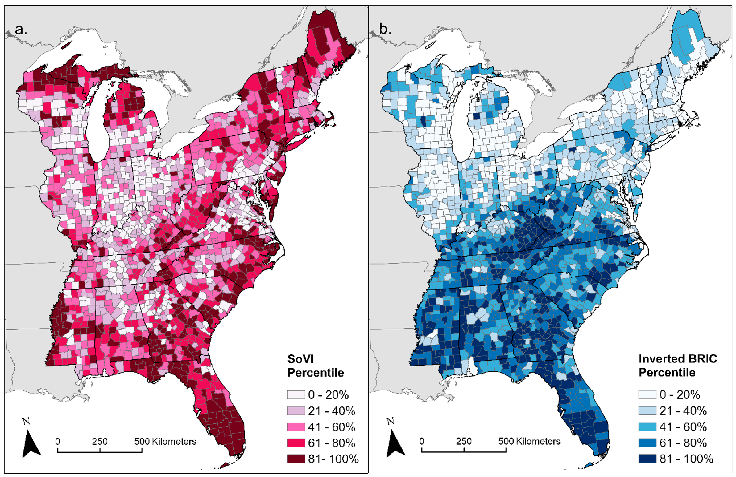
3.1. Patterns of Wildfire Exposure, Social Vulnerability, and Community Resilience

The raster of exposure shows large parts of the study area with no wildfire exposure (Figure 3a), though when consolidated to vector at the county scale, only nineteen counties have no exposed area (Figure 3b). These counties are small, urban counties in Virginia (n = 17), New York (n = 1), and Rhode Island (n = 1). The percent area of a county exposed to at least one wildfire between 2000 and 2020 ranges from 0 to 84.9%, with an average of 14.5% area exposed. Using percentiles at the county scale (Figure 3b), wildfire exposure is concentrated in the southeastern states of Mississippi, Alabama, Georgia, Florida, and South Carolina, with most of these states in the highest percentile category used (80–100%). The areas of lowest exposure include the Northeast, northern New England, parts of Michigan’s Upper Peninsula, and northern Wisconsin.

The lowest exposure counties (excluding those with no exposure) are geographically dispersed in the northern states (

Table 3. Most and least wildfire-exposed counties 2000–2020 ¹.

Least Exposed Counties	Exposure Percentile	Most Exposed Counties	Exposure Percentile
Hamilton, New York	1.2	Baker, Georgia	100
Putnam, New York	1.2	Chattahoochee, Georgia	99.9
Waynesboro, Virginia	1.3	Decatur, Georgia	99.9
Cortland, New York	1.4	Thomas, Georgia	99.8
Keweenaw, Michigan	1.4	Mitchell, Georgia	99.8

¹ Excludes counties with 0 (or no) wildfire exposure.

). The least wildfire-exposed counties include Hamilton County, part of the preserved Adirondack Park in New York, Cortland County in upstate New York, and Keweenaw County in Michigan’s Upper Peninsula, which contains the Isle Royale National Park. The other least exposed counties include suburban Putnam County within metropolitan New York City and Waynesboro, an independent city in Virginia’s Shenandoah Valley.

Florida has the most counties in the top exposure percentile (>80%). Almost all counties in the top exposure quintile are in the Southeast, excluding a few in Virginia and the Appalachian regions of Kentucky and West Virginia. The top five most exposed counties are all located in southwestern Georgia, a state with significant timberland (approximately 9.7 million hectares) and cropland. Chattahoochee (home to Fort Moore) and Thomas Counties have some fires listed in the ancillary datasets. However, most fires in these counties have no cause determined; those with a cause list prescribed burning. The three counties with the highest exposure percentiles in Florida are Wakulla, Liberty, and Jefferson Counties, which are all adjacent and located in the Florida panhandle. All three counties have fires in both ancillary databases, and the leading cause of fires is human (e.g., debris burning) distantly followed by lightning.

In the 26-state study area, SoVI explains 72.9% of the variance among the 28 variables and highlights the six factors of social vulnerability in the study region: (1) less education, (2) age dependency (elderly), (3) family structure (single parent and female-headed households) and race (African American), (4) linguistic isolation and ethnicity (Hispanic), (5) special needs populations (living in nursing homes and group quarters), and (6) Native American populations. SoVI scores range from −5.06 to 23.21 (least to most vulnerable), with an average SoVI score of −0.001. As noted earlier, the scores were converted to percentiles for comparison purposes.

Mapping the percentiles of SoVI shows that high social vulnerability is concentrated in four geographic regions (Figure 4a). The northern group of counties stretching from Michigan’s Upper Peninsula to Upstate New York and north Maine is one region where age (elderly), disability, and lower incomes drive higher social vulnerability scores. The second region is in portions of central Appalachia where social vulnerability is a function of unemployment, poverty, education, disability, and employment in extractive industries. In the South, two regions of social vulnerability are apparent. First, the traditional cotton belt stretches from the coastal plains of North Carolina south and westward to the Mississippi Delta region, where the driving factors of social vulnerability are race and gender, poverty, education, and unemployment. The second distinct region in the South is South Florida, where drivers of social vulnerability are age (elderly), ethnicity, and special needs populations.

There is considerable variability within and between the states in the driving factors producing high social vulnerability (

Table 4. Top ten most socially vulnerable counties in the study region and primary drivers.

Rank	County, State	Percentile	SoVI Score	Most Significant Factors	Population (pop/sq. km) 1
1	Menominee, WI	100.00	23.21	Native American populations	4255 (5)
2	Bronx, NY	99.94	14.01	Ethnicity and linguistic isolation; family structure and race (African American)	1,472,654 (13,483)
3	Swain, NC	99.88	11.17	Native American populations	14,117 (10)
4	Hancock, GA	99.81	11.11	Family structure and race (African American)	8735 (7)
5	Forest, PA	99.75	10.63	Living in group quarters, age (elderly)	6973 (6)
6	Stewart. GA	99.69	10.53	Living in group quarters, poverty	5314 (5)
7	Issaquena, MS	99.63	9.86	Living in group quarters, poverty	1338 (1)
8	Queens, NY	99.56	9.53	Ethnicity and linguistic isolation	2,405,464 (8542)
9	Robeson, NC	99.50	9.04	Native American populations	116,530 (47)
10	New York, NY	99.44	8.96	Ethnicity and linguistic isolation	1,694,251 (28,873)

¹ The 2020 Census population, April 2020. Source: U.S. Census, Quick Facts. Population density rounded to whole number.

). One of the primary drivers of social vulnerability among the top ten most socially vulnerable counties is the presence of Native American populations. These include Menominee, WI, with the Menominee Indian Reservation; Swain, NC, with the Cherokee Indian Reservation; and Robeson, NC, with Tribe, the latter not receiving full federal tribal recognition until 2022 [56]. Three of the most socially vulnerable counties are in New York City (Bronx, Queens, and New York (Manhattan)). In these highly urbanized counties, the driving factors are ethnicity, high proportions of non-English speaking residents, and female-headed households. Three rural southern counties, Hancock and Stewart, GA, and Issaquena, MS, have high social vulnerability levels driven by race (African American), poverty, and aging populations living in group quarters. Lastly, Forest County, PA, is a rural county that contains the Forest State Penitentiary.

BRIC calculations for the 26-state study area range from 1.9 to 3.1, with an average score of 2.6. Mapping the inverse of BRIC using percentiles shows a large regional divide with higher resilience (i.e., lower percentiles) in the Northeast and Midwest and lower community resilience (i.e., higher percentiles) in the South and Appalachia (Figure 4b). There are striking regional patterns in community resilience at the county level, dividing northern from southern states. Within the southern states, there are some distinct sub-state clusters of counties with the least resilience. These include counties in the Appalachian region stretching from southern West Virginia to eastern Kentucky and Tennessee. Other clusters are the coastal plains of southern Georgia and Alabama, the Big Bend area of Florida, and southwestern Florida. The drivers of lower resilience are reduced economic capital and infrastructure/housing capital (

Table 5. Least resilient counties in the study region and capital drivers.

Rank	County, State	Percentile	BRIC Score	Primary Capital Driver	Population Density 1
1	Issaquena County, MS	100.0	1.898	Infrastructure/housing; economic	1
2	Stewart County, GA	99.94	2.012	Infrastructure/housing; community capacity	5
3	Quitman County, GA	99.88	2.024	Infrastructure/housing	6
4	Telfair County, GA	99.81	2.092	Infrastructure/housing	11
5	Hendry County, FL	99.75	2.101	Infrastructure/housing	13
6	Glades County, FL	99.69	2.121	Infrastructure/housing	6
7	DeSoto County, FL	99.63	2.141	Infrastructure/housing	20
8	Mingo County, WV	99.56	2.147	Infrastructure/housing	22
9	McDowell County, WV	99.50	2.148	Infrastructure/housing	14
10	Echols County, GA	99.44	2.152	Infrastructure/housing	3

¹ The 2020 population per square kilometer. Source: U.S. Census, Quick Facts.

).

All these counties are rural and isolated counties with small populations. Issaquena County, MS (population 1338), has the lowest per capita income of any county in the nation, which is a main driver of the lack of economic capital, and when coupled with very low infrastructure/housing capital, makes it the least resilient county in our study area. Stewart, GA (population 5314), also has low infrastructure/housing capital and very low community capital (e.g., lacking in political engagement, social capital, and place attachment) when compared to the other nine counties. The infrastructure/housing resilience drivers are related to lower access to medical care, high-speed internet, sturdier housing types (e.g., not mobile homes), and housing stock and availability. The remaining Georgia counties are all rural and isolated in southern Georgia. Quitman County is very small in area (391.71 square kilometers, 6% of which is water) with a population of 2235. In Florida, the least resilient counties (Hendry and Glades) are on the western border of Lake Okeechobee, while DeSoto County, inland of Port Charlotte on Florida’s west coast, is also rural (population density of 20 people per square kilometer). Mingo and McDowell counties in West Virginia border Kentucky and Virginia, respectively.

3.2. Delineating Disadvantaged Communities

The relative levels of social vulnerability and inherent community resilience define disadvantaged communities. Overall, disadvantaged counties are rural, the exceptions being inland counties in South Florida and counties in the New York metropolitan area. Spatially, concentrations of the most disadvantaged counties appear in eastern Kentucky, western North Carolina, the inner coastal plains stretching from North Carolina to southern Georgia, and the lower Mississippi River Valley region (Figure 5). The least disadvantaged places are rural to suburban counties with average incomes, little racial diversity, and households with married couples with children, generally located in the Midwestern states in our study area (

Table 6. Most and least disadvantaged counties.

Most Disadvantaged	Percentile	Least Disadvantaged	Percentile
Stewart, GA	99.81	Calumet, WI	0.31
Issaquena, MS	99.81	Putnam, OH	0.75
Hancock, GA	99.47	Poquoson, VA	0.81
Hendry, FL	99.31	Ozaukee, WI	1.21
Quitman, GA	99.31	Union, OH	1.40
DeSoto, FL	99.16	Washington, WI	1.68
Telfair, GA	99.13	Mercer, OH	1.93
Glades, FL	98.82	Ottawa, MI	2.09
Bronx, NY	98.53	Auglaize, OH	2.09
Macon, GA	98.31	Waukesha, WI	2.12

). The five most and least disadvantaged counties are highlighted in Figure 5 in red and blue, respectively, graphically illustrating the regional divide of disadvantage as measured through SoVI and BRIC.

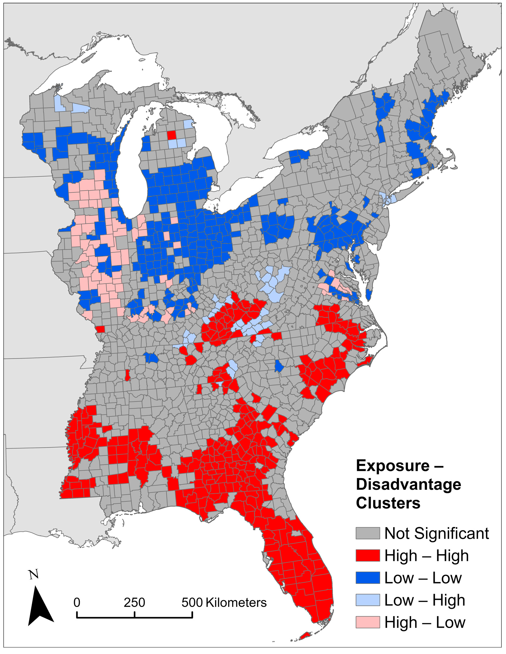
3.3. Social Burdens of Uneven Exposures

The relationship between wildfire exposure and disadvantaged communities highlights uneven social burdens within the study area. For example, lower exposure percentiles are associated with lower disadvantage (

Table 7. Relationship of exposure percentile to disadvantaged counties.

	Wildfire Exposure Ranking
	Bottom 20%	21–40%	41–60%	61–80%	Top 20%
Number of Counties	337	321	321	321	305
Mean Disadvantaged ranking	43.27	37.71	40.86	57.13	72.47
Mean Social Vulnerability ranking	54.75	38.62	38.80	50.71	67.76
Mean Resilience ranking	31.80	36.80	42.93	63.55	77.19

). The mean ranking for disadvantaged counties in the top 20% of exposure is 72.47, while in the bottom 20% of exposure, the mean percentile ranking is 43.27 (less disadvantage). The lowest exposure counties contain, on average, a larger number of socially vulnerable counties that are primarily urban. The counties with exposure percentiles between 21 and 40% have the lowest mean disadvantaged ranking and lowest mean SoVI percentile ranking. These are generally smaller metropolitan counties. However, the areas with the lowest exposure (bottom 20%) also have the lowest resilience percentile ranking, meaning they have more resilience.

According to a one-way ANOVA, the differences between social vulnerability and resilience values in each exposure quintile are statistically different (SoVI F = 50.21, p < 0.001; BRIC F = 193.5, p < 0.001). Further, Spearman’s rank correlation between exposure percentile and SoVI, BRIC, and disadvantaged percentiles is significant (p < 0.01) but strongest with BRIC (r_s = 0.573). Social vulnerability is only weakly associated (r_s = 0.171) with wildfire exposure.

Exposure and disadvantaged percentiles are clustered (Global Moran’s I = 0.855 and =0.580, respectively, with p < 0.01). A bi-variate local Moran’s I in GeoDa shows the spatial relationship of clusters and outliers of high and low values in both exposure and disadvantaged percentiles (Figure 6). Here, the relationship between exposure and disadvantaged communities is depicted spatially. Lower percentiles of exposure and disadvantage are generally in the northern half of the study area, but there are outliers of high exposure with low disadvantage, primarily focused in Illinois, southern Michigan, and parts of eastern Virginia. The areas of highest disadvantage and highest exposure follow spatial clusters of social vulnerability (i.e., the Cotton Belt, Appalachia, and southern Florida). Some outliers of low wildfire exposure but high disadvantage are located in parts of Appalachia in Kentucky, Virginia, and West Virginia.

Three isolated high exposure and high disadvantaged counties stand out: Crawford County, MI; Union County, IL; and Decatur County, TN. These counties are rural and are declining in population, with between 14 and 20% of their populations living in poverty. Across the three counties, state and federal entities own much of their land. For example, Crawford County has nearly 75% of its land in public ownership, which includes Camp Grayling, a military base used for training the National Guard. Some isolated areas of low exposure and low disadvantage are Mecklenburg County, NC, and Davidson and Cheatham Counties in Tennessee. Mecklenburg County is home to Charlotte, and Davidson County houses Nashville, with Cheatham County directly neighboring. These three counties have younger, wealthier, and growing populations with less wildfire exposure due to the relatively developed nature of the county.

This analysis illustrates that wildfire exposure, social vulnerability, and community resilience vary spatially as anticipated. However, there are strong regional patterns in the variability in exposure and community resilience, the former showing higher concentrations in the southern states and Florida, the latter showing greater resilience in counties in northern states. When creating disadvantaged counties using social vulnerability and community resilience, parts of the South regularly show more disadvantaged counties, suggesting they are not only socially vulnerable but also lacking in community resilience. When comparing disadvantaged counties to wildfire exposure, the most disadvantaged counties are also more exposed. This is primarily driven by the lack of community resilience more than social vulnerability. Lastly, when comparing disadvantaged places to wildfire exposure spatially, the regional divide between the Southeast and Northeast is clearly visible, including southern Appalachia with its high exposure and high level of disadvantage. There are some patches of higher wildfire exposure with low disadvantage in and around Illinois and some interesting, isolated cases of high exposure and high disadvantage in rural counties in Illinois, Michigan, and Tennessee.

4. Discussion

The pattern of exposure identified through the MODIS, VIIRS, and ancillary datasets is similar to patterns of wildfire exposure previously identified in the South using a similar methodology [49], but we found a more extensive distribution of wildfire. In studies of the entire United States, for example, regions of high exposure in Appalachia, Florida, and the Gulf Coast are included; however, the high exposure in Georgia and the moderate exposure in western Tennessee and Illinois are missing [57]. This is likely due to the inclusion parameters and reporting methods used in other datasets that only include fires over a certain size and source data from in-person reporting. The fires included in our exposure surface have a high confidence and include smaller fires due to the higher resolution of the satellite data used.

This study has found several distinct spatial patterns of wildfire exposure and social disadvantage in the Eastern United States. Exposure in the Eastern U.S. can be characterized as high-probability, low-impact events, with most exposure focused in the South and extending to Illinois. Most fires in the study area can be attributed to human causes such as prescribed burning, conducted for a variety of purposes (e.g., habitat maintenance, agriculture, wildfire risk mitigation) [41,58], or debris burning [59]. In addition, annual crop and property loss in the East is comparatively low, supporting the conclusion that the fires in this region, although they happen often, currently have low impacts.

This result has two implications: the current burden of wildfire in the Eastern U.S. is likely more related to the distal impacts of wildfire, such as smoke, and the future projections of where and when prescribed burns can take place are integral in understanding how wildfire exposure will change. Due to climate change, increasing WUI, and institutional constraints, prescribed burn windows will likely be reduced [60], decreasing the regular distal impacts of fire in the region but increasing the risk of larger, uncontrolled fires that prescribed burning currently mitigates.

However, exposure is only part of the story of wildfire in the eastern states, where the social burdens are potentially more significant. We have found that social vulnerability, community resilience, and the drivers of both differ by region. Much of the extant research highlighting the social impacts of wildfires has generally considered the demographic or socioeconomic characteristics of potentially exposed individuals or communities. Few have also considered the capacity of the communities to prepare for, respond to, recover from, or adapt to this particular hazard. Combining two measures of how well a community (i.e., county) can prepare and adapt and how susceptible it is to hazards is important and an advancement in providing a broader view of wildfire risk.

Previous work has shown that social vulnerability and community resilience are related but not opposing concepts [61,62]. It is important to consider both, and in this case, we can do so in a simple and replicable way. Defining disadvantaged places with both social vulnerability and community resilience metrics provides a more robust, empirical based definition, and spatial representation of disadvantage. The utility of these indices is that their summary number (e.g., SoVI score, BRIC score), which can be used for analysis, can also be broken down into component parts regarding policy decisions, outreach, education, and stakeholder engagement. Further, determining the drivers of social vulnerability and resilience for different regions explores how these concepts are place-based, requiring different interventions depending on location and social dimensions [14].

The analysis of this study focuses solely on the occurrence of fire events to model exposure to wildfire, though the fires themselves do not act alone in affecting populations in close proximity. The geographic extent of smoke exposure moves well beyond the fire event alone. Smoke exposure from wildfires significantly impacts lower socio-economic groups especially, and future quantitative geographic studies could provide more robust analysis on what type of communities are impacted by well-traveled smoke in the Eastern U.S. [2,63,64]. This study has also refrained from making causative statements regarding fire exposure and social vulnerability and resilience, though the approach has suggested a strong relationship where communities with more vulnerability and lower resilience are disproportionately affected.

There are several caveats and limitations to this research due to its geographic focus and methodology. The goal of this study was to conduct an initial examination of the spatial patterns of wildfire exposure in disadvantaged communities in the Eastern U.S. There is a trade-off between capturing as many fires over the study period as possible and losing the attributes of each fire included in the final dataset. We could only identify exposed and non-exposed areas in the final raster exposure surface according to areas that had burned sometime between 2000 and 2020. This does not mean that areas that did not burn in this time period could not burn in the future and further research should attempt to reintroduce fire recurrence, economic impact, and measures of WUI to expand exposure from the binary presented here. In addition, MODIS and VIIRS data have their own limitations, including the effect of cloud cover on data collection. Future work can include even more ancillary data (e.g., Landsat, geotagged social media posts) to further validate the exposure surface created.

In addition, all measures of exposure, SoVI, and BRIC are aggregated or calculated at the county level. Future work should consider sub-county variations in these three. The wildfire raster surfaces were aggregated at the county level so they could be compared to county-level calculations of SoVI and BRIC. Counties are still large areas in which wildfires can occur away from populations or in the WUI where there could be more exposure, but this spatial variation is lost in the analysis at our scale.

Calculating SoVI to a sub-county scale is possible, but using census tracts, which is a common approach to downscaling social indices, has no real meaning vis-à-vis a community since they are just administrative units for social, demographic, and economic data. Future research should explore thinking about community in this context as incorporated vs. non-incorporated places, whereby data could be distributed via dasymetric mapping based on population and land cover that could then be merged with pixel or point wildfire exposure data.

Unfortunately, our input measure of community resilience, BRIC, is challenging to compute at the sub-county scale since it relies on datasets other than the census. There are ongoing tests of BRIC constructions that compare county data and constructions to their census tract counterparts that show a relatively high correlation between the two [65], so a simple extraction of county BRIC would provide a generalized indicator at the census tract level, but there would be no variability among tracts within any given county. Deconstructing the vulnerability and resilience data from vector to raster would be another approach for comparing wildfire exposure, social vulnerability, and community resilience measurements. This might offer the most fruitful approach going forward.

5. Conclusions

Within the Eastern U.S., there is a distinct pattern of wildfire exposure. The Southeast has the highest exposure, and fires are likely human-caused and prescribed burning. However, including dimensions of the social burdens of exposure is essential. Creating a measure of disadvantaged counties using social vulnerability and community resilience illustrates where those wildfire exposures could have the greatest adverse impact—areas with highly vulnerable populations and relatively little community capacity to adequately respond to potential events. Thus, in thinking about wildfire risk, we argue risk is not only exposure but equally important is the inclusion of disadvantaged places (incorporating social vulnerability and community resilience) in understanding the differential impact of wildfire on people and places where they live.

The risk of wildfire will change, especially in the Southeast, as prescribed burning windows change due to increased development in WUI, climate change, and regulations. More detailed analysis at sub-county scales may prove fruitful in overcoming some of the limitations of this research in terms of input data. Also, it would be significant to extend the analysis to western states to see how well the initial computation of a generalized wildfire exposure model performs using high-resolution datasets, social vulnerability, and community resilience indicators to define the differential risk of wildfires in disadvantaged communities.

References

1. NOAA National Centers for Environmental Information (NCEI) U.S. Billion-Dollar Weather and Climate Disasters (2024). Available online: https://www.ncei.noaa.gov/access/billions/ (accessed on 29 March 2024).
2. Burke, M.; Driscoll, A.; Heft-Neal, S.; Xue, J.; Burney, J.; Wara, M. The Changing Risk and Burden of Wildfire in the United States. Proc. Natl. Acad. Sci. USA 2021, 118, e2011048118. [Google Scholar] [CrossRef] [PubMed]
3. Radeloff, V.C.; Helmers, D.P.; Kramer, H.A.; Mockrin, M.H.; Alexandre, P.M.; Bar-Massada, A.; Butsic, V.; Hawbaker, T.J.; Martinuzzi, S.; Syphard, A.D.; et al. Rapid Growth of the US Wildland-Urban Interface Raises Wildfire Risk. Proc. Natl. Acad. Sci. USA 2018, 115, 3314–3319. [Google Scholar] [CrossRef] [PubMed]
4. Carlson, A.R.; Sebasky, M.E.; Peters, M.P.; Radeloff, V.C. The Importance of Small Fires for Wildfire Hazard in Urbanised Landscapes of the Northeastern US. Int. J. Wildland Fire 2021, 30, 307–321. [Google Scholar] [CrossRef]
5. Prestemon, J.P.; Shankar, U.; Xiu, A.; Talgo, K.; Yang, D.; Dixon, E.; McKenzie, D.; Abt, K.L. Projecting Wildfire Area Burned in the South-Eastern United States, 2011–2060. Int. J. Wildland Fire 2016, 25, 715–729. [Google Scholar] [CrossRef]
6. Radeloff, V.C.; Mockrin, M.H.; Helmers, D.; Carlson, A.; Hawbaker, T.J.; Martinuzzi, S.; Schug, F.; Alexandre, P.M.; Kramer, H.A.; Pidgeon, A.M. Rising Wildfire Risk to Houses in the United States, Especially in Grasslands and Shrublands. Science 2023, 382, 702–707. [Google Scholar] [CrossRef]
7. Boomhower, J. Adapting to Growing Wildfire Property Risk. Science 2023, 382, 638–641. [Google Scholar] [CrossRef]
8. Gao, P.; Terando, A.J.; Kupfer, J.A.; Morgan Varner, J.; Stambaugh, M.C.; Lei, T.L.; Kevin Hiers, J. Robust Projections of Future Fire Probability for the Conterminous United States. Sci. Total Environ. 2021, 789, 147872. [Google Scholar] [CrossRef] [PubMed]
9. Lambrou, N.; Kolden, C.; Loukaitou-Sideris, A.; Anjum, E.; Acey, C. Social Drivers of Vulnerability to Wildfire Disasters: A Review of the Literature. Landsc. Urban Plan. 2023, 237, 104797. [Google Scholar] [CrossRef]
10. USDA Forest Service. Understand Risk. 8 March 2023. Available online: https://wildfirerisk.org/understand-risk/#:~:text=About%20Exposure&text=Any%20community%20that%20is%20located,forest%20is%20exposed%20to%20wildfire (accessed on 29 March 2024).
11. Tierney, K.J. Disasters: A Sociological Approach; Polity Press: Medford, MA, USA, 2020. [Google Scholar]
12. Cutter, S.L.; Boruff, B.J.; Shirley, W.L. Social Vulnerability to Environmental Hazards. Soc. Sci. Q. 2003, 84, 242–261. [Google Scholar] [CrossRef]
13. National Research Council. Disaster Resilience: A National Imperative; National Academies Press: Washington, DC, USA, 2012. [Google Scholar]
14. Davies, I.P.; Haugo, R.D.; Robertson, J.C.; Levin, P.S. The Unequal Vulnerability of Communities of Color to Wildfire. PLoS ONE 2018, 13, e0205825. [Google Scholar] [CrossRef]
15. Wigtil, G.; Hammer, R.B.; Kline, J.D.; Mockrin, M.H.; Stewart, S.I.; Roper, D.; Radeloff, V.C. Places Where Wildfire Potential and Social Vulnerability Coincide in the Coterminous United States. Int. J. Wildland Fire 2016, 25, 896–908. [Google Scholar] [CrossRef]
16. LSLR Collaborative. Defining Disadvantaged Communities. Available online: https://www.lslr-collaborative.org/defining-disadvantaged-communities.html (accessed on 8 January 2024).
17. Lee, C. Evaluating Environmental Protection Agency’s Definition of Environmental Justice. Environ. Justice 2021, 14, 332–337. [Google Scholar] [CrossRef]
18. White House. Executive Order (#13985) On Advancing Racial Equity and Support for Underserved Communities Through the Federal Government. Available online: https://www.whitehouse.gov/briefing-room/presidential-actions/2021/01/20/executive-order-advancing-racial-equity-and-support-for-underserved-communities-through-the-federal-government/ (accessed on 8 January 2024).
19. White House. Justice40 Initiative: A Whole-of-Government Initiative. Available online: https://www.whitehouse.gov/environmentaljustice/justice40/ (accessed on 14 December 2023).
20. White House. Climate and Economic Justice Screening Tool: Frequently Asked Questions. Available online: https://screeningtool.geoplatform.gov/en/frequently-asked-questions (accessed on 14 December 2023).
21. Peacock, W.G.; Van Zandt, S.; Zhang, Y.; Highfield, W.E. Inequities in Long-Term Housing Recovery After Disasters. J. Am. Plann. Assoc. 2014, 80, 356–371. [Google Scholar] [CrossRef]
22. Emrich, C.T.; Tate, E.; Larson, S.E.; Zhou, Y. Measuring Social Equity in Flood Recovery Funding. Environ. Hazards. 2020, 19, 228–250. [Google Scholar] [CrossRef]
23. Coughlan, M.R.; Ellison, A.; Cavanaugh, A.H. Social Vulnerability and Wildfire in the Wildland-Urban Interface: A Literature Synthesis; Ecosystem Workforce Program, Institute for a Sustainable Environment, University of Oregon: Eugene, OR, USA, 2019. [Google Scholar]
24. Akter, S.; Grafton, R.Q. Do Fires Discriminate? Socio-Economic Disadvantage, Wildfire Hazard Exposure and the Australian 2019–20 ‘Black Summer’ Fires. Clim. Change 2021, 165, 53. [Google Scholar] [CrossRef]
25. Andersen, L.M.; Sugg, M.M. Geographic Multi-Criteria Evaluation and Validation: A Case Study of Wildfire Vulnerability in Western North Carolina, USA Following the 2016 Wildfires. Int. J. Disaster. Risk Reduct. 2019, 39, 101123. [Google Scholar] [CrossRef]
26. Bergonse, R.; Oliveira, S.; Santos, P.; Zêzere, J.L. Wildfire Risk Levels at the Local Scale: Assessing the Relative Influence of Hazard, Exposure, and Social Vulnerability. Fire 2022, 5, 166. [Google Scholar] [CrossRef]
27. Chase, J.; Hansen, P. Displacement after the Camp Fire: Where Are the Most Vulnerable? Soc. Nat. Resourc. 2021, 34, 1566–1583. [Google Scholar] [CrossRef]
28. Schumann, R.L.; Emrich, C.T.; Butsic, V.; Mockrin, M.H.; Zhou, Y.; Johnson Gaither, C.; Price, O.; Syphard, A.D.; Whittaker, J.; Aksha, S.K. The Geography of Social Vulnerability and Wildfire Occurrence (1984–2018) in the Conterminous USA. Nat. Hazards. 2024, 120, 4297–4327. [Google Scholar] [CrossRef]
29. Auer, M.R.; Hexamer, B.E. Income and Insurability as Factors in Wildfire Risk. Forests 2022, 13, 1130. [Google Scholar] [CrossRef]
30. Palaiologou, P.; Ager, A.A.; Nielsen-Pincus, M.; Evers, C.R.; Day, M.A. Social Vulnerability to Large Wildfires in the Western USA. Landsc. Urban Plan. 2019, 189, 99–116. [Google Scholar] [CrossRef]
31. Wibbenmeyer, M.; Robertson, M. The Distributional Incidence of Wildfire Hazard in the Western United States. Environ. Res. Lett. 2022, 17, 064031. [Google Scholar] [CrossRef]
32. Masri, S.; Scaduto, E.; Jin, Y.; Wu, J. Disproportionate Impacts of Wildfires among Elderly and Low-Income Communities in California from 2000–2020. Int. J. Environ. Res. Public Health 2021, 18, 3921. [Google Scholar] [CrossRef] [PubMed]
33. Kulig, J.; Botey, A.P. Facing a Wildfire: What Did We Learn about Individual and Community Resilience? Nat. Hazards. 2016, 82, 1919–1929. [Google Scholar] [CrossRef]
34. Thomas, A.S.; Escobedo, F.J.; Sloggy, M.R.; Sánchez, J.J. A Burning Issue: Reviewing the Socio-Demographic and Environmental Justice Aspects of the Wildfire Literature. PLoS ONE 2022, 17, e0271019. [Google Scholar] [CrossRef]
35. National Association of Counties (NACO). Building Wildfire Resilience: A Land Use Toolbox for County Leaders. Available online: https://www.naco.org/resources/building-wildfire-resilience (accessed on 14 December 2023).
36. U.S. Census Bureau. State Population Data Summary File. 2020. Available online: https://www.census.gov/library/visualizations/interactive/2020-population-and-housing-state-data.html (accessed on 28 March 2024).
37. Monitoring Trends in Burn Severity (MTBS). National Fire Occurence Dataset; USGS: Reston, VA, USA, 2024. [Google Scholar]
38. Center for Emergency Management and Homeland Security (CEMHS). In Spatial Hazard Events and Losses Database for the United States (SHELDUS); Center for Emergency Management and Homeland Security (CEMHS): Phoenix, AZ, USA, 2024.
39. Salguero, J.; Li, J.; Farahmand, A.; Reager, J.T. Wildfire Trend Analysis over the Contiguous United States Using Remote Sensing Observations. Remote Sens. 2020, 12, 2565. [Google Scholar] [CrossRef]
40. Carter, L.M.; Terando, A.; Dow, K.; Hiers, K.; Kunkel, K.E.; Lascurain, A.; Marcy, D.C.; Osland, M.J.; Schramm, P.J. Southeast. Impacts, Risks, and Adaptation in the United States. In The Fourth National Climate Assessment; Reidmiller, D.R., Avery, C.W., Easterling, D.R., Kunkel, K.E., Lewis, K.L.M., Maycock, T.K., Stewart, B.C., Eds.; U.S. Global Change Research Program: Washington, DC, USA, 2018; Volume II, pp. 743–808. [Google Scholar]
41. Cummins, K.; Noble, J.; Varner, J.M.; Robertson, K.M.; Hiers, J.K.; Nowell, H.K.; Simonson, E. The Southeastern U.S. Prescribed Fire Permit Database: Hot Spots and Hot Moments in Prescribed Fire across the Southeastern USA. Fire 2023, 6, 372. [Google Scholar] [CrossRef]
42. Cattau, M.E.; Mahood, A.L.; Balch, J.K.; Wessman, C.A. Modern Pyromes: Biogeographical Patterns of Fire Characteristics across the Contiguous United States. Fire 2022, 5, 95. [Google Scholar] [CrossRef]
43. Giglio, L.; Descloitres, J.; Justice, C.O.; Kaufman, Y.J. An Enhanced Contextual Fire Detection Algorithm for MODIS. Remote Sens. Environ. 2003, 87, 273–282. [Google Scholar] [CrossRef]
44. Schroeder, W.; Oliva, P.; Giglio, L.; Csiszar, I.A. The New VIIRS 375m Active Fire Detection Data Product: Algorithm Description and Initial Assessment. Remote Sens. Environ. 2014, 143, 85–96. [Google Scholar] [CrossRef]
45. Giglio, L.; Schroeder, W.; Hall, J.V. MODIS Collection 6 Active Fire Product User’s Guide, Revision C; NASA: Washington, DC, USA, 2020.
46. Welty, J.; Jeffries, M. Combined Wildland Fire Datasets for the United States and Certain Territories, 1800s-Present [Data Set]; U.S. Geological Survey: Reston, VA, USA, 2021. [Google Scholar] [CrossRef]
47. Wildland Fire Interagency Geospatial Services (WFIGS). Wildland Fire Locations Full History; National Interagency Fire Center: Boise, ID, USA, 2021.
48. Dewitz, J. National Land Cover Database (NLCD) 2019 Products (ver 2.0); U.S. Geological Survey: Reston, VA, USA, 2021. [Google Scholar]
49. Federal Aviation Administration (FAA), Digital Obstacle File [Data set]. 2023. Available online: https://www.faa.gov/air_traffic/flight_info/aeronav/digital_products/dof/ (accessed on 4 April 2024).
50. Korontzi, S.; McCarty, J.; Justice, C. Monitoring Agricultural Burning in the Mississippi River Valley Region from the Moderate Resolution Imaging Spectroradiometer (MODIS). J. Air Waste Manag. Assoc. 2008, 58, 1235–1239. [Google Scholar] [CrossRef]
51. McCarty, J.L.; Justice, C.O.; Korontzi, S. Agricultural Burning in the Southeastern United States Detected by MODIS. Remote Sens. Environ. 2007, 108, 151–162. [Google Scholar] [CrossRef]
52. Hazards Vulnerability and Resilience Institute. SoVI®. Available online: https://sc.edu/study/colleges_schools/artsandsciences/centers_and_institutes/hvri/data_and_resources/sovi/index.php (accessed on 7 February 2024).
53. Zuzak, C.; Goodenough, E.; Stanton, C.; Mowrer, M.; Sheehan, A.; Roberts, B.; McGuire, P.; Rozelle, J. National Risk Index Technical Documentation; Federal Emergency Management Agency: Washington, DC, USA, 2023. [Google Scholar]
54. Hazards Vulnerability and Resilience Institute. BRIC. Available online: https://sc.edu/study/colleges_schools/artsandsciences/centers_and_institutes/hvri/data_and_resources/bric/index.php (accessed on 7 February 2024).
55. Cutter, S.L.; Ash, K.D.; Emrich, C.T. The Geographies of Community Disaster Resilience. Glob. Environ. Change 2014, 29, 65–77. [Google Scholar] [CrossRef]
56. Rep. Butterfield, G.K. [D-N.-1 H.R.2758—117th Congress (2021–2022): Lumbee Recognition Act. Available online: https://www.congress.gov/bill/117th-congress/house-bill/2758 (accessed on 7 February 2024).
57. Strader, S.M. Spatiotemporal Changes in Conterminous US Wildfire Exposure from 1940 to 2010. Nat. Hazards. 2018, 92, 543–565. [Google Scholar] [CrossRef]
58. Terando, A.J.; Kupfer, J.A.; Gao, P.; Teske, C.; Hiers, K.J. Prescribed Fire Permit Records for Georgia and Florida [Data set]; U.S. Geological Survey. 2019. Available online: https://catalog.data.gov/dataset/prescribed-fire-permit-records-for-georgia-and-florida (accessed on 4 April 2024).
59. Nagy, R.C.; Fusco, E.; Bradley, B.; Abatzoglou, J.T.; Balch, J. Human-Related Ignitions Increase the Number of Large Wildfires across U.S. Ecoregions. Fire 2018, 1, 4. [Google Scholar] [CrossRef]
60. Kupfer, J.A.; Lackstrom, K.; Grego, J.M.; Dow, K.; Terando, A.J.; Hiers, J.K. Prescribed Fire in Longleaf Pine Ecosystems: Fire Managers’ Perspectives on Priorities, Constraints, and Future Prospects. Fire Ecol. 2022, 18, 27. [Google Scholar] [CrossRef]
61. Derakhshan, S.; Emrich, C.T.; Cutter, S.L. Degree and Direction of Overlap between Social Vulnerability and Community Resilience Measurements. PLoS ONE 2022, 17, e0275975. [Google Scholar] [CrossRef] [PubMed]
62. Lanlan, J.; Sarker, M.N.I.; Ali, I.; Firdaus, R.B.R.; Hossin, M.A. Vulnerability and Resilience in the Context of Natural Hazards: A Critical Conceptual Analysis. Environ. Dev. Sustain. 2023. [Google Scholar] [CrossRef]
63. Casey, J.A.; Kioumourtzoglou, M.-A.; Padula, A.; González, D.J.; Elser, H.; Aguilera, R.; Northrop, A.J.; Tartof, S.Y.; Mayeda, E.R.; Braun, D.; et al. Measuring long-term exposure to wildfire PM 2.5 in California: Time-varying inequities in environmental burden. Proc. Natl. Acad. Sci. USA 2024, 121, e2306729121. [Google Scholar] [CrossRef]
64. Vargo, J.; Lappe, B.; Mirabelli, M.C.; Conlon, K.C. Social vulnerability in US communities affected by wildfire smoke, 2011 to 2021. Am. J. Public Health 2023, 113, 759–767. [Google Scholar] [CrossRef]
65. Derakhshan, S.; Blackwood, L.; Habets, M.; Effgen, J.F.; Cutter, S.L. Prisoners of Scale: Downscaling Community Resilience Measurements for Enhanced Use. Sustainability 2022, 14, 6927. [Google Scholar] [CrossRef]
Figure 1. State comparisons of wildfire frequency (average annual events) and property/crop losses (average annual loss in USD 2022) for 1984–2022.
Fire 07 00124 g001
Figure 2. Wildfire exposure raster and subsequent vector layer creation methodology.
Fire 07 00124 g002
Figure 3. Wildfire exposure based on (a) raster surfaces and (b) percentiles per county based on land area affected.
Fire 07 00124 g003
Figure 4. Quintiles represent the percentiles of county (a) social vulnerability (SoVI), and (b) resilience (BRIC). The bottom quintile (81–100%) represents the most vulnerable and the least resilient counties.
Fire 07 00124 g004
Figure 5. Disadvantaged counties measured by social vulnerability and community resilience. The disadvantaged county in Virginia is geographically small and less visible on the map at this scale.
Fire 07 00124 g005
Figure 6. Bivariate Moran’s I map comparing clusters of exposure percentiles to disadvantaged percentiles.
Fire 07 00124 g006