Abstract
The Manila Clam is an important economic shellfish in China’s seafood industry. In order to improve the design of juvenile Manila Clam seeding equipment, a juvenile clam discrete element method (DEM) particle shape was established, which is based on 3D scanning and EDEM software. The DEM contact parameters of clam-stainless steel, and clam-acrylic were calibrated by combining direct measurements and test simulations (slope sliding and dropping). Then, clam DEM simulation and realistic seeding tests were carried out on a seeding wheel at different rotational speeds. The accuracy of the calibrated clam DEM model was evaluated in a clam seeding verification test by comparing the average error of the variation coefficient between the realistic and simulated seeding tests. The results showed that: (a) the static friction coefficients of clam-acrylic and clam-stainless steel were 0.31 and 0.23, respectively; (b) the restitution coefficients of clam-clam, clam-acrylic, and clam-stainless steel were 0.32, 0.48, and 0.32, respectively. Furthermore, the results of the static repose angle from response surface tests showed that when the contact wall was acrylic, the coefficient rolling friction and static friction of clam-clam were 0.17 and 1.12, respectively, and the coefficient rolling friction of clam-acrylic was 0.20. When the contact wall was formed of stainless steel, the coefficient rolling friction and static friction of clam-clam were 0.33 and 1.25, respectively, and the coefficient rolling friction of clam-stainless steel was 0.20. The results of the verification test showed that the average error between the realistic and simulated value was <5.00%. Following up from these results, the clam DEM model was applied in a clam seeding simulation.
1. Introduction
The Manila Clam (Ruditapes philippinarum) is one of the most important farmed shellfish in China and has high economic benefit. China’s Manila Clam production exceeded 4 × 10⁶ t in 2019 [1]. The seeding quality of juvenile Manila Clams (clam) is an important factor affecting production. Currently, artificial seeding is the foremost clam seeding method and has the problems of high labor intensity, uneven seeding, and considerable product damage [2]. The clams’ mechanized seeding can reduce farming costs and increase economic returns. However, there is no mechanized clam seeding equipment on the market at the moment. Therefore, the development of mechanized seeding equipment is imperative.
If designing clam seeding equipment by traditional empirical design methods, there are disadvantages such as time consumption and high testing cost, and it is difficult to accurately analyze the complex dynamic behavior of clam during the mechanized seeding process. The discrete element method (DEM) can accurately simulate the mechanized seeding of clams and better reflect the state of particles in complex motion, with the advantage of improving design efficiency and cost savings, and DEM has been widely used in the research and design of agricultural equipment [3,4,5,6,7,8]. However, when DEM is used to simulate the seeding process, the accurate DEM particle model (clam DEM shape and simulation contact parameters) is the key factor that can improve the accuracy of the simulation results and is thereby conducive to the structural design of the clam seeding equipment and the actual seeding effect. Due to the morphological and physical trait differences between a clam and the DEM particle model, there will inevitably be some errors between the realistic contact parameters and the simulated contact parameters. Hence, the simulated contact parameters need calibrating [9,10,11].
Several studies on the establishment of an agricultural granular material DEM model and the acquisition of simulation contact parameters have been undertaken. There are two methods to obtain the simulation contact parameters, namely a direct measuring approach and a DEM simulation calibration approach [12]. The contact parameters of some granular materials have been measured directly, e.g., flax seeds [13], corn, and olives [14]. However, the accuracy of the granular material DEM model is low due to the shape differences between reality and simulation, and the subsequent large measuring error [12,15]. The DEM simulation calibration approach, a laboratory-scale experiment, is performed with a granular material, which is then simulated using DEM. The DEM input simulation contact parameters are then repetitively changed until the results are similar to the actual experiment’s outputs [16]. The DEM simulation calibration approach has the advantage of a reduced error and greater accuracy, and it has been widely used in agricultural engineering. Therefore, several studies have calibrated the simulated contact parameters of agricultural granular materials through DEM simulation calibration. The calibration objects include corn [17,18,19,20], dried cherry fruit [21], rice [3,22,23], wheat [11], soybean [24,25], mini-potatoes [9,26], rape stalks [27], peanuts [28], and yams [29]. Although DEM simulation calibration has been widely used in the calibration field, there are still some deficiencies requiring improvements, such as few studies on the simulation calibration of the contact parameters of heterogeneous and live materials, e.g., clam. Not all parameters can be obtained by simulation calibration approach, etc. Therefore, the combination of experimental design method and simulation method was used for predicting the unavailable parameters in this study, so as to achieve the purpose of consistency between simulation effect and actual effect.
To provide more accurate reference to the design and optimization of the clam seeding equipment, the living clams were taken as research objects. A clam DEM particle shape was established, as well as calibration of the simulation contact parameters between clam and various materials. The accuracy of the clam DEM model was verified with a clam seeding test.
2. Materials and Methods
2.1. Materials
In this paper, the calibration object was a 15–20 mm long clam used for seeding in the shellfish farm area of Dandong City, Liaoning Province, China. According to the seeding equipment design requirements, 5 mm thick acrylic and stainless steel plates were selected as the contact wall materials. The initial set of material parameters for acrylic (AC), stainless steel (SS), and clam are shown in Table 1.

Table 1.
The initial set of material parameters for AC, SS, and Clam.
2.2. Clam DEM Model
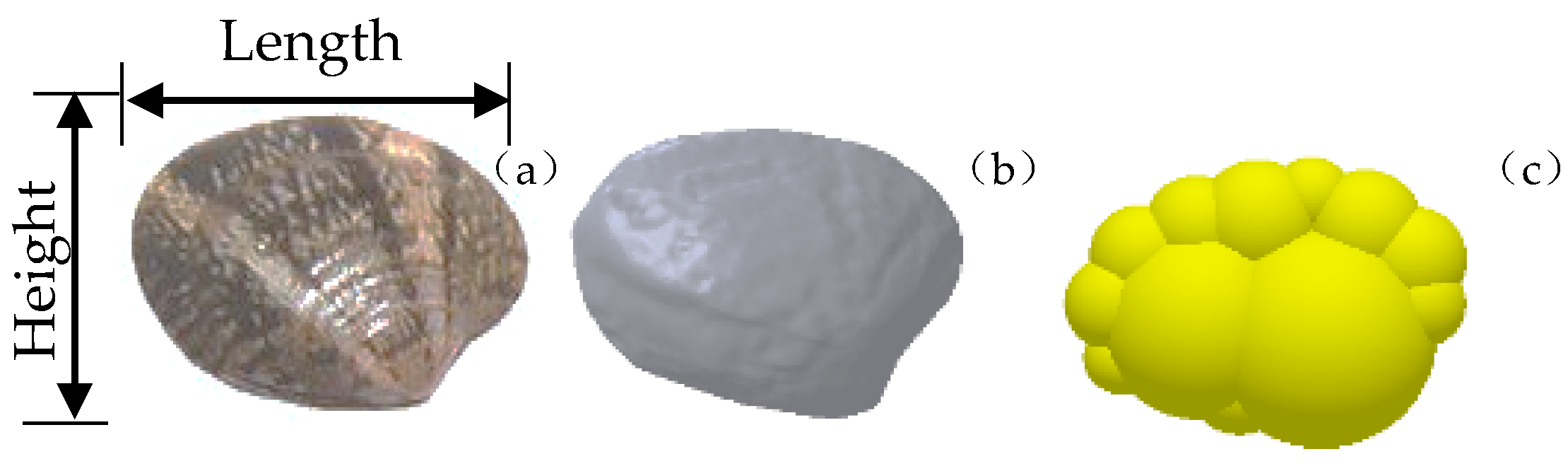
Due to the oval and irregular clam shape (Figure 1a), the clam three-dimensional (3D) shape (Figure 1b) was difficult to draw accurately, and so it was created by reverse engineering with a 3D scanner (Einscan-S, Shining3D, CHN) and Geomagic Studio software (Geomagic Studio 2016, Geomagic, Morrisville, NC, USA). Then the clam DEM shape (Figure 1c), based on the clam 3D shape, was filled with different size particles using the multi-sphere method (MSM) in EDEM software (EDEM 2018, DEM Solutions Ltd., Edinburgh, UK) [22]. The Hertz–Mindlin no-slip contact model, one of the most commonly employed contact models, was selected in EDEM [22,23,32]. The simulation contact parameters input in EDEM between the living clam and different contact materials were calibrated using the DEM simulation calibration approach.

Figure 1.
Clam (a), Clam 3D shape (b), and Clam DEM shape (c).
2.3. Measurement
2.3.1. The Static Friction Coefficient (μs)
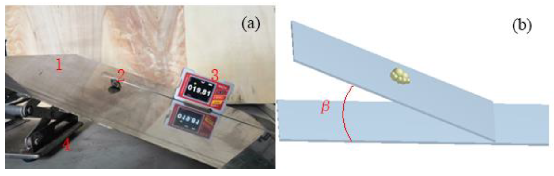
The particle–wall static friction coefficient (μs-pw) was determined using the inclined plate method [14,33]. The clam and digital inclinometer (DMI 410, Rion, Beijing, CHN) were placed on the inclined plate. One end of the inclined plate was fixed, and the other end ascended gradually with the lifting platform. When the clam began to slide down, the value of the inclination angle (β) was recorded by digital inclinometer and the μs-pw value was calculated (Figure 2a). Furthermore, the value of the particle-particle static friction coefficient (μs-pp) was difficult to measure directly and the μs-pp was determined in Section 2.4.2.
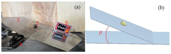
Figure 2.
Static friction coefficient calibration test: (a) direct measurement: 1 Wall; 2 Clam; 3 Inclinometer; 4 Lifting platform (b) DEM simulation test.
2.3.2. The Restitution Coefficient (e)
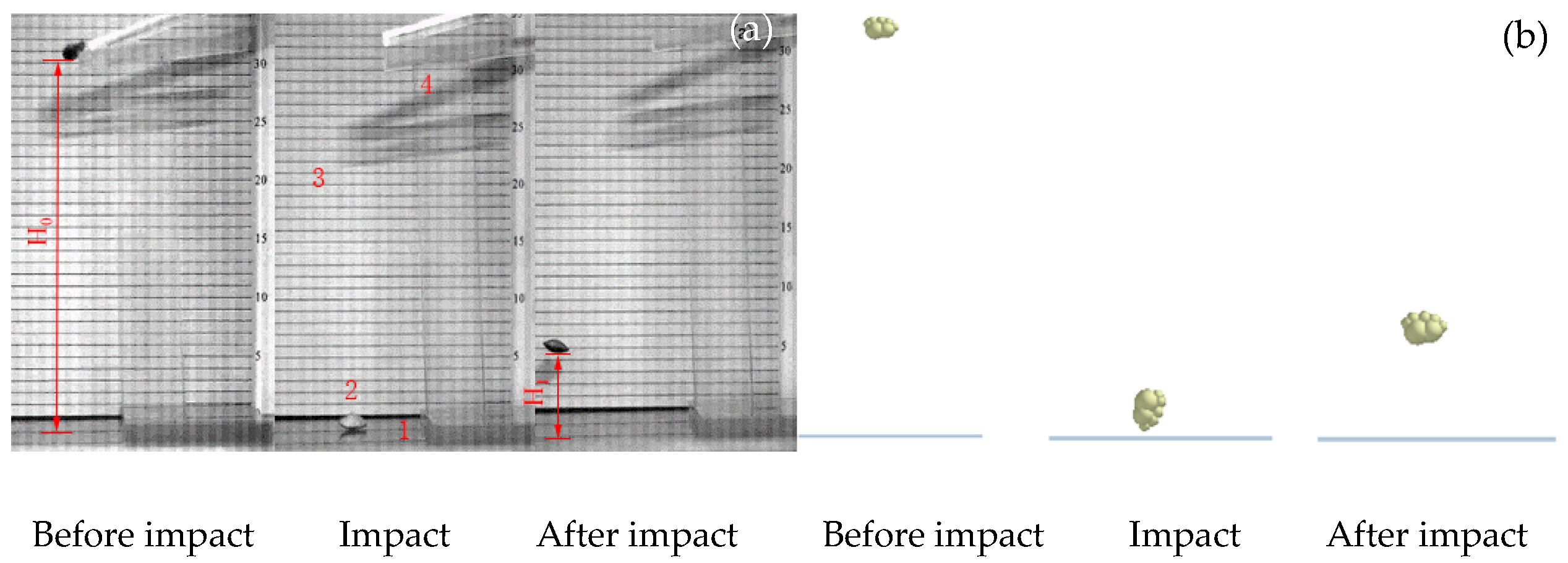
The restitution coefficient (e) was determined through drop tests [14]. SS, AC, and clam (the clams had been closely adhered to the SS plate) were used as the bottom plate, and the graph paper in 5 × 5 mm form was placed vertically as the experimental background to assist in measuring the height of rebounding. The clam fell freely from a height (H0) of 150 mm and initially rebounded to a maximum height (H1) [32,34]. The drop process was recorded with a high-speed video camera (Fastcamsa5, Photron, Tokyo, Japan) running at 1024 × 1024 pixels@1000 fps (Figure 3a). Then the video was converted into images using Matlab (Matlab 2014, Mathworks, Natick, MA, USA) to measure H1. The value of e was calculated by Equation (1).
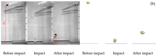
Figure 3.
Restitution coefficient calibration test: (a) direct measurement: 1 Wall; 2 Clam; 3 Graph paper; 4 Testbed (b) DEM simulation test.
2.3.3. The Static Repose Angle (θ)
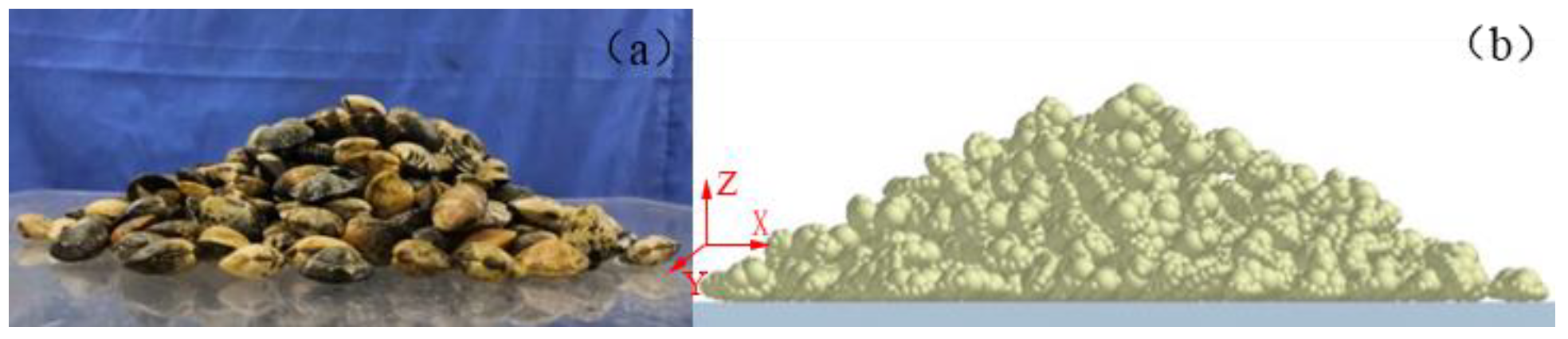
The static repose angle reflects the internal friction and scattering characteristics of granular materials. The clam static repose angle was measured by a lifting cylinder test [15]. A hollow cylinder (R = 50 mm, H = 350 mm) was placed vertically on the bottom plate, and 500 clams were poured into it. When the 500 clams in the hollow cylinder were in a stable state, the cylinder was elevated at a speed of 0.1 m/s [35]. The 500 clams were steadily deposited due to gravity, and the static repose angle of the four directions: X+, X−, Y+, Y− was measured with a digital inclinometer (Figure 4a).

Figure 4.
Clam stacking test: (a) direct measurement (b) DEM simulation test.
2.4. DEM Simulation Calibration
2.4.1. Calibration of the Fixed Contact Parameters
Calibration of the simulation contact parameters were carried out by EDEM. To keep the DEM simulation calibration results consistent with the direct measurements, the DEM simulation test was run as shown in Figure 2b, Figure 3b and Figure 4b. The DEM simulation results (simulation inclination angle (β’) and simulation rebound height (H1′)) were measured by EDEM analysis. The simulation contact parameters range was predicted by taking the direct measurements and extending the range at both ends. The simulation contact parameters range was divided into 5 groups, each group with a step length of 0.05, and they were respectively input into the DEM simulation calibration test [10]. Only one of the measured contact parameters in Section 2.4.1 and Section 2.4.2 (e, μs-pw) was taken as the variable, and the other simulation contact parameters (the simulation contact parameters without influence on the calibration test results) were set to 0 in each DEM simulation calibration test. For example, only the particle–wall simulation static friction coefficient (μ′s-pw) had an impact on the β’ results in the DEM simulation calibration test, so the remaining contact parameters, apart from μ′s-pw, were set to 0. The DEM simulation test data were entered into Original software (Original2019, Origin Lab, Northampton, MA, USA) to obtain the quadratic polynomial fitting curve and equation. The accuracy of the quadratic polynomial fitting equation was evaluated by the R2 value. Subsequently, the results of direct measurement parameters (β and H1) were brought into the quadratic polynomial fitting equation as the target values to calculate and calibrate the simulation contact parameters. The calibrated simulation contact parameters were re-entered into the EDEM software, and the DEM simulation test was repeated to acquire the results. The relative error (δ) between the DEM simulation test results and direct measurements was calculated to verify the accuracy of the simulation contact parameters.
2.4.2. Response Surface Simulation Test
As the particle–wall (μr-pw) and particle-particle (μr-pp) rolling friction coefficients and the particle-particle static friction coefficient (μs-pp) were difficult to measure directly, the simulation contact parameters (particle–wall simulation rolling friction coefficient (μ′r-pw), particle-particle simulation static friction coefficient (μ′s-pp), particle-particle simulation rolling friction coefficient (μ′r-pp)) could not be obtained by the method in Section 2.4.1. Therefore, response surface methodology (RSM) was used to find the best combination of simulation contact parameters. Box–Behnken Design (BBD), an RSM method, was applied. The calibrated simulated contact parameters in Section 2.4.1 were input into EDEM for a clam stacking simulation pre-test, and the value range of the other uncalibrated simulation contact parameters (μ′r-pp-ss, μ′s-pp-ss, μ′r-pw-ss, μ′r-pp-ac, μ′s-pp-ac, μ′r-pw-ac) was estimated. Then a 3 factor and 3 level (high (+1), medium (0), and low (−1)) BBD test was applied for the numerical design [21], and the simulation repose angles of Clam-SS (θ’ss) and Clam-AC (θ’ac) were evaluated as the response index.
The analysis of variance (ANOVA) was applied to assess the main effects and interactions. A multiple regression equation, without non-significant factors, was obtained based on ANOVA results of BBD tests. The directly measured clam static repose angle was placed as the target value into the multiple regression equation, and the optimal combinations of the other simulation contact parameters (μ′r-pw, μ′s-pp, μ′r-pp) under different contact parameters were calculated. All the calibrated simulation contact parameters were input into the EDEM software for repeating the simulation lifting cylinder test, and the simulation static repose angle was measured. Additionally, by calculating the clam static repose angle relative error (δa) between the measured and simulated values, the accuracy of the clam DEM model was verified.
2.5. Clam DEM Model Seeding Verification Test
The accuracy of the calibrated clam DEM model was evaluated in a clam seeding verification test by comparing the average error of the variation coefficient between the direct and simulated seeding tests. Taking the seeding wheel rotation speed as the variable, a clam seeding test of the five groups was conceived. The clam feeding speed of the blanking hopper was 0.2 kg s−1, and the conveyor belt speed (i.e., seeding equipment advancing speed) was 0.75 m s−1 in the test. In each test, the weight of clams discharged onto conveyor belts (i.e., clam seeding area) by seeding wheels on five continuous grids was measured. The clam seeding equipment, designed and used in direct seeding tests, consisted of a blanking hopper, a seeding tray, and a seeding wheel. The seeding tray and wheel were manufactured through 3D printing, and the inner wall of the seeding wheel adhered to AC plates (Figure 5a). The 3D seeding equipment model, clam DEM model, and the AC plate were imported into EDEM software for the seeding simulation test (Figure 5b). The variation coefficient was calculated according to Equations (2)–(4). The testing protocol of the DEM simulation and realistic seeding tests were the same:
where CV was the variation coefficient, %; S was the standard deviation, g; n was the grid number; M0 was the average feed weight collected by the grid in the collection domain, g; Mi was the feed weight collected in i computing grid, g.
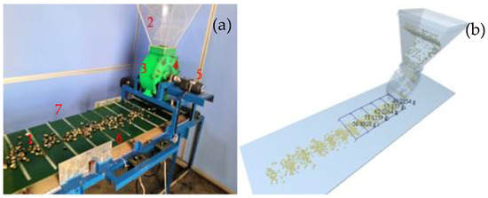
Figure 5.
Clam seeding verification test: (a) direct seeding test: 1 Clam; 2 Blanking hopper; 3 Seeding tray; 4 Seeding wheel; 5 Motor; 6 Conveyor belt; 7 Grid (b) DEM simulation seeding test.
2.6. Statistical Analysis
Each direct measurement group and DEM simulation calibration test were repeated 10 times to calculate the mean value. The response surface test results were calculated by Design Expert software (Design expert 10, Stat-Ease, Minneapolis, MN, USA), with a significant impact level of 95% (p < 0.05), and a highly significant impact level of 99% (p < 0.01).
3. Results and Discussion
3.1. The Static Friction Coefficient (μs)
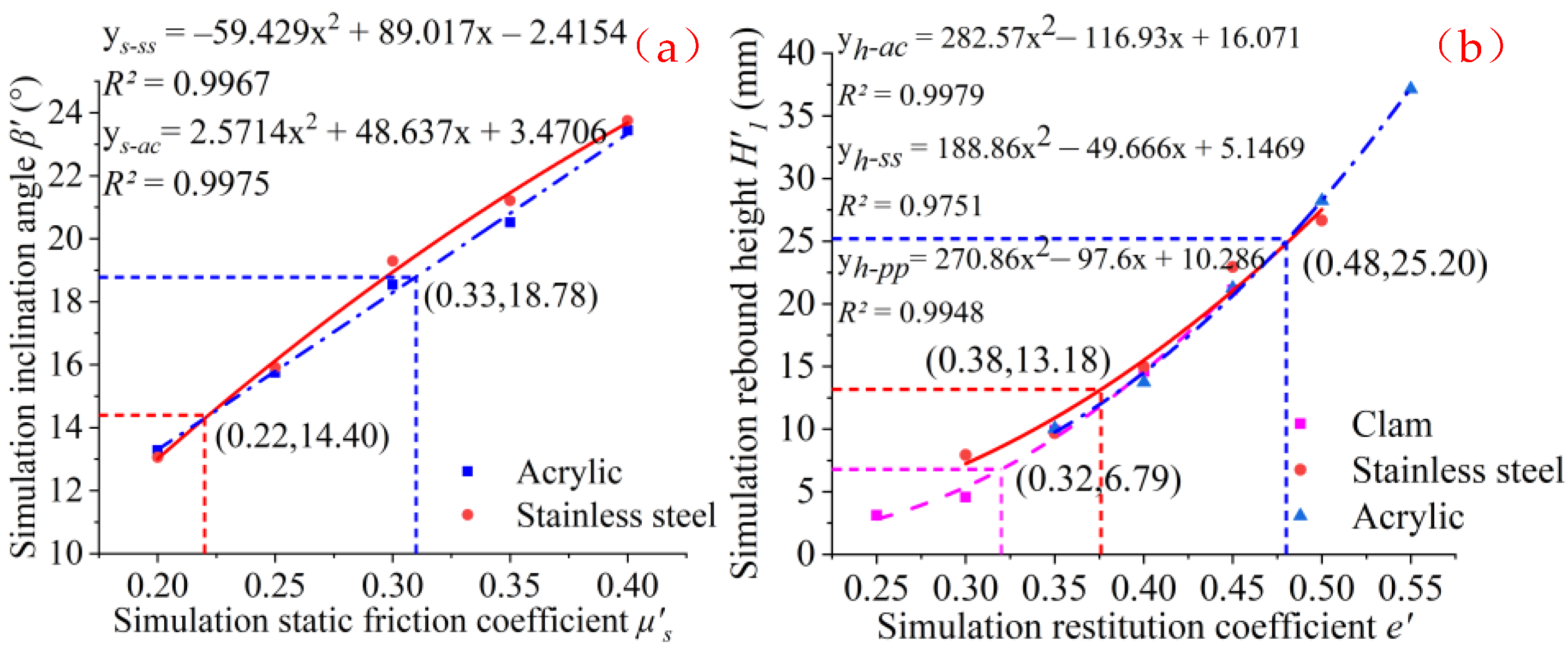
The direct measurement results of β and μs-pw between clam and SS, and AC are shown in Table 2. Due to a μs-pw-ss and μs-pw-ac of 0.26 and 0.34, respectively, the resulting μ′s-pw prediction range was 0.20–0.40. The quadratic polynomial fitting curve and equation ys-ss, ys-ac based on the DEM simulation test were fitted and are shown in Figure 6a. The coordinates obtained by virtual line marking in Figure 6a are the simulation contact parameters (μ′s-pw) and their test results (β’) in the DEM simulation calibration tests.
Table 2.
Particle–wall coefficient of static friction (μs-pw) for SS and AC.
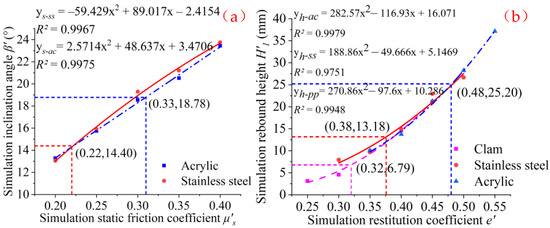
Figure 6.
DEM simulation calibration fitting curve and equation of relation (a) simulation static friction coefficient and inclination angle (b) simulation restitution coefficient and rebound height. In the Figure, the ordinate of the coordinates located by the dotted line represents the realistic value of direct measurements, and the abscissa represents the calculated simulation contact parameters.
As shown in Table 2, the directly measured βac and μs-pw-ac were 1.31 times more than the βss and μs-pw-ss, and a similar result occurred in the DEM simulation test. Due to the AC surface roughness, the static friction between clam and AC was sizeable. Therefore, in the clam seeding equipment design, AC would be the most appropriate material when increasing friction was required. For example, to avoid the clams dropping too quickly and causing congestion at the outlet of the dropping hopper, it would be necessary to add a high friction guide plate in the blanking hopper; hence, AC would be the recommended material. Conversely, SS would be the obvious choice when friction needs to be minimized.
The simulation value μ′s-pw was significantly smaller than μs-pw (as shown in Table 2). The reason may be that the clam DEM model was composed of smooth particles; however, clams have a growth line on their surface that grows with increasing clam size. As the clam growth lines gradually deepened, the surface roughness and the static friction coefficient (μs) also gradually increased, which concurs with previous studies that suggest that the larger the clam size, the greater the static friction coefficient is [31]—hence why the μs-pw was larger than μ′s-pw, as also in the calibration case of panax notoginseng seeds [36].
Furthermore, the value of the inclination angle relative error (δa) between β’ and β included: δa-ss = 4.0%, δa-ac = 1.8%, respectively. It indicated that the simulation inclination angle was consistent with the direct measurements. The DEM calibration test results of the static friction coefficient were accurate, which could then be applied to the clam simulation study.
3.2. The Coefficient of Restitution (e)
The coefficients of restitution (e) for SS, AC, and Clam are shown in Table 3. According to the calculated restitution coefficient results: epw-ss = 0.30, epp = 0.21, epw-ac = 0.41, the predicted range of the simulation restitution coefficient was 0.25–0.55. Figure 6b shows the relationship between the simulation restitution coefficient (e’) and rebound height (H’1) in the fitting curve and equation yh-ss, yh-ac, yh-pp. The coordinates obtained by virtual line marking in Figure 6b are the simulation contact parameters (e’) and their test results (H1’) in the DEM simulation test.
Table 3.
The coefficient of restitution (e) for SS, AC, and Clam.
As illustrated in Table 3, the e varied in direct measurement, and the epp < epw-ss < epw-ac. The lower the restitution coefficient, the lower rebound height is. In the process of clam seeding, when clams fall into the groove on the seeding wheel through the bottom of the blanking hopper, they rebound. When the rebound height of the clams is higher than the depth of the groove, the clams are crushed by the seeding wheel and the seeding traying. To avoid this affecting, SS, with a small restitution coefficient, should be selected as the surface contact material of the seeding wheel. AC with a high restitution coefficient would be an appropriate contact material if the impact of rebound height was negligible and the clam breakage rate could be reduced by modifying the equipment structure.
Additionally, the e’ was greater than in Table 3; specifically, the e’pw-ac was 0.48, which is 17.1% larger than the e’pw-ac. This may be because the center of gravity of the clam is different from that of its DEM model. The clam is composed of an external shell, internal flesh, and a small amount of water, which are heterogeneous granular materials. Due to the different shapes and water content between clams, the center of gravity of each clam also varies. Therefore, when each clam lands on the bottom plate, the impact position and rebound height are different. However, the clam DEM model in the simulated drop test was filled with solid homogeneous granular materials, and the gravity center and impact position were more fixed than the living clam. Therefore, the direct measurement rebound height was significantly lower than in the DEM simulation test result.
The rebound height relative error (δH1) between H’1 and H1 was: 1.7%, 1.7%, 2.1%, respectively. The DEM simulation test result was similar to the direct measurement, which could effectively replace the realistic drop test.
3.3. Response Surface Simulation Test and ANOVA
The results of the directly measured static repose angles of Clam-SS (θss) and Clam-AC (θac) were θss = 31.75°, θac = 38.07°. The range of the simulation contact parameters was predicted by a clam stacking simulation pre-test. With an SS wall, the simulation rolling coefficient of Clam-Clam (μ′r-pp) was in the range of 0.14−0.22, the simulation statics coefficient of Clam-Clam (μ′s-pp) was in the range of 1.04−1.12, and the rolling coefficient of Clam-SS (μ′r-pw-ss) was in the range of 0.14−0.22. The simulation contact parameter range for an AC wall was also predicted. The factors and levels from the response surface simulation test are shown in Table 4.
Table 4.
Factors and levels.
In this study, 17 experiments were carried out to find the best combination of simulation contact parameters and to study the effect of the μ′r-pp, μ′s-pp, and μ′r-pw on the clam simulation static repose angle, based on the BBD method [37]. The corresponding simulation results are shown in Table 5.
Table 5.
Experimental scheme and response results based on the BBD method.
In ANOVA, the p-value represents the significance of the factors. The F-value represents the primary and secondary order of influence that the factors had on the response. The larger the F-value, the stronger the influence on the response was. The ANOVA results for the quadratic polynomial model are shown in Table 6. With an SS bottom plate, the simulation contact parameters: μ′r-pp, μ′s-pp, μ′r-pw, μ′r-pp μ′s-pp, μ′r-ppμ′r-pw, μ′s-pp2, and μ′r-pp 2 showed highly significant influence (p < 0.01), whereas μ′s-ppμ′r-pw and μ′r-pw2 showed insignificant influence. The influence order of the factors was μ′s-pp > μ′s-pp2 > μ′r-pp > μ′r-ppμ′s-pp > μ′r-pp2 > μ′r-ppμ′r-pw > μ′r-pw > μ′r-pw2 > μ′s-ppμ′r-pw. With an AC bottom plate, the simulation contact parameters: μ′r-pp, μ′r-pw2 showed highly significant influence and μ′s-pp, μ′s-ppμ′r-pw, μ′s-pp2 showed significant influence (p < 0.05), whereas μ′r-ppμ′r-pw and μ′r-pw2 showed insignificant influence. The influence order of the factors was μ′r-pp > μ′r-pw2 > μ′s-pp > μ′s-pp2 > μ′s-ppμ′r-pw > μ′r-ppμ′s-pp > μ′r-pp2 > μ′r-pw > μ′r-ppμ′r-pw.
Table 6.
ANOVA results of BBD tests.
In both SS and AC regression models, the parameters such as the lack of fit p value, the coefficient of variation (CV), determination coefficient (Rs2), correction determination coefficient (Adj−Rs2), and the Adeq−Precision demonstrated good predictability with the multiple regression equation (Equations (5) and (6)).
Some simulation contact parameters, obtained through the multiple regression Equations (5) and (6), included: μ′r-pp-ss = 0.33, μ′r-pp-ac = 0.20, μ′s-pp-ss = 1.25, μ′s-pp-ac = 1.12, μ′r-pw-ss = 0.34, μ′r-pw-ac = 0.17. The clam simulation static repose angles included: θ’ss = 31.55° and θ’ac = 37.90°, and the relative error between θ and θ’ included: δa-ss = 0.04% and δa-ac = 0.06%, respectively. As there was no obvious difference between the DEM simulation test and the direct measurement results; the accuracy of the clam simulation contact parameters was high. Therefore, the clam DEM model could be used for EDEM simulation for clam seeding.
The static repose angle in the stacking test was determined as θss < θac by comparing the direct measurement AC and SS results. This may be because the roughness of the AC surface is greater than that of smoother SS. The larger the μs-pw-ac, the larger the θac with the AC bottom plate is. It could be inferred that the μs-pw, μs-pw, μr-pp, and μs-pp have a significant effect on the static repose angle of clams, as illustrated in Table 6. Consequently, it could be inferred that the clam contact parameters μs-pw, μr-pp, μs-pp had a significant effect on the application of the clam DEM model, and the response surface simulation test conclusions were similar to the published result [11]. Therefore, the influence of μs-pw, μr-pp, and μs-pp on the seeding effect should be fully considered when designing and optimizing clam seeding equipment.
3.4. Clam Seeding Verification Test
As shown in Figure 7, as the rotation speed of the seeding wheel increases to 30 r min−1, the δt value and the realistic and simulated values of the coefficient of variation decrease; however, when this rotation speed increases from 30 r min−1 to 45 r min−1, the said values start to increase. When the seeding wheel speed was around 30 r min−1, all the variation coefficients were at their lowest values. The smaller the variation coefficient, the more uniform the distribution of clams is. Therefore, an optimal working rotation speed of around 30 r min−1, which is the best matching relationship with the feeding speed and the equipment advancing speed in this study, for clam seeding equipment is recommended. With a slower seeding wheel rotation speed, the seeding continuity was reduced, consequently increasing the clam seeding variation coefficient. On the contrary, when the rotation speed of the seeding wheel was higher, the groove of the seeding wheel directly below the clam blanking hopper was not full; the groove had already rotated away. Therefore, the clam seeding variation coefficient and test error were large. When the seeding wheel rotation speed was 30 r min−1, the feeding speed and advancing speed were more appropriate. Moreover, the verification results were also helpful in the design and optimization of the clam seeding equipment and could effectively help to understand the motion state of clams for future designers, whilst providing a technical reference.
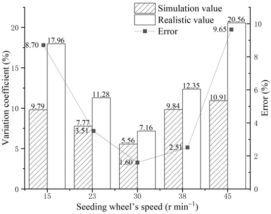
Figure 7.
Clam seeding verification test.
As shown in Figure 7, the minimum and maximum values of the variation coefficient error (δt) were 9.65%, and 1.60%, and the average value of δt was 4.98%. The results showed that the clam seeding realistic and simulated tests were highly similar, so it could be inferred that the accuracy of the clam DEM model was high. Therefore, the clam seeding simulation could effectively simulate actual clam seeding.
4. Conclusions
In this study, based on the clam DEM particle shape, the clam simulation contact parameters and a clam seeding verification test were calibrated and analyzed by DEM. The conclusions are as follows:
- (1)
- The clam simulation contact parameters of different contact materials (SS and AC) were determined by a DEM simulation calibration test. When SS was the contact material, the simulation contact parameters in the calibrated set included: μ′s-pw-ss = 0.22, e’pw-ss = 0.38, e’pp = 0.32, μ′r-pp-ss = 0.33, μ′s-pp-ss = 1.25, μ′r-pw-ss = 0.34. Similarly, with AC, μ′s-pw-ac =0.31, e’pw-ac = 0.48, e’pp = 0.32, μ′r-pp-ac = 0.20, μ′s-pp-ac = 1.12, μ′r-pw-ac = 0.17.
- (2)
- The accuracy of the simulation contact parameters (μ′s-pp, μ′r-pp, μ′s-pw) was simultaneously verified, and they were found to have a significant effect on the clam DEM model.
- (3)
- Through comparing the results of the clam realistic and simulated seeding tests, it was verified that the accuracy of the clam DEM model was high, and therefore it could be applied for clam seeding DEM simulation and equipment design in the future.
Author Contributions
Methodology, W.L.; formal analysis, Q.Z.; data curation, H.Z.; writing—original draft preparation, H.L.; writing—review and editing, G.M.; supervisor, G.Z.; funding acquisition, X.L. All authors have read and agreed to the published version of the manuscript.
Funding
This research was funded by The National Key R&D Program of China, grant number 2019YFD0900701.
Institutional Review Board Statement
Not applicable.
Informed Consent Statement
Not applicable.
Data Availability Statement
Not applicable.
Conflicts of Interest
The authors declare no conflict of interest.
References
- Ye, L.H.; Cai, S.L.; Chen, H.B.; Wu, J.N.; Liu, Z.Y.; Su, Y.C. Study of processing technology for leisure food of ready-to-eat Ruditapes philippinarum. J. Fish. Res. 2016, 38, 363–371. [Google Scholar]
- Yuan, H.; Shen, H.; Wang, L.B.; Shi, L.K. Ecological Culture Technology of Ruditapes Philippines Beach. Fish. Sci. Technol. Inf. 2014, 41, 54–56. [Google Scholar]
- Zeng, Z.W.; Ma, X.; Cao, X.L.; Li, Z.H.; Wang, X.C. Critical Review of Applications of Discrete Element Method in Agricultural Engineering. Trans. Chin. Soc. Agric. Mach. 2021, 52, 1–20. [Google Scholar]
- Cundall, P.A.; Strack, O. A discrete numerical model for granular assemblies. Géotechnique 2008, 30, 331–336. [Google Scholar] [CrossRef] [Green Version]
- Ma, Z.; Li, Y.M.; Xu, L.Z.; Chen, J.; Zhao, Z.; Tang, Z. Dispersion and migration of agricultural particles in a variable-amplitude screen box based on the discrete element method. Comput. Electron. Agric. 2017, 142, 173–180. [Google Scholar] [CrossRef]
- Wang, Q.R.; Mao, H.P.; Li, Q.L. Modelling and simulation of the grain threshing process based on the discrete element method. Comput. Electron. Agric. 2020, 11, 178. [Google Scholar] [CrossRef]
- Zeng, Z.W.; Chen, Y. Simulation of straw movement by discrete element modelling of straw-sweep-soil interaction. Biosyst. Eng. 2019, 180, 25–35. [Google Scholar] [CrossRef]
- Xie, H.F.; Gao, G.H.; Tian, B.X.; Li, B.W.; Zhang, S.; Huang, J. Optimization of Potato Soil Transportation Separation Mechanism Based on Discrete Element Method and TRIZ Theory. J. Phys. Conf. Ser. 2019, 1267. [Google Scholar] [CrossRef]
- Liu, W.Z.; HE, J.; Li, H.W.; Li, X.Q.; Zheng, K.; Wei, Z.C. Calibration of Simulation Parameters for Potato Minituber Based on EDEM. Trans. Chin. Soc. Agric. Mach. 2018, 49, 125–135. [Google Scholar]
- Grima, A.P.; Wypych, P.W. Investigation into calibration of discrete element model parameters for scale-up and validation of particle–structure interactions under impact conditions. Powder Technol. 2011, 212, 198–209. [Google Scholar] [CrossRef]
- Liu, F.Y.; Zhang, J.; Li, B.; Chen, J. Calibration of parameters of wheat required in discrete element method simulation based on repose angle of particle heap. Trans. Chin. Soc. Agric. Eng. 2016, 32, 247–253. [Google Scholar]
- Coetzee, C.J. Review: Calibration of the discrete element method. Powder Technol. 2017, 310, 104–142. [Google Scholar] [CrossRef]
- Shi, L.R.; Ma, Z.T.; Zhao, W.Y.; Yang, X.P.; Sun, B.G.; Zhang, J.P. Calibration of simulation parameters of flaxed seeds using discrete element method and verification of seed-metering test. Trans. Chin. Soc. Agric. Eng. 2019, 35, 25–33. [Google Scholar]
- González-Montellano, C.; Fuentes, J.M.; Ayuga-Téllez, E.; Ayuga, F. Determination of the mechanical properties of maize grains and olives required for use in DEM simulations. J. Food Eng. 2012, 111, 553–562. [Google Scholar] [CrossRef]
- Rackl, M.; Hanley, K.J. A methodical calibration procedure for discrete element models. Powder Technol. 2017, 307, 73–83. [Google Scholar] [CrossRef] [Green Version]
- Boikov, A.V.; Savelev, R.V.; Payor, V.A. DEM Calibration Approach: Design of experiment. J. Phys. Conf. Ser. 2018, 1015, 032017. [Google Scholar] [CrossRef]
- Wang, L.J.; Zhou, W.X.; Ding, Z.J.; Li, X.X.; Zhang, C.G. Experimental determination of parameter effects on the coefficient of restitution of differently shaped maize in three-dimensions. Powder Technol. 2015, 284, 187–194. [Google Scholar] [CrossRef]
- Mousaviraad, M.; Tekeste, M.Z.; Rosentrater, K.A. Calibration and Validation of a Discrete Element Model of Corn Using Grain Flow Simulation in a Commercial Screw Grain Auger. Trans. ASABE 2017, 60, 1403–1415. [Google Scholar] [CrossRef] [Green Version]
- Pasha, M.; Hare, C.; Ghadiri, M.; Gunadi, A.; Piccione, P.M. Effect of particle shape on flow in discrete element method simulation of a rotary batch seed coater. Powder Technol. 2016, 296, 29–36. [Google Scholar] [CrossRef] [Green Version]
- Coetzee, C. Calibration of the discrete element method: Strategies for spherical and non-spherical particles. Powder Technol. 2020, 364, 851–878. [Google Scholar] [CrossRef]
- Santos, K.G.; Campos, A.; Oliveira, O.S.; Ferreira, L.V.; Francisquetti, M.C.; Barrozo, M. DEM simulations of dynamic angle of repose of acerola residue: A parametric study using a response surface technique. In Proceedings of the XX Congresso Brasileiro de Engenharia Química, João Pessoa, Brazil, 7 December 2015. [Google Scholar]
- Zhao, Z.; Wu, Y.F.; Yin, J.J.; Tang, Z. Monitoring method of rice seeds mass in vibrating tray for vacuum-panel precision seeder. Comput. Electron. Agric. 2015, 114, 25–31. [Google Scholar]
- Zhang, S.; Tekeste, M.Z.; Li, Y.; Gaul, A.; Zhu, D.; Liao, J. Scaled-up rice grain modelling for DEM calibration and the validation of hopper flow. Biosyst. Eng. 2020, 194, 196–212. [Google Scholar] [CrossRef]
- Boac, J.M.; Ambrose, R.P.K.; Casada, M.E.; Maghirang, R.G.; Maier, D.E. Applications of Discrete Element Method in Modeling of Grain Postharvest Operations. Food Eng. Rev. 2014, 6, 128–149. [Google Scholar] [CrossRef] [Green Version]
- Ghodki, B.M.; Patel, M.; Namdeo, R.; Carpenter, G. Calibration of discrete element model parameters: Soybeans. Comput. Part. Mech. 2018, 6, 3–10. [Google Scholar] [CrossRef]
- Shi, L.R.; Sun, W.; Zhao, W.Y.; Yang, X.P.; Feng, B. Parameter determination and validation of discrete element model of seed potato mechanical seeding. Trans. Chin. Soc. Agric. Eng. 2018, 34, 35–42. [Google Scholar]
- Liao, Y.T.; Wang, Z.T.; Liao, Q.X.; Wan, X.Y.; Zhou, Y.; Liang, F. Calibration of Discrete Element Model Parameters of Forage Rape Stalk at Early Pod Stage. Trans. Chin. Soc. Agric. Mach. 2020, 51, 236–243. [Google Scholar]
- Wu, M.C.; Cong, J.L.; Yan, Q.; Zhu, T.; Peng, X.Y.; Wang, Y.S. Calibration and experiments for discrete element simulation parameters of peanut seed particles. Trans. Chin. Soc. Agric. Eng. 2020, 36, 30–38. [Google Scholar]
- Hao, J.J.; Long, S.F.; Li, H.; Jia, Y.L.; Ma, Z.K.; Zhao, J.G. Development of discrete element model and calibration of simulation parameters for mechanically-harvested yam. Trans. Chin. Soc. Agric. Eng. 2019, 35, 34–42. [Google Scholar]
- Mu, G. Research on Mechanical Properties Tests of Clam and Key Issues of Dredge Machinery. Ph.D. Thesis, Dalian University of Technology, Dalian, China, 2019. [Google Scholar]
- Liu, W.B.; Zhang, H.B.; Li, X.C.; Zhang, G.C.; Zhang, Q.; Qu, S.G.; Gao, J.Y.; Fan, B.; Mu, G. Analysis of biomechanical properties of juvenile Manila clam for mechanization sowing. J. Dalian Ocean. Univ. 2020, 35, 455–461. [Google Scholar]
- Cabiscol, R.; Finke, J.H.; Kwade, A. Calibration and interpretation of DEM parameters for simulations of cylindrical tablets with multi-sphere approach. Powder Technol. 2018, 327, 232–245. [Google Scholar] [CrossRef]
- Ramírez-Gómez, Á.; Gallego, E.; Fuentes, J.M.; González-Montellano, C.; Ayuga, F. Values for particle-scale properties of biomass briquettes made from agroforestry residues. Particuology 2014, 12, 100–106. [Google Scholar] [CrossRef]
- González-Montellano, C.; Ramírez, Á.; Gallego, E.; Ayuga, F. Validation and experimental calibration of 3D discrete element models for the simulation of the discharge flow in silos. Chem. Eng. Sci. 2011, 66, 5116–5126. [Google Scholar] [CrossRef]
- Yan, Z.; Wilkinson, S.K.; Stitt, E.H.; Marigo, M. Discrete element modelling (DEM) input parameters: Understanding their impact on model predictions using statistical analysis. Comput. Part. Mech. 2015, 2, 283–299. [Google Scholar] [CrossRef] [Green Version]
- Yu, Q.; Liu, Y.; Chen, X.; Sun, K.; Lai, Q. Calibration and Experiment of Simulation Parameters for Panax notoginseng Seeds Based on DEM. Trans. Chin. Soc. Agric. Mach. 2020, 51, 123–132. [Google Scholar]
- Boikov, A.V.; Savelev, R.V.; Payor, V.A.; Vasileva, N.V. DEM calibration approach: Orthogonal experiment. J. Phys. Conf. Ser. 2019, 1210, 012025. [Google Scholar] [CrossRef]


Publisher’s Note: MDPI stays neutral with regard to jurisdictional claims in published maps and institutional affiliations. |
© 2021 by the authors. Licensee MDPI, Basel, Switzerland. This article is an open access article distributed under the terms and conditions of the Creative Commons Attribution (CC BY) license (https://creativecommons.org/licenses/by/4.0/).