Abstract
Improving agricultural productivity is essential due to rapid population growth, making early detection of crop diseases crucial. Although deep learning shows promise in smart agriculture, practical applications for identifying wheat diseases in complex backgrounds are limited. In this paper, we propose CropNet, a hybrid method that utilizes Red, Green, and Blue (RGB) imaging and a transfer learning approach combined with shallow convolutional neural networks (CNN) for further feature refinement. To develop our customized model, we conducted an extensive search for the optimal deep learning architecture. Our approach involves freezing the pre-trained model for feature extraction and adding a custom trainable CNN layer. Unlike traditional transfer learning, which typically uses trainable dense layers, our method integrates a trainable CNN, deepening the architecture. We argue that pre-trained features in transfer learning are better suited for a custom shallow CNN followed by a fully connected layer, rather than being fed directly into fully connected layers. We tested various architectures for pre-trained models including EfficientNetB0 and B2, DenseNet, ResNet50, MobileNetV2, MobileNetV3-Small, and Inceptionv3. Our approach combines the strengths of pre-trained models with the flexibility of custom architecture design, offering efficiency, effective feature extraction, customization options, reduced overfitting, and differential learning rates. It distinguishes itself from classical transfer learning techniques, which typically fine-tune the entire pre-trained network. Our aim is to provide a lightweight model suitable for resource-constrained environments, capable of delivering outstanding results. CropNet achieved 99.80% accuracy in wheat disease detection with reduced training time and computational cost. This efficient performance makes CropNet promising for practical implementation in resource-constrained agricultural settings, benefiting farmers and enhancing production.
1. Introduction
The foundation of our society is built upon agriculture, which sustains and feeds billions of people worldwide. As the global population continues to grow, maintaining a stable and secure food supply has become increasingly crucial. Agriculture not only plays a fundamental role in providing sustenance but also promotes economic development and creates job opportunities, benefiting millions worldwide. Wheat is a highly consumed crop globally, with annual per capita consumption surpassing 50 kg in 102 countries [1]. However, addressing plant diseases is imperative, as they significantly impact crop yields and food production. A large portion of crop production is lost to diseases every year [2]. Hence, timely adoption of protective measures stands as a highly effective approach to prevent crop diseases and reduce losses. Visual examination has traditionally been the primary diagnostic technique for wheat cultivation. However, this method is becoming increasingly challenging as it demands significant time and effort from both farmers and pathologists to accurately measure infection levels. Manual detection of wheat diseases is not only time-intensive, costly, and resource-intensive, but also requires expert knowledge, often leading to poor performance and incorrect diagnoses. In response to these challenges, researchers and farmers have begun seeking accurate, rapid, automated, and cost-effective methods for disease detection. Improvement in computer vision and machine learning (ML) have enabled the development of computerized models capable of accurately detecting plant diseases. Several studies have used ML techniques to identify and detect plant diseases [3,4,5]. However, traditional ML algorithms often require domain experts to specify the majority of essential features, which can complicate data processing and pattern recognition. Deep learning (DL) techniques have recently enhanced machine learning by autonomously learning and extracting crucial features from data, thereby enabling more accurate pattern recognition. CNNs are among the most popular technologies in DL for quickly identifying crop diseases. For DL models to effectively learn and make decisions, a large dataset is essential. Hence, the importance of transfer learning arises, which involves transferring knowledge from one concept to another. Transfer learning plays a significant role in this scenario. In transfer learning, a new model is initialized using a previously trained model. Furthermore, farmers face numerous practical challenges, including limited access to high-end computing resources and stable internet connections in rural areas. These challenges have motivated this work to develop a model effective for detecting diseases in real-time, which can be beneficial to farmers in isolated areas. These constraints underscore the necessity for lightweight models that demand minimal computational resources, ensuring effective deployment in environments where such resources are scarce. Moreover, lightweight models enable real-time decision-making, crucial in disease detection scenarios where early intervention can prevent significant crop losses. By processing images directly on the field, these models empower farmers to make immediate decisions based on accurate diagnoses, enhancing overall crop management practices. Additionally, the cost-effectiveness of lightweight models, coupled with their scalability, makes them accessible to small-scale farmers and agricultural communities with limited financial resources. By deploying lightweight models across a wide range of farms and regions, the benefits of automated disease detection become more readily available, ultimately improving crop yields and ensuring food security on a broader scale. In the literature, only a limited number of studies employ DL/ML algorithms for wheat disease identification, with few offering lightweight models that are applicable for deployment in farm environments. Moreover, enhancing disease recognition rates is crucial to increase wheat farming globally. Therefore, it is essential to pursue further research in this area. This study effectively identifies wheat diseases from a limited dataset through a hybrid deep learning approach. It utilizes transfer learning models for feature extraction and employs CNNs or deep neural networks (DNNs) for classification. Additionally, it analyzes the effectiveness of different hybrid algorithms when integrated with CNNs and DNNs. This study also assesses the proposed approach’s performance across various standard metrics and compares it with other cutting-edge methods. Additionally, the model’s compact size and adaptability for deployment in limited and constrained environments make it suitable for farm settings, where devices often have limited processing power. The main contributions of this paper are outlined below:
- We introduced a hybrid model for wheat disease detection using a small dataset, leveraging both a deep learning framework and transfer learning. Our approach was tested on complex images captured in realistic growth scenarios with diverse backgrounds;
- We evaluated the proposed model by applying a range of diverse metrics, like accuracy, precision, recall, F1-score, and confusion matrix;
- We justified our model by distinguishing it from other cutting-edge models through the use of precision, recall, and accuracy;
- We validated the lightweight nature of our model and its suitability for deployment on edge devices by evaluating its size and trainable parameters in comparison to other cutting-edge research.
This paper is organized as follows. Section 2 and Section 3 review relevant studies on plant disease detection and gives some necessary background information, while Section 4 outlines the methodology employed in this research. Section 5 details the results obtained from the proposed approach. Section 6 offers a detailed comparison and discussion of the findings, and Section 7 wraps up the paper with a conclusion.
2. Related Works
Crop health is essential for ensuring agricultural production and food security. Diseases targeting plant leaves are a major threat to crop cultivation. To reduce yield losses and maintain crop health, it is essential to identify and treat these diseases early on. In current studies, efficient methods have been introduced to diagnose plant diseases using DL and ML approaches. Prodeep et al. recently published a study where various popular CNN architectures were compared to identify plant diseases in multi-label and multi-class classification tasks. The authors demonstrated that the EfficientNet model achieved better results. Meanwhile, when the model was evaluated on standard datasets, it showed poor performance [6]. Jouini et al. offered a lightweight deep CNN model to identify wheat leaf diseases [7]. The authors developed a model to detect wheat leaf diseases using RBG images with complex backgrounds. In their research, they began by experimenting with different CNN architectures, including DenseNet, ResNet, Inception3, EfficientNet and MobileNetV2, along with various optimizers and learning rates. They achieved a test accuracy of 94% with MobileNetV2 and a model size of 30 MB; they also demonstrated the efficacy of real-time disease detection in wheat, especially in environments with limited resources. However, the authors worked with a small and imbalanced dataset, consisting of 2092 images. A larger balanced dataset would likely improve the accuracy of this work. To detect and prevent grapevine diseases, the authors of this study presented AI GrapeCare, a user-friendly DL software. Their approach combined various DNN and image analysis techniques to achieve high accuracy. Their best-performing model, based on VGG16 with data augmentation, achieved a validation accuracy of 96.6% and offered rapid diagnosis less than one minute [8]. Ghosh et al. proposed a hybrid model that combined a simple CNN with a pretrained VGG19 for sunflower disease detection. They trained about eight CNN models, and the suggested model surpassed the rest in terms of identifying diseases in sunflowers [9]. Many other studies have used the the publicly available PlantVillage dataset to detect plant leaf diseases from images, employing various computer vision techniques. Orchi et al. conducted an extensive study about the feasibility of employing various ML and DL models for the early identification of crop diseases. Following model tuning with different activation functions and optimizers, the findings highlighted InceptionV3 as the optimal model, with an impressive accuracy of 98.01% [10]. In this study, the authors introduced a compact CNN-based method for detecting grape diseases, including black measles and black rot, employing channel-wise attention (CA). The authors improved ShuffleNet structure by integrating compression and excitation blocks for CA, along with ShuffleNet v1 and v2 as the backbone. The model size was reduced to 4.2 MB from 227.2 MB, achieving real-time high accuracy of 99.14%, demonstrating its effectiveness in accurately detecting grape diseases [11]. In this study, the authors introduced a novel lightweight CNN model designed to identify diseases in cereal crops, including corn, rice, and wheat. They conducted a comparative evaluation with cutting-edge pretrained models for image classification. However, they obtained an accuracy of 84.4%, suggesting potential for further improvement [12]. After gathering and labeling image data of wheat diseases, Aboneh et al. employed five DL models to detect wheat diseases, and, after evaluating the models, they discovered that the VGG19 surpassed the others in accurately classifying these diseases [13].
3. Background
Transfer learning (TL) has become a fundamental technique in DL, transferring knowledge from previously trained models to solve new but related tasks [14]. TL is a method used in image classification and natural language processing that involves leveraging feature representations learned from a pre-existing model. Typically, state-of-the-art models, despite being trained on powerful GPU machines, often require several days or weeks for training and fine-tuning from zero. Training these models on extensive datasets like ImageNet and transferring their learning to smaller dataset form the core principles of TL. Image classification stands out as the most popular application of transfer learning. Several TL approaches are available, and the technique chosen is determined by the pretrained network model for classification as well as the choice of the dataset.
3.1. Transfer Learning Strategies
There are three main strategies for TL, based on what to transfer, when to transfer, and how to transfer:
- Inductive Transfer Learning:In this type of learning, the source and target domains remain unchanged, yet the tasks differ. This strategy involves using previously trained models, typically trained on a large dataset, to reduce the search space or accelerate learning for the target task. By transmitting knowledge from the source task to the target task, the model could benefit from features learned during pretraining, improving performance on the target task;
- Transductive Transfer Learning:This type of learning occurs when the source and target tasks are the same, yet the domains differ. In this scenario, the aim is to adjust the source model to the target domain, taking into account differences in data distribution, characteristics, or other domain-specific factors. The model is fine-tuned using labeled data from the target domain to improve its efficiency on the target task within the new domain;
- Unsupervised Transfer Learning:Unsupervised TL addresses situations where both the source and target tasks, as well as the domains, are different. This strategy aims to discover a good representation or feature space for the target domain using data from the source domain. By learning relevant features from the source data without task-specific annotations, the model can generalize better to the target task in the new domain, even when labeled data are scarce or unavailable.
In addition, there are two ways to accomplish transfer learning: feature extraction and fine tuning. In our work, we utilize transfer learning feature extraction with pretrained models—specifically, EfficientNetB0 and B2, InceptionV3, MobileNetV3Small, MobileNetV2, ResNet50, and DenseNet121. The models were selected for their diverse capabilities and efficiencies in distinct scenarios. EfficientNet models, known for their superior accuracy with fewer parameters, leverage the Swish activation function and the inverted bottleneck convolution technique. MobileNetV2 and MobileNetV3Small are optimized for low power consumption and minimal latency, with MobileNetV3Small offering improved accuracy and reduced latency compared to its predecessor. InceptionV3 addresses overfitting and computing costs through kernel transformations and smart factorization, while DenseNet121 emphasizes deepening neural networks with dense shortcut connections. ResNet50, with its resilient architecture based on residual units, effectively tackles the gradient decay in DL. By integrating these pretrained models into our shallow CNN and DNN models, we developed an enhanced model named CropNet, showcasing the potential of transfer learning in agricultural applications.
The Literature on Transfer Learning in Agriculture
Various studies have used transfer learning techniques in smart agriculture. In one study, the authors leveraged transfer learning with DNN and long short-term memory (LSTM) models to create a novel framework for smart farming [15]. This framework integrates TinyML with unmanned aerial vehicles (UAVs) and Internet of Things (IoT) sensors to accurately predict soil moisture content, showcasing the potential of advanced technology in precision agriculture. Shafik et al. [16] introduced two novel plant disease detection models, PDDNet-AE and PDDNet-LVE, employing deep transfer learning techniques incorporated with nine pretrained CNNs and fine-tuning for efficient identification of plant diseases. Through experiments on the PlantVillage dataset, these models demonstrated robust performance, achieving impressive accuracy rates of 96.74% and 97.79% respectively, surpassing the performance of existing CNNs. In another study, the authors utilized transfer learning with a transformer model to classify crops in satellite image time series (SITS) [17]. They aimed to produce accurate agricultural land maps, reduce field visits, and minimize interventions. By training the model on data from previous years and fine-tuning it with limited current-year data, they achieved high accuracy in early crop classification. Zhao et al. created a novel approach for wheat yield prediction by combining the Crop Biomass Algorithm of Wheat (CBA-Wheat) with the Simple Algorithm For Yield (SAFY) model using TL techniques [18]. This technique enhances both accuracy and computational efficiency in yield estimation. By leveraging learning from the SAFY model, the transfer learning approach effectively predicts wheat yield with strong correlations to measured above-ground biomass (AGB). Notably, the transfer learning method showed comparable performance to traditional data assimilation methods but with significantly lower time consumption, highlighting its potential for improving production estimation efficiency. These authors introduced the AgriNet dataset, containing 160,000 agricultural images spanning covering 423 different classes of plant species and diseases from diverse locations [19]. They proposed AgriNet models pretrained on five ImageNet architectures, achieving high classification accuracy, with AgriNet-VGG19 leading at 94%. These models accurately classified various plant species, pests, weeds, and diseases, achieving a minimum accuracy of 87%. Additionally, experiments demonstrated that AgriNet models outperformed ImageNet models on external datasets from Bangladesh and Kashmir, highlighting their effectiveness in agricultural classification tasks.
4. Materials and Methods
4.1. Data Collection
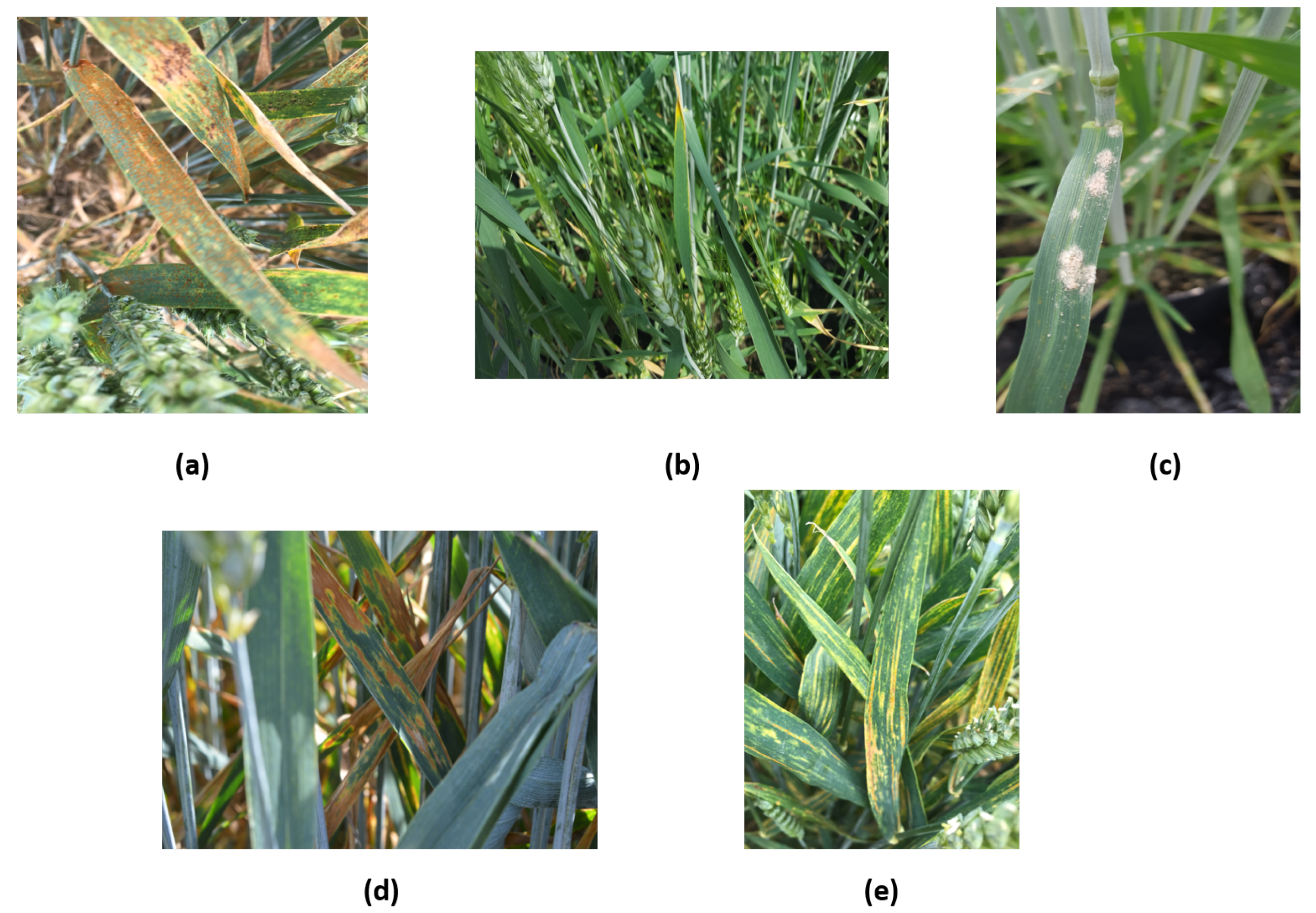
Collecting a high-quality dataset is a crucial step in constructing an effective DL model. In this study, we have collected all the images from two publicly available datasets for wheat disease detection [7,20]. The images were captured between 2019 and 2020 from various locations across the United Kingdom, Ireland, Ethiopia, and Tanzania. All images were labeled by a pathologist. The dataset is composed of 5 classes of wheat, including brown rust, mildew, septoria, yellow rust, and healthy wheat. The images were captured under various lighting conditions, from diverse angles, and against a variety of backgrounds. In addition, deliberate adjustments were made to the distance between the camera and the plant, along with capturing multiple leaves within the image, aimed at introducing variability to the model. This approach differs from typical techniques used in existing works, which primarily rely on publicly available datasets featuring images of zoomed-in plant leaves, often failing to yield accurate results in practical field settings. As shown in Figure 1, the dataset contains a total of 5000 images, which are divided equally into five different classes of wheat crop diseases.
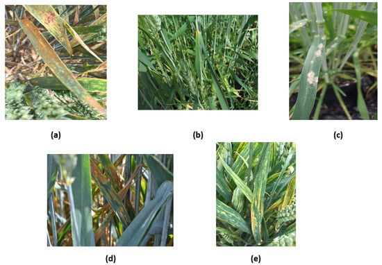
Figure 1.
Sample images from the dataset show difficult field conditions of the five primary wheat conditions: (a) brown rust, (b) healthy, (c) mildew, (d) septoria, and (e) yellow rust.
4.2. Data Preprocessing
To optimize model training and reduce potential flaws during processing, it is imperative to conduct image preprocessing before initiating any data analysis. This is because the accuracy of DL or ML models is largely determined by the quality of the data. As an initial step, the dataset created underwent cleaning to remove any irregularities or corrupted images. Once the dataset was clean, each image was resized to 256 × 256 pixels. This approach helped to avoid the problem of varying image sizes, which could significantly impact the overall performance of the model. We applied the StandardScaler preprocessing function to introduce potential variations in image intensity or color distribution, which can then be normalized, ensuring a more standardized input for the model.
4.3. Data Augmentation
Data augmentation is a method used to expand and diversify a dataset by creating fresh data for training from previous data. This technique is essential for training DL models that rely on a significant amount of data. This technique enhances the model’s capacity to generalize and achieve superior performance on unseen data. Furthermore, it has been demonstrated that using augmentation techniques can effectively minimize overfitting problems [21]. Issues of overfitting may happen during the fine-tuning of CNN models, especially when the initial dataset lacks sufficient images. To mitigate these issues, widely used augmentation methods were employed to expand our training dataset’s size. First, we started by setting a threshold of 1200 images in each class. To balance the proportion of images in each class, we only used augmentation techniques if a class lacked a sufficient number of images set by the threshold. Then, the augmented images were stored in a different location and were only introduced into the training set to avoid overfitting, thereby ensuring the model’s ability to generalize to new data. As detailed in Table 1, every image was randomly rotated between −20° and 20°, with horizontal and vertical shifts ranging from −0.2 to 0.2. Additionally, we performed horizontal flipping, random zooming within the range of 0.8 to 1.2, and brightness and contrast adjustments.

Table 1.
Parameters for data augmentation.
4.4. The Proposed Methodology
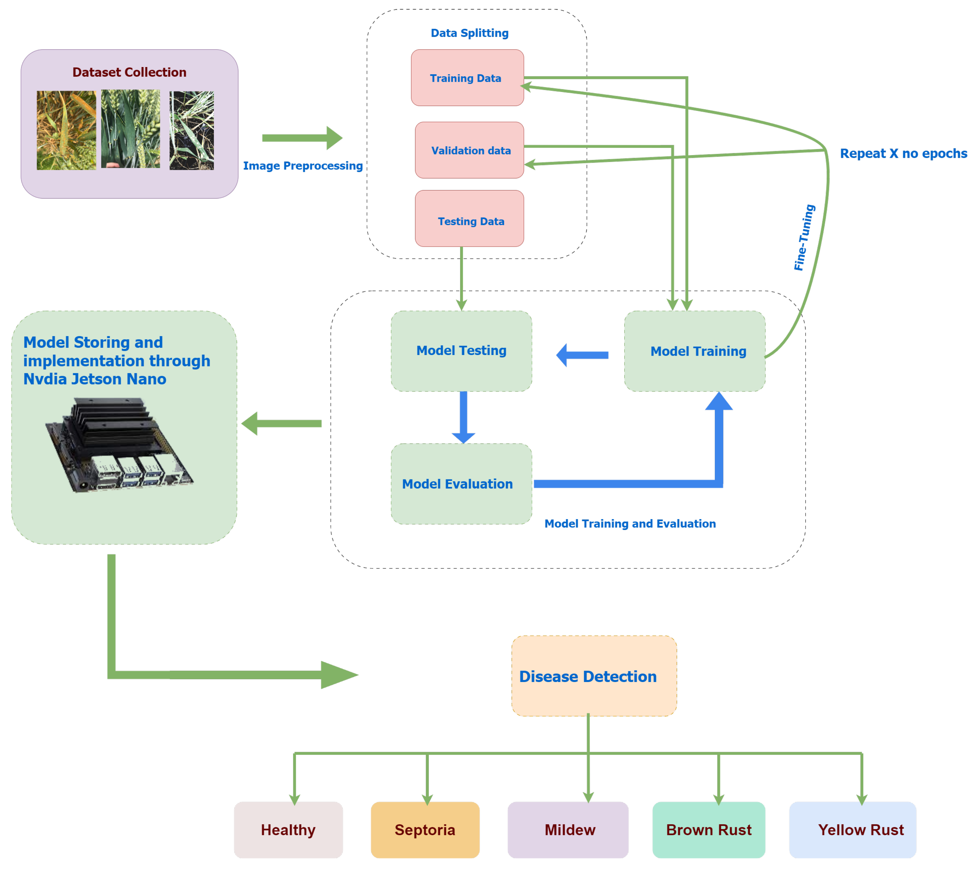
Many studies have been aimed at enhancing the accuracy of plant disease classification by refining and adapting established DL frameworks. In this paper, we deal with feature extraction by freezing the pretrained model and by adding an additional trainable layer that is a custom CNN. Usually, in transfer learning, the dense layers that are trainable are fully connected layers. In this paper, we opt rather to use a trainable CNN and, thus, make the architecture even deeper. We advocate that the pretrained features in transfer learning are more suitable for being fed again to a custom shallow CNN followed by a fully connected layer rather than directly to a fully connected layer. This unique combination of freezing pretrained models and adding custom CNN layers offers a distinctive solution for plant disease classification, diverging from traditional transfer learning methods. Our methodology represents an innovative approach to plant disease classification, combining the power of deep learning with the adaptability of custom CNN layers. This novel approach stands out from conventional transfer learning methods, which typically involve feeding pretrained features directly into fully connected layers. The integration of a custom CNN layer allows for more refined feature extraction and adaptation to the specific requirements of plant disease classification, presenting a promising avenue for enhancing the accuracy of plant disease diagnosis. We have evaluated various deep networks, including CNN and DNN architectures, to use as our custom model. They were trained on a variety of different types of data, including pre-learned features and image data. Pretrained features were taken from ResNet50, EfficientNetB0, EfficientNetB2, MobileNetV2, MobileNetV3Small, DenseNet121, and Inception V3. Figure 2 illustrates the sequential steps of the proposed framework: (a) applying image preprocessing, including normalization and augmentation, (b) splitting the dataset into train, validate, and test, (c) training the models under various situations, such as CNN and DNN, while using pretrained features gathered from ResNet50, EfficientNetB0, EfficientNetB2, MobileNetV2, MobileNetV3Small, DenseNet121, and Inception V3 during the training process, (d) optimizing hyperparameters for optimal training results, (e) analyzing model performance on new unseen data, (f) evaluating overall classification model performance, and (g) storing and loading the optimized model for future use in an embedded system such as Nvidia Jetson Nano to facilitate the ease of use for farmers.

Figure 2.
Diagram illustrating the methodology used in this study.
4.5. Convolutional Neural Network
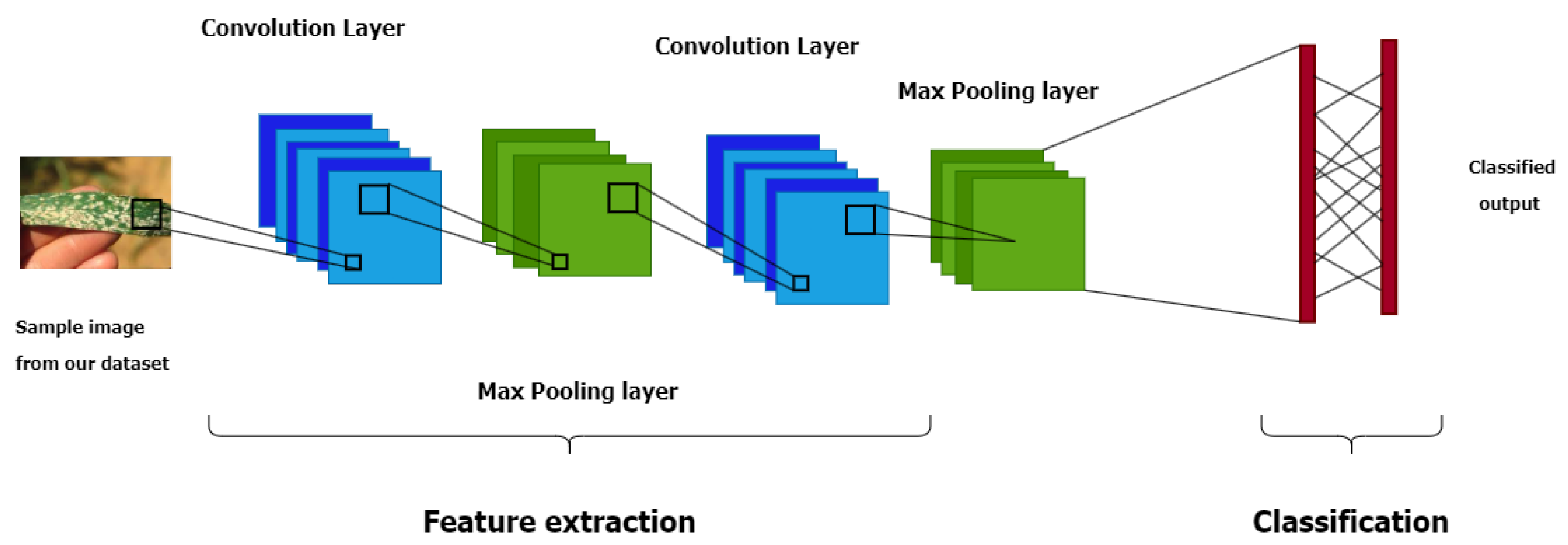
CNN is a well-known DL technique for tasks like object recognition, image classification, and regression. The CNN architecture includes three fundamental layers: an input layer that contains the network’s primary data, hidden layers such as convolutional, max-pooling, and flattened layers, and, finally, a fully connected output layer that receives and flattens inputs from the preceding layers [22]. The structure of CNN is illustrated in Figure 3. CNNs can be utilized in various contexts. Typically, a 1D CNN is employed for sequential data, such as time series or signals. Operating on one-dimensional input data, like a sequence of values along a single axis, it finds applications in tasks like speech recognition, audio analysis, and time series forecasting. On the other hand, 2D CNNs are primarily tailored for image data. Our decision to employ 2D CNNs in our wheat disease detection framework is rooted in several crucial factors. Firstly, 2D CNNs excel in preserving spatial information, making them ideal for image-based tasks where local features play a pivotal role in accurate classification. In the case of wheat leaf images, these local features include subtle discoloration patterns, lesion formations, and other visual cues that are indicative of disease presence. Leveraging 2D CNNs enables us to effectively capture and analyze these features while maintaining the spatial context necessary for precise disease detection. Moreover, the suitability of 2D CNNs for image data simplifies the model architecture, facilitating straightforward processing of input data without the need for complex transformations. Additionally, the core layers of a CNN, such as convolutional and max-pooling layers, are specifically engineered to extract hierarchical features from input images. This enables the model to learn meaningful representations of the data, further enhancing its effectiveness in disease detection.
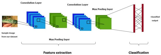
Figure 3.
The strucutre of CNN.
Our approach consists of extra layers like dense layers, dropout layers, and batch normalization. In a CNN, the first layer is in charge of gathering basic features from the input data, including horizontal edges. These features are then fed to the following layers to identify complex features. A CNN’s kernel, padding, and stride size determine how many features exist in each dimension. Convolution is a common method for calculating feature maps in convolutional layers, and it is calculated as defined in Equation (1) [23]:
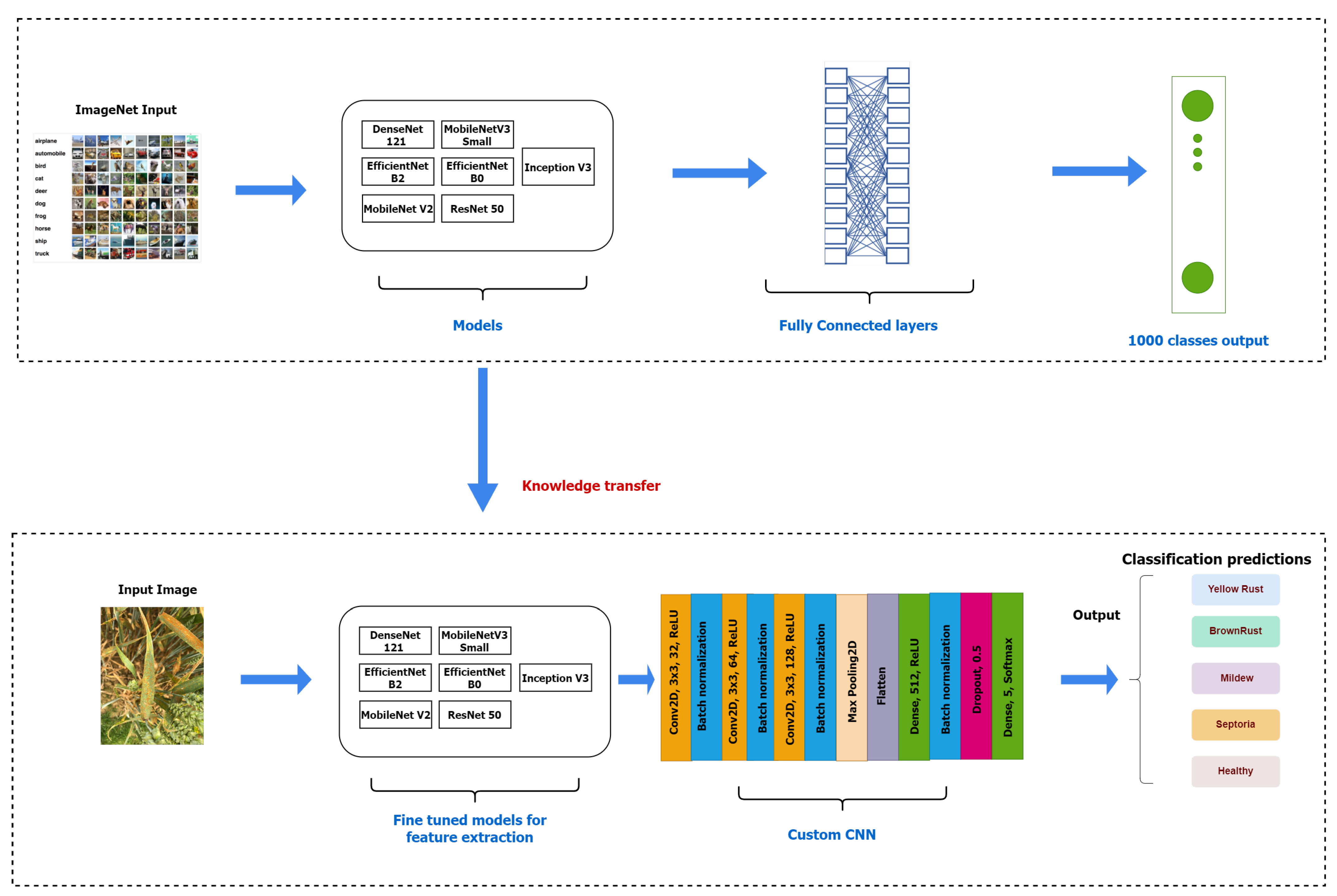
where represents the output feature map, is the input feature map, denotes the convolutional filter weights, and is the bias term. The pooling layer minimizes the spatial dimensions of the convoluted feature, requiring fewer computational requirements for data processing. In this work, we have used max-pooling. In fact, max-pooling selects the maximum pixel value within the kernel or filter’s coverage area. Using a max-pooling layer of size (2, 2) for the regained matrix resolved the overfitting issue. Dense layers are utilized to recognize images according to the output generated by the convolutional layers. Dropout layers avoid overfitting by deactivating connections between hidden units (neurons) and setting them to zero during training updates. We used a dropout of 0.5. Flattening is the process of converting data into a 1D array that can be passed to subsequent layers. In this study, we implemented a custom CNN network to evaluate classification performance. Our focus was on creating a model that is simple yet effective, lightweight, and suitable for implementation on resource-limited devices in real-world scenarios. The model architecture comprised three convolutional layers with 32, 64, and 128 filters, all utilizing a kernel size of 3 × 3; the input was 256 × 256 × 3, i.e., the image dimensions. Each convolutional layer was followed by batch normalization to ensure stable training. After the last convolutional layer, we added a max-pooling layer with a size of 2 × 2. Finally, we flattened the output of the CNN layers and passed it to a fully connected layer with 512 neurons, followed by batch normalization and a dropout rate of 0.5. This technique helps remove overfitting by introducing a form of regularization. The final fully connected layers acted as classifiers using the softmax function. They consisted of 5 units, corresponding to the class count of the model. As shown in Figure 4, the CNN structure consists of two different models that use various TL techniques to train image data in order to detect wheat leaf diseases.
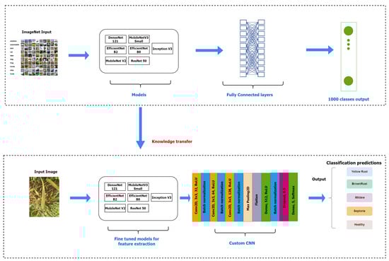
Figure 4.
Integration of the custom CNN with transfer learning networks.
CropNet
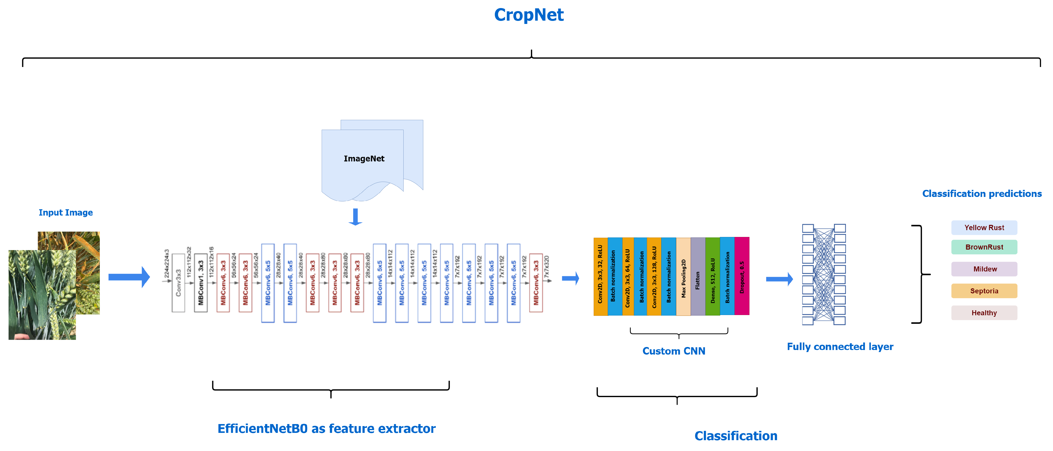
In the new hybrid approach, CropNet, EfficientNetB0 is paired with a Custom CNN model consisting of three Conv2D layers with 32, 64, and 128 filters, each with a kernel size of 3 × 3, followed by batch normalization. Additionally, a max-pooling layer with a size of 2 × 2 is incorporated. The top input layer of the EfficientNetB0 is frozen and defined as non-trainable. Then, the custom model is added, followed by a ReLU layer with 512 neurons, batch normalization, and a dropout layer with a rate of 0.5 to avoid overfitting and to enhance model generalization. Finally, a fully connected layer with a softmax function is incorporated as the final layer to classify the five wheat diseases. An illustration of CropNet architecture is presented in Figure 5.
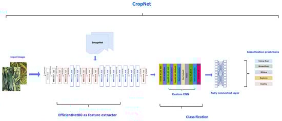
Figure 5.
Architecture of our proposed model CropNet.
4.6. Deep Neural Networks
A DNN is a neural network with many hidden layers and numerous neurons that perform basic computations. The DNN model is known for its robust and basic DL structure [24]. A DNN model is split into three categories: input, hidden, and output. The classification method’s input layer incorporates all features from the constructed feature space. Six implicit layers are used to predict the classified image. After several experiments, the model was constructed with six hidden layers, each with 512, 256, 256, 64, 64, and 32 neurons, arranged sequentially. Each hidden layer is made up of a dense layer with ReLU as the activation function, a batch normalization layer that normalizes the activations of the previous layer at each batch, thereby stabilizing and accelerating the learning process, and a dropout layer with 0.5 as a rate value that randomly drops a proportion of neurons during training to prevent overfitting. The model was trained with 30 batches using the Adamax optimizer over 100 epochs. Figure 4 shows the building of the DNN model, which uses image data based on TL. The extracted features were joined to create a new attribute for identifying a specific class among five diseases.
4.7. Hyperparameter Tuning
The process of learning in any DL models depends on the values of hyperparameters during the training phase. For the improved CropNet model and all the models we tested, we carefully adjusted the hyperparameters to improve accuracy and performance. After testing different optimizers, such as Adam, Adamax, and Adadelta, we found that Adamax significantly improved CropNet performance [25]. Its adaptive learning rates and combination of AdaGrad and RMSProp benefits enhanced convergence and training efficiency. Additionally, utilizing the ReLU activation function further boosted performance by addressing the vanishing gradient problem and accelerating convergence, resulting in higher accuracy and faster convergence when combined with Adamax. The model was trained for 100 epochs. For training purposes, the initial learning rate was reduced to gradually increase accuracy. At first, we fixed the learning rate to 1 × 10 and then adjusted it after each epoch using the ReduceLearningRateOnPlateau method from Keras [26]. We reduced the learning rate using a factor of 0.5 based on the monitored training accuracy, with a set patience parameter using Equation (2):
After every epoch, the learning rate (LR) was reduced by half if the training accuracy dropped. The ReduceLearningRateOnPlateau(RLR-ONPlateau) approach switched to monitoring the validation loss and adjusted the LR as needed once the training accuracy reached a threshold of 0.9. We used an early stopping technique, setting the patience threshold to 3 epochs. This technique helps prevent overfitting, ensuring that the model generalizes well to new, unseen data, and prevents unnecessary computation and time spent on training. This enables us to stop the training process if the monitored value does not improve after three epochs. As a loss function, we used the categorical cross-entropy, which combines a cross-entropy loss with a softmax max activation. The categorical cross-entropy loss function is well-suited for multi-class classification tasks like the detection of wheat leaf diseases [27]. The following equation (Equation (3)) defines the categorical cross-entropy.:
A list of hyperparameters is shown in Table 2.
Table 2.
Hyperparameters for all CNN models.
4.8. Model Training
In total, we divided 5000 non-augmented and 1000 augmented images into three categories. First, 80% were designated for training, which amounted to 4000 non-augmented and 1000 augmented samples. We only included the augmented data in the training set. Additionally, 10% of the data (500 samples) were allocated to the validation set, and the remaining 10% (500 samples) were reserved for testing. The model utilizes the training data to recognize patterns and enhance accuracy. During the training process, the validation data isare employed to validate the model’s performance. This validation data are fed to the model in batches, serving as a form of testing at each step of training. After that, we used the test data, which included samples that were unseen by the model, to analyze the model’s efficiency. This offers an overview of the model’s accuracy on new, unseen data. The models underwent training and testing on an HP ProLiant ML350 Gen10 server featuring 64 Intel Xeon CPU Gold 5218 processors, each operating at 2.30 GHz. With a substantial 256 GB of RAM, the server ran on the Windows Server 2016 Datacenter 64-bit operating system. Python 3 served as the primary programming language for model implementation, complemented by essential libraries, including Keras, OpenCV, and Matplotlib, which are essential in both the development and comparison phases of the models.
4.9. Model Selection
The best model among the pretrained network-based CNN, custom CNN, or pretrained network-based DNN models needed to be selected in this phase. We were able to evaluate the efficiency of each model after training and testing them. Certain models outperformed others. Therefore, we could evaluate the capabilities of the models and select the top-performing DL model.
4.10. Performance Evaluation Metrics
In this study, quantitative analysis was utilized to assess classification performance. Evaluation metrics such as precision, recall, overall accuracy, and F1-Score were employed for comparing and analyzing classification performance. Any ML or DL model’s classification results usually include four cases: T and F, which represent the true or false status of the model’s prediction, or P and N, which denote a positive or negative class, respectively. The model’s performance can be evaluated by calculating the ratio between the different prediction outcomes.
4.11. Proposed IoT System for Wheat Disease Detection
After selecting the best lightweight model, it can be implemented on an embedded device within a system that utilizes an IoT-based wireless network of cameras for gathering field images. Subsequently, these collected images are transmitted to an edge device for real-time disease diagnosis in the field. A camera captures real-time data and sends them to the device. Given the model’s minimal parameters and compact size, any edge device could be used, but we suggest the Nvidia Jetson Nano due to its affordability and popularity within the edge device community [28,29,30]. The edge device would then identify the disease affecting the leaf and alert the user—in this case, the farmer—using a mobile application via various IoT communication protocols, potentially integrated with smart spray technology. This approach ensures both both prompt and precise diagnosis of wheat crop diseases while minimizing latency, as all processing occurs locally without requiring intervention from farmers.
5. Results and Discussion
Performance evaluation in deep learning image classification typically involves tracking training loss and accuracy. Training accuracy refers to the model’s ability to produce precise predictions based on training data. On the other hand, the training loss is calculated based on the percentage of errors made by the model in predicting the training data, which can be easily reduced by tuning the model parameters. In this study, we have constructed various DL models and evaluated different architectures to detect wheat leaf diseases, focusing on lightweight models with few parameters and size. We combined our custom CNN and DNN with pretrained models to serve as feature extractors. We compared their accuracies and losses to choose a model that was suitable for our task; the results are discussed in the following sections. The models were trained using the same collected dataset and parameters in order to ensure an even evaluation. We tested with and without data augmentation, and we were able to confirm that data augmentation enhances the performance of all the proposed models [31].
5.1. Custom DNN with Pretrained Feature Extractors
To enhance wheat disease detection, we evaluated the effectiveness of DNNs when combined with transfer learning approaches for feature extraction. Data augmentation techniques were employed to expand the dataset. Eight different pretrained CNN models were trained, validated, and tested; their performance results are presented in Table 3 and Table 4. Based on the results, the combination of custom DNN with EfficientNetB0 achieved the highest performance among all the models tested in this study, with an accuracy of 95.20% and precision, recall, and F1-score all having the same value.
Table 3.
The expected outcomes of DNN models using various fine-tuned deep network models.
Table 4.
The performance of the DNN algorithms on the testing set.
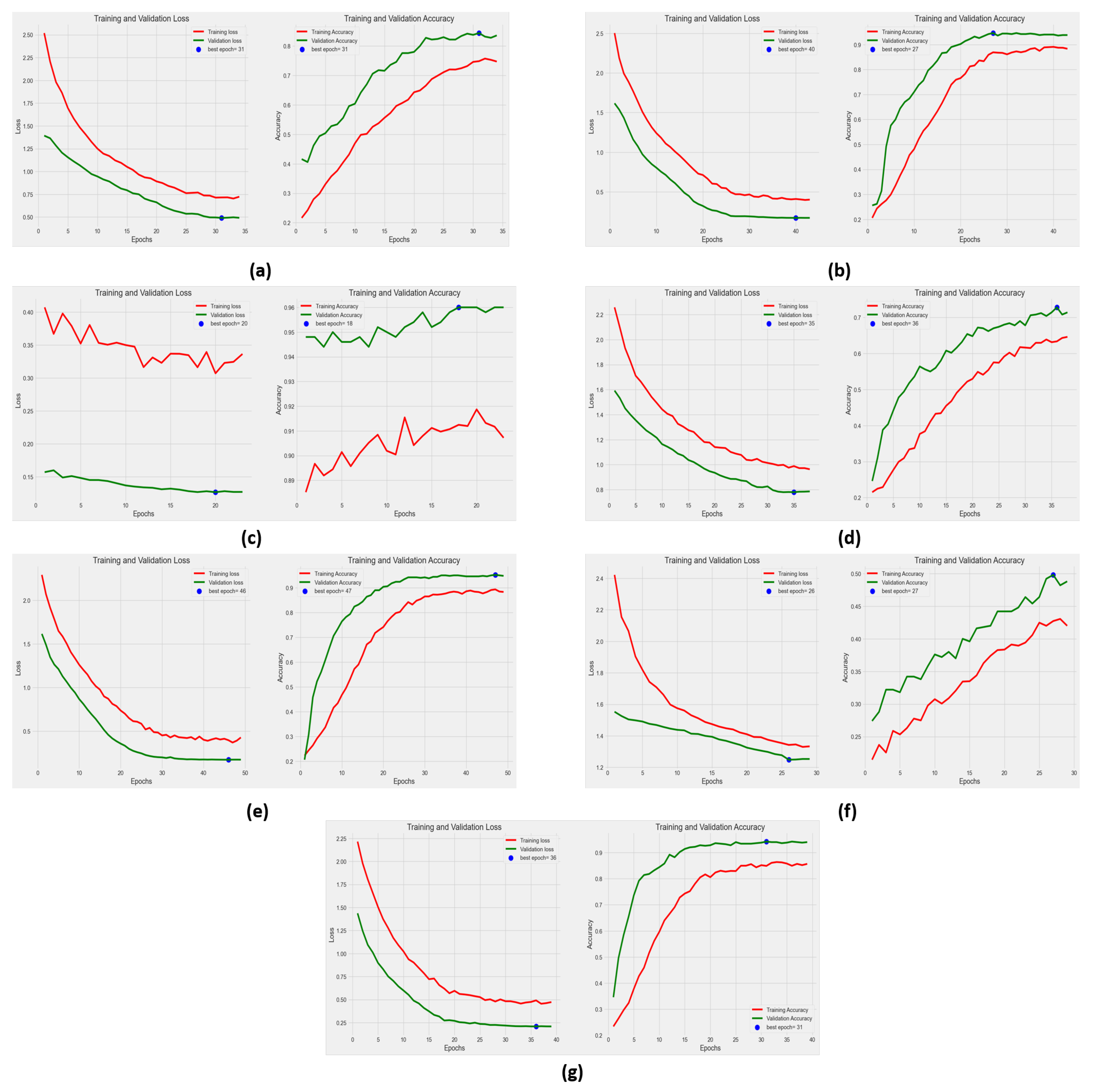
The above model demonstrated validation and training accuracies of 96% and 95.20%, respectively, along with validation and training losses of 0.127 and 0.307. Based on these values, we can suggest that the model is capable of generalizing to new data, as it performed well not only on the training set but also on the validation set. However, all the other models outperformed DNN+InceptionV3. The model exhibited very low performance, with a testing accuracy of 43%, alongside 41%, 48%, 1.33, and 0.25 as training accuracy, validation accuracy, training loss, and validation loss, respectively. This can be due the the fact that InceptionV3 has a more complex architecture, which can make it difficult to modify and fine-tune with another custom model. DNN+MobileNetV3Small outperformed MobileNetV2, with an increase in testing, training, and validation accuracy of almost 20%, consistent with Howard et al. [32], who confirmed that MobileNetV3 is both more accurate and faster than MobileNetV2. Figure 6 shows the learning curves of the DNN models with augmented data, The DNN+MobileNetV3-Small, DNN+EfficientNetB2, and DNN+ResNet50 models exhibited reliable validation accuracies of 95% (with a loss of 0.171), 93.8% (with a loss of 0.171), and 94% (with a loss of 0.208), respectively. The learning curves for these models showed a favorable convergence rate, with steady decreases in loss and gradual improvements in training and validation accuracy over epochs. The DNN+EfficientNetB0 model, on the other hand, shows an unusual curve with great validation accuracy and loss rates of 96% and 0.127. While the validation curve shows a slight improvement over epochs, the training loss remains constant throughout, suggesting that the model has reached its learning capacity. This indicates the necessity for fine-tuning, hyperparameter adjustments, or architectural improvements.
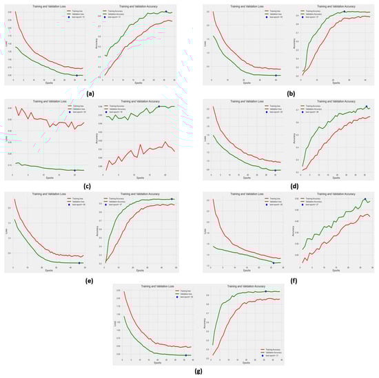
Figure 6.
Evaluation measures for various DNN networks: (a) DenseNet121+DNN, (b) EfficientNetB2+DNN, (c) EfficientNetB0+DNN, (d) MobileNetV2+DNN, (e) MobileNetV3Small+DNN, (f) InceptionV3+DNN, (g) ResNet50+DNN.
The aforementioned results align with the research conducted by Reddy et al. [33], which demonstrated DNNs’ exceptional ability to identify and detect plant leaf diseases. This highlights DNNs’ important role in the horticulture industry.
5.2. Custom CNN with Pretrained Feature Extractors
We evaluated the CNNs’ efficiency in detecting various types of wheat diseases that are difficult to identify with the naked eye. We employed transfer learning, such as EfficientNetB0 and B2, InceptionV3, MobileNetV3Small, MobileNetV2, ResNet50, and DenseNet121, to improve performance while reducing training time and computational costs. Data augmentation was used to expand and diversify the dataset. For each network, once the features had been collected, they were used to train a custom CNN. The training of these models was set to stop after 3 consecutive epochs without improvement in the monitored value. Therefore, each model required a different number of epochs to converge. The validation, training accuracy, and loss across the models are presented in Table 5, while the overall performances, including the test accuracy, precision, recall, and F1-score, can be viewed in Table 6. The custom CNN model reached a validation accuracy of 84% and a testing accuracy of 86.40%.
Table 5.
The predicted results of the CNN-based models using various fine-tuned deep network models.
Table 6.
The performance of the CNN algorithms on the testing set.
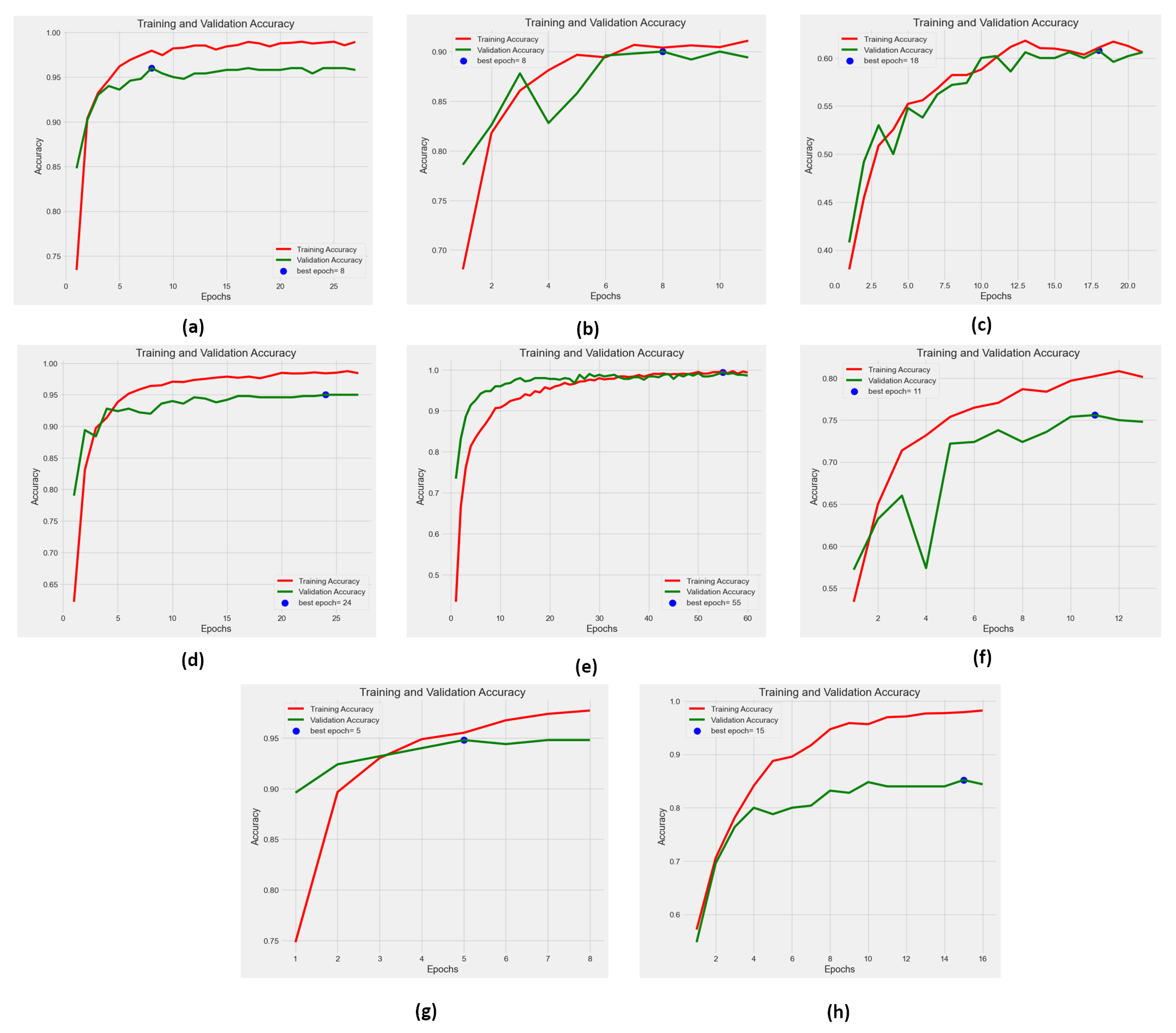
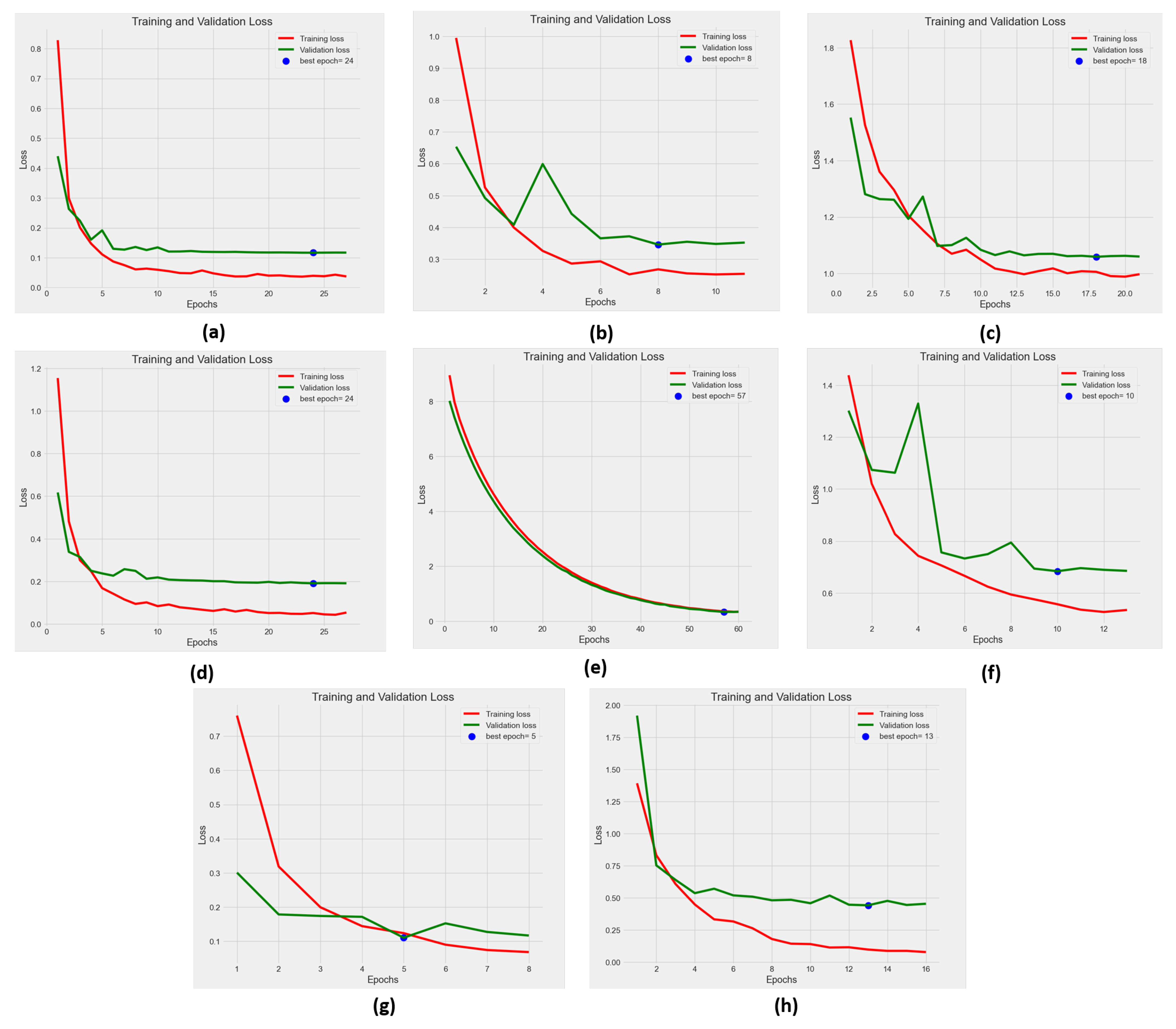
The model performed significantly well, but there is a noticeable variance between the training accuracy of 98% and the validation accuracy of 84%, indicating that the model may be overfitting. This is further supported by the large gap shown in Figure 7 between the training and validation accuracy curves. To enhance the outcomes of our designed model and ensure accurate predictions with exceptional results, we integrated pretrained networks to extract additional features. The behavior of the models was closely monitored by calculating the accuracy and losses at every epoch during both the training and validation phases, as shown in Figure 7 and Figure 8.
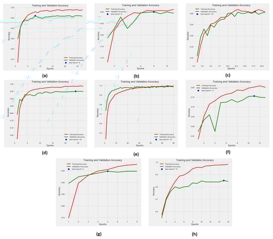
Figure 7.
Evaluation of the accuracy measures for various CNN networks: (a) ResNet50+CustomCNN, (b) DenseNet121+CustomCNN, (c) InceptionV3+CustomCNN, (d) MobileNetV3Small+CustomCNN, (e) CropNet, (f) MobileNetV2+CustomCNN, (g) EfficientNetB2+CustomCNN, (h) CustomCNN.
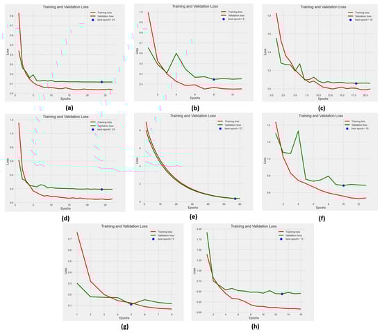
Figure 8.
Evaluation of the loss measures for various CNN networks: (a) ResNet50+CustomCNN, (b) DenseNet121+CustomCNN, (c) InceptionV3+CustomCNN, (d) MobileNetV3Small+CustomCNN, (e) CropNet, (f) MobileNetV2+CustomCNN, (g) EfficientNetB2+CustomCNN, (h) CustomCNN.
Using DenseNet121 improved the accuracy of the custom CNN model by 2% and reduced the validation loss by 0.2. However, combining CNN with InceptionV3 resulted in a significant loss in accuracy, decreasing by 27%. This combination was not successful, likely due to InceptionV3’s complex architecture, which can make it challenging to modify and fine-tune with another custom model. Moreover, the combination of CNN with ResNet50, MobileNetV3-Small, and EfficientNetB2 remarkably enhanced the results of the deep network. They reached outstanding results in all metrics, with overall accuracies of 95%, 92%, and 98%, respectively.
Based on these outcomes, we can conclude that EfficientNet surpassed other algorithms. EfficientNetB0, in particular, is regarded as both simple and effective in plant disease classification due to its remarkable ability to achieve high accuracy rates with minimal complexity. Despite its simplicity, EfficientNetB0 excels in plant disease classification tasks because its architecture allows it to effectively learn and represent complex patterns within the data [34]. In this study, EfficientNetB0 is the selected method for our feature extraction process.
CropNet Performances
CropNet achieved outstanding results, surpassing all other models across all metrics, with an accuracy rate of 99.80%, a train accuracy of 99%, and a loss of 0.3. Precision, recall, and F1-score were all approximately 100%. Powered by data augmentation, the CropNet hybrid network has proven to be a successful model for evaluating plant health. Its outstanding architecture enabled it to surpass all previous techniques and establish a new standard for wheat leaf diagnostics.
Figure 7e and Figure 8e shows that CropNet began converging at lower epochs, indicating a more suitable balance between model fitting and complexity. Both validation and training accuracies continued to gradually improve until the model achieved full convergence, having a remarkable a validation accuracy of 99% and a loss of 0.29, surpassing all other models. The training accuracy and loss closely align with the values of the validation accuracy and loss. As the accuracy increases, the loss decreases and they both stabilize, making a model that is less susceptible to overfitting compared to others, resulting in an optimal fit. In addition, from the curves illustrated below, we conclude that the models using ResNet50, MobileNet3Small, and EfficientNetB2 demonstrated good behavior, as they converged very quickly and reached full convergence at epochs 10, 25, and 5, respectively. They exhibited a steady decrease in the loss values of both training and validation sets, although not as good as the metrics seen with CropNet. We have incorporated an early stopping mechanism to prevent overtraining, where each model stops training after three consecutive epochs without improvement in the monitored metric.
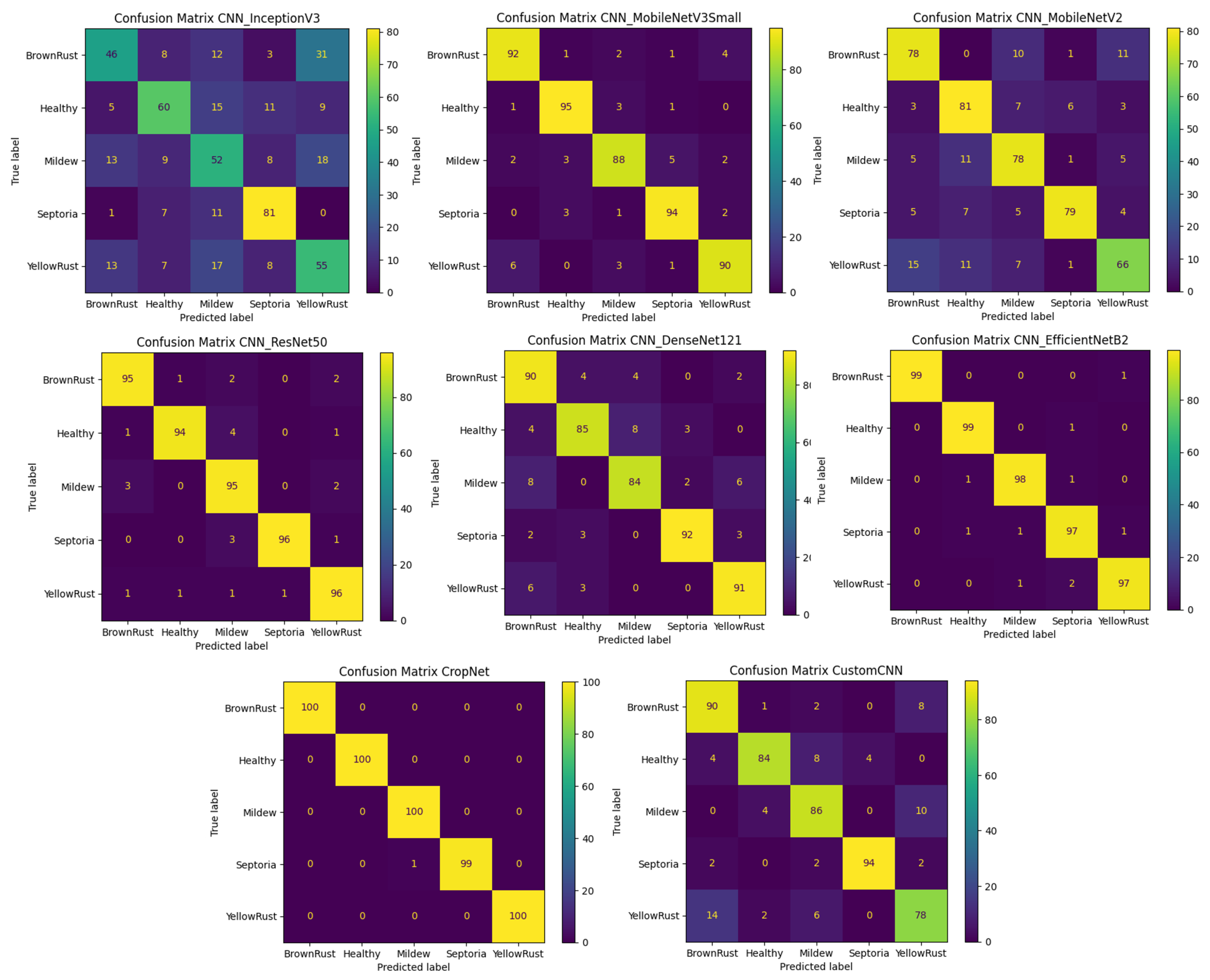
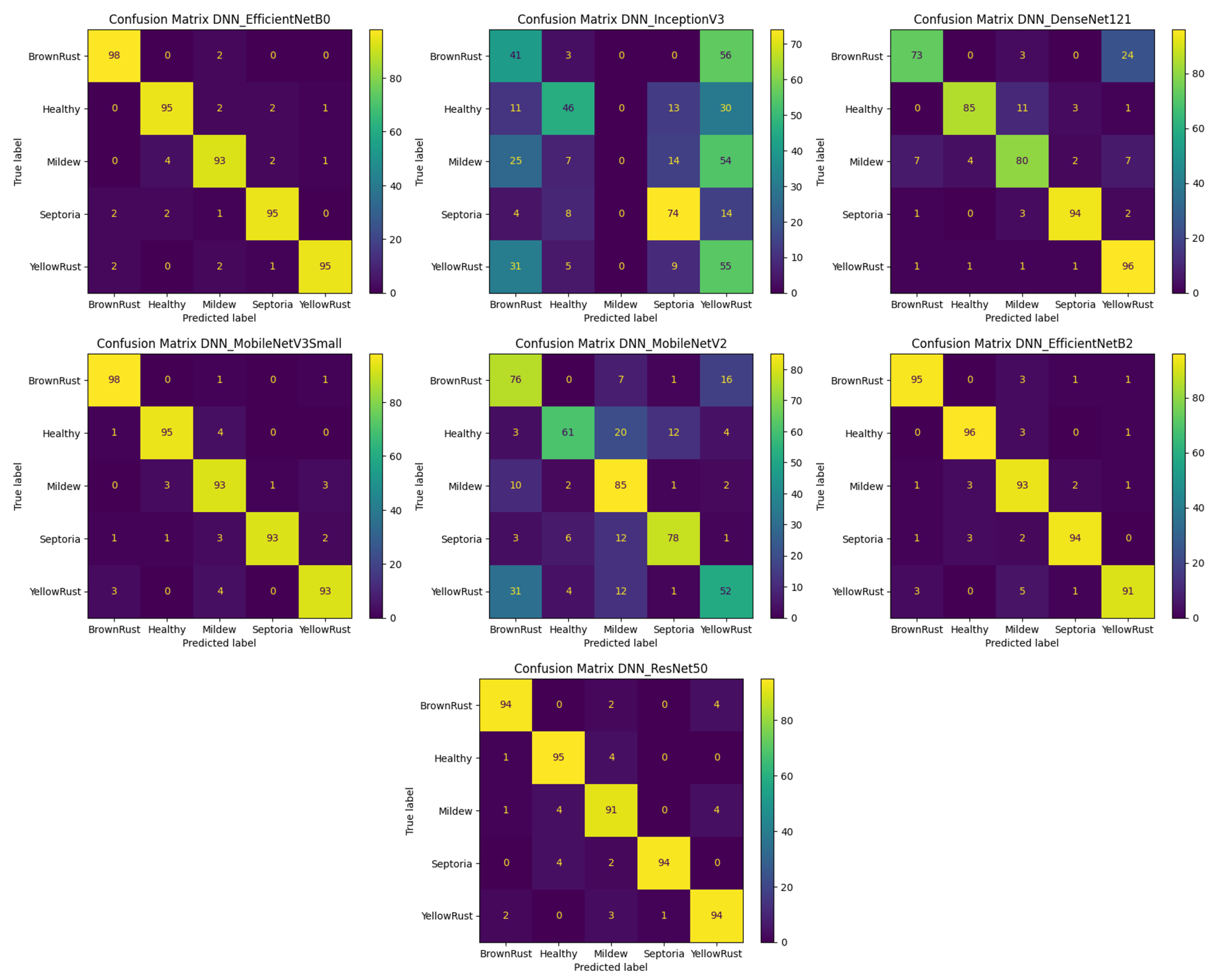
5.3. Confusion Matrix Analysis
A popular metric in image classification is the confusion matrix, which allows us to distinguish accurately and inaccurately classified images across various classes in order to assess a model’s performance [35]. The actual class instances are represented by each column of the matrix, while the predicted class instances are represented by each row. The proposed CNN and DNN combined with transfer learning approach models for wheat disease detection are shown via a confusion matrix in Figure 9 and Figure 10 during the testing phase. In a testing dataset containing 500 images, an analysis showed that CNN+InceptionV3, DNN+InceptionV3, CNN+MobileNetV3-Small, CNN+MobileNetV2, and DNN+MobileNetV2 misclassified roughly 206, 284, 41, 118, and 148 images, respectively. The CNN+ResNet50 model had only 2 instances of false negatives (FNs), where the model misclassified wheat leaves as healthy despite being affected by a disease. When this rate is high, it can present a severe threat to the crop, particularly if the disease is viral and can spread quickly across the field. On the other hand, CropNet presented exceptional results, as it outperformed the other models. It exhibited zero false negatives and zero false positives, with only one misclassified instance due to the similarity in patterns between the two classes. Because of to its remarkable efficacy in comparison to previous research, our improved CropNet model is a good fit for analyzing wheat leaf health.
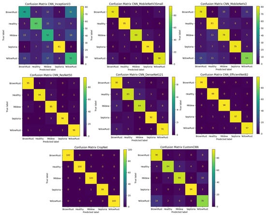
Figure 9.
Confusion matrixes for the CNNs.
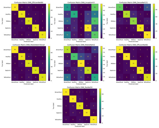
Figure 10.
Confusion matrixes for the DNNs.
6. Further Discussion
We noticed that most research conducted in this field often relies on one or two architectures to detect a single disease. However, it is crucial to compare several architectures to determine the most suitable one with the highest accuracy and lower complexity. In this research, we present CropNet, a lightweight model for wheat leaf disease detection using hybrid deep networks based on RGB images. Our work differs from previous studies in that we conducted a thorough comparison of multiple deep network algorithms to identify various diseases on wheat crops. We developed a lightweight model with a size of only 51 MB, containing 6 million parameters, and achieved a superior accuracy of 99.80%, while minimizing both model complexity and computational requirements. CropNet’s impressive performance renders it a promising tool for practical applications in smart agriculture. Table 7 illustrates that CropNet’s compact size makes it appropriate to be used with IoT microprocessors. Table 7 shows the total number of parameters, including both trainable and non-trainable parameters. The overall number of parameters indicates the number of calculations that each model must perform at each timestamp.
Table 7.
Comparison of model efficiency.
To create the CropNet model, we employed a transfer learning approach, coupling EfficientNetB0 with a shallow CNN specifically developed for this study. Combining EfficientNetB0 and CNN in a single model can generate a network that is ideal for image recognition applications. EfficientNetB0 is a pretrained DL model. Using EfficientNetB0 for feature extraction enables one to find patterns and features that traditional machine learning algorithms can overlook. The custom CNN utilized in the hybrid approach has the capacity to acquire various levels of abstract representations from the collected features. This capability aids in capturing nuanced and complex relationships within the data. Training a model from zero is time-consuming and requires substantial resources. Utilizing transfer learning techniques, as in this hybrid approach, reduces time and costs while enhancing model generalization. To further test the efficiency of the new proposed CropNet model, we compared our results with several studies (Table 8). We evaluated the methods used, the types of crops, and their results. Based on these results, we can conclude that our study presented a thorough and comprehensive comparison of multiple techniques and different methods to produce CropNet. This model surpasses existing research in terms of model size and number of parameters, and provides a superior classification score, which makes it a good candidate to be embedded in resource-constrained environments, such as for farmers in real-life situations.
Table 8.
Comparative analysis of recently published works.
7. Conclusions and Future Work
A crop of global importance like wheat is frequently affected by numerous diseases. To reduce production losses and contain the spread of these diseases, we require not just accurate but also timely diagnosis. Deep learning advancements have created new avenues and opportunities for precise and effective plant disease detection. In this research, we conducted an extensive comparison using various architectures to introduce an innovative hybrid approach named CropNet. This model has shown promising results in terms of classification accuracy, and it has a compact size with few parameters. It is important to note that, while the CropNet model has demonstrated promising results in identifying diseases as well as healthy leaves in wheat, its accuracy might decrease, especially when differentiating between closely related diseases. Furthermore, its performance could be constrained by the model’s inability to distinguish between specific diseases. In addition, it is worth noting that the dataset utilized in this study may not comprehensively represent the diverse range of disease presentations that can manifest in wheat. This limitation could potentially restrict the applicability of the model to real-world scenarios. Our proposed hybrid deep learning model achieves an accuracy of 99.80% in classifying four diseases of wheat leaves and healthy leaves, even on a small dataset. CropNet will be integrated into an IoT-based framework alongside an object detection model that is responsible for identifying wheat leaves. Subsequently, CropNet will detect diseases in the wheat leaves. Once a disease is detected, the system will automatically recommend the appropriate spray treatment for the identified disease. To further enhance the capabilities and applicability of CropNet, future research directions could include testing the model on other crops or diseases to enhance its generalizability and adaptability. Moreover, CropNet can also be improved to perform well in diverse environmental conditions such as varying weather patterns, soil types, and climate zones. This could involve incorporating additional data modalities, such as weather data or soil composition. Additionally, CropNet can be seamlessly integrated with other agricultural technologies such as precision agriculture or precision irrigation, to enhance overall agricultural productivity and sustainability.
Author Contributions
Conceptualization, O.J., M.O.-E.A., K.S. and A.Y.; methodology, O.J., M.O.-E.A., K.S. and A.Y.; software, O.J., M.O.-E.A., K.S. and A.Y.; validation, O.J., M.O.-E.A., K.S. and A.Y.; formal analysis, O.J., M.O.-E.A., K.S. and A.Y.; investigation, O.J., M.O.-E.A., K.S. and A.Y.; resources, O.J., M.O.-E.A., K.S. and A.Y.; data curation, O.J., M.O.-E.A., K.S. and A.Y.; writing—original draft preparation, O.J., M.O.-E.A., K.S. and A.Y.; writing—review and editing, O.J., M.O.-E.A., K.S. and A.Y.; visualization, O.J., M.O.-E.A., K.S.,and A.Y.; supervision, O.J., M.O.-E.A., K.S. and A.Y.; project administration, O.J., M.O.-E.A., K.S. and A.Y. All authors have read and agreed to the published version of the manuscript.
Funding
This research received no external funding.
Institutional Review Board Statement
Not applicable.
Informed Consent Statement
Not applicable.
Data Availability Statement
Dataset available on request from the authors.
Conflicts of Interest
The authors declare no conflicts of interest.
References
- Erenstein, O.; Jaleta, M.; Mottaleb, K.A.; Sonder, K.; Donovan, J.; Braun, H.J. Global trends in wheat production, consumption and trade. In Wheat Improvement: Food Security in a Changing Climate; Springer International Publishing: Cham, Switzerland, 2022; pp. 47–66. [Google Scholar]
- Bhola, A.; Kumar, P. Deep feature-support vector machine based hybrid model for multi-crop leaf disease identification in Corn, Rice, and Wheat. Multimed. Tools Appl. 2024, 1–21. [Google Scholar] [CrossRef]
- Pantazi, X.E.; Moshou, D.; Tamouridou, A.A. Automated leaf disease detection in different crop species through image features analysis and One Class Classifiers. Comput. Electron. Agric. 2019, 156, 96–104. [Google Scholar] [CrossRef]
- Huang, L.; Liu, Y.; Huang, W.; Dong, Y.; Ma, H.; Wu, K.; Guo, A. Combining random forest and XGBoost methods in detecting early and mid-term winter wheat stripe rust using canopy level hyperspectral measurements. Agriculture 2022, 12, 74. [Google Scholar] [CrossRef]
- Waldamichael, F.G.; Debelee, T.G.; Schwenker, F.; Ayano, Y.M.; Kebede, S.R. Machine learning in cereal crops disease detection: A review. Algorithms 2022, 15, 75. [Google Scholar] [CrossRef]
- Prodeep, A.R.; Hoque, A.M.; Kabir, M.M.; Rahman, M.S.; Mridha, M. Plant disease identification from leaf images using deep CNN’S efficientnet. In Proceedings of the 2022 International Conference on Decision Aid Sciences and Applications (DASA), Chiangrai, Thailand, 23–25 March 2022; pp. 523–527. [Google Scholar]
- Jouini, O.; Sethom, K.; Bouallegue, R. Wheat leaf disease detection using CNN in Smart Agriculture. In Proceedings of the 2023 International Wireless Communications and Mobile Computing (IWCMC), Marrakesh, Morocco, 19–23 June 2023; pp. 1660–1665. [Google Scholar]
- Elsherbiny, O.; Elaraby, A.; Alahmadi, M.; Hamdan, M.; Gao, J. Rapid Grapevine Health Diagnosis Based on Digital Imaging and Deep Learning. Plants 2024, 13, 135. [Google Scholar] [CrossRef]
- Ghosh, P.; Mondal, A.K.; Chatterjee, S.; Masud, M.; Meshref, H.; Bairagi, A.K. Recognition of sunflower diseases using hybrid deep learning and its explainability with AI. Mathematics 2023, 11, 2241. [Google Scholar] [CrossRef]
- Orchi, H.; Sadik, M.; Khaldoun, M.; Sabir, E. Automation of crop disease detection through conventional machine learning and deep transfer learning approaches. Agriculture 2023, 13, 352. [Google Scholar] [CrossRef]
- Tang, Z.; Yang, J.; Li, Z.; Qi, F. Grape disease image classification based on lightweight convolution neural networks and channelwise attention. Comput. Electron. Agric. 2020, 178, 105735. [Google Scholar] [CrossRef]
- Verma, S.; Kumar, P.; Singh, J.P. A unified lightweight CNN-based model for disease detection and identification in corn, rice, and wheat. IETE J. Res. 2023, 1–12. [Google Scholar] [CrossRef]
- Aboneh, T.; Rorissa, A.; Srinivasagan, R.; Gemechu, A. Computer vision framework for wheat disease identification and classification using Jetson GPU infrastructure. Technologies 2021, 9, 47. [Google Scholar] [CrossRef]
- Hamzaoui, M.; Ould-Elhassen Aoueileyine, M.; Romdhani, L.; Bouallegue, R. An Improved Deep Learning Model for Underwater Species Recognition in Aquaculture. Fishes 2023, 8, 514. [Google Scholar] [CrossRef]
- Hayajneh, A.M.; Aldalahmeh, S.A.; Alasali, F.; Al-Obiedollah, H.; Zaidi, S.A.; McLernon, D. Tiny machine learning on the edge: A framework for transfer learning empowered unmanned aerial vehicle assisted smart farming. IET Smart Cities 2024, 6, 10–26. [Google Scholar] [CrossRef]
- Shafik, W.; Tufail, A.; De Silva Liyanage, C.; Apong, R.A.A.H.M. Using transfer learning-based plant disease classification and detection for sustainable agriculture. BMC Plant Biol. 2024, 24, 136. [Google Scholar] [CrossRef] [PubMed]
- Račič, M.; Oštir, K.; Zupanc, A.; Čehovin Zajc, L. Multi-Year Time Series Transfer Learning: Application of Early Crop Classification. Remote Sens. 2024, 16, 270. [Google Scholar] [CrossRef]
- Zhao, Y.; Han, S.; Meng, Y.; Feng, H.; Li, Z.; Chen, J.; Song, X.; Zhu, Y.; Yang, G. Transfer-learning-based approach for yield prediction of winter wheat from planet data and SAFY Model. Remote Sens. 2022, 14, 5474. [Google Scholar] [CrossRef]
- Al Sahili, Z.; Awad, M. The power of transfer learning in agricultural applications: AgriNet. Front. Plant Sci. 2022, 13, 992700. [Google Scholar] [CrossRef] [PubMed]
- Long, M.; Hartley, M.; Morris, R.J.; Brown, J.K. Classification of wheat diseases using deep learning networks with field and glasshouse images. Plant Pathol. 2023, 72, 536–547. [Google Scholar] [CrossRef] [PubMed]
- Shorten, C.; Khoshgoftaar, T.M. A survey on image data augmentation for deep learning. J. Big Data 2019, 6, 1–48. [Google Scholar]
- Jouini, O.; Sethom, K.; Bouallegue, R. The Impact of the Application of Deep Learning Techniques with IoT in Smart Agriculture. In Proceedings of the 2023 International Wireless Communications and Mobile Computing (IWCMC), Marrakesh, Morocco, 19–23 June 2023; pp. 977–982. [Google Scholar]
- Krizhevsky, A.; Sutskever, I.; Hinton, G.E. ImageNet classification with deep convolutional neural networks. Commun. ACM 2017, 60, 84–90. [Google Scholar] [CrossRef]
- Schmidhuber, J. Deep learning in neural networks: An overview. Neural Networks 2015, 61, 85–117. [Google Scholar] [CrossRef]
- Saleem, M.H.; Potgieter, J.; Arif, K.M. Plant disease classification: A comparative evaluation of convolutional neural networks and deep learning optimizers. Plants 2020, 9, 1319. [Google Scholar] [CrossRef] [PubMed]
- Available online: https://keras.io/api/callbacks (accessed on 12 May 2024).
- Gordon-Rodriguez, E.; Loaiza-Ganem, G.; Pleiss, G.; Cunningham, J.P. Uses and abuses of the cross-entropy loss: Case studies in modern deep learning. arXiv 2020, arXiv:2011.05231. [Google Scholar]
- Assunção, E.; Gaspar, P.D.; Mesquita, R.; Simões, M.P.; Alibabaei, K.; Veiros, A.; Proença, H. Real-time weed control application using a jetson nano edge device and a spray mechanism. Remote Sens. 2022, 14, 4217. [Google Scholar] [CrossRef]
- Assunção, E.; Gaspar, P.D.; Alibabaei, K.; Simões, M.P.; Proença, H.; Soares, V.N.; Caldeira, J.M. Real-time image detection for edge devices: A peach fruit detection application. Future Internet 2022, 14, 323. [Google Scholar] [CrossRef]
- Jouini, O.; Sethom, K.; Namoun, A.; Aljohani, N.; Alanazi, M.H.; Alanazi, M.N. A Survey of Machine Learning in Edge Computing: Techniques, Frameworks, Applications, Issues, and Research Directions. Technologies 2024, 12, 81. [Google Scholar] [CrossRef]
- Elsherbiny, O.; Zhou, L.; He, Y.; Qiu, Z. A novel hybrid deep network for diagnosing water status in wheat crop using IoT-based multimodal data. Comput. Electron. Agric. 2022, 203, 107453. [Google Scholar] [CrossRef]
- Howard, A.; Sandler, M.; Chu, G.; Chen, L.C.; Chen, B.; Tan, M.; Wang, W.; Zhu, Y.; Pang, R.; Vasudevan, V.; et al. Searching for mobilenetv3. In Proceedings of the IEEE/CVF International Conference on Computer Vision, Seoul, Republic of Korea, 27 October–2 November 2019; pp. 1314–1324. [Google Scholar]
- Reddy, S.R.; Varma, G.S.; Davuluri, R.L. Deep neural network (dnn) mechanism for identification of diseased and healthy plant leaf images using computer vision. Ann. Data Sci. 2024, 11, 243–272. [Google Scholar] [CrossRef]
- Hassan, S.M.; Maji, A.K.; Jasiński, M.; Leonowicz, Z.; Jasińska, E. Identification of plant-leaf diseases using CNN and transfer-learning approach. Electronics 2021, 10, 1388. [Google Scholar] [CrossRef]
- Fawcett, T. An introduction to ROC analysis. Pattern Recognit. Lett. 2006, 27, 861–874. [Google Scholar] [CrossRef]
- Durmuş, H.; Güneş, E.O.; Kırcı, M. Disease detection on the leaves of the tomato plants by using deep learning. In Proceedings of the 2017 6th International Conference on Agro-Geoinformatics, Fairfax, VI, USA, 7–10 August 2017; pp. 1–5. [Google Scholar]
- Shafi, U.; Rafia Mumtaz, R.; Qureshi, M.D.M.; Mahmood, Z.; Tanveer, S.K.; Ul Haq, I.; Zaidi, S.M.H. Embedded AI for Wheat Yellow Rust Infection Type Classification. IEEE Access 2023, 11, 23726–23738. [Google Scholar] [CrossRef]
- Ibarra-Pérez, T.; Jaramillo-Martínez, R.; Correa-Aguado, H.; Ndjatchi, C.; Martínez-Blanco, M.; Guerrero-Osuna, H.; Mirelez-Delgado, F.; Casas-Flores, J.; Reveles-Martínez, R.; Hernández-Gonzálezz, U. A Performance Comparison of CNN Models for Bean Phenology Classification Using Transfer Learning Techniques. AgriEngineering 2024, 6, 841–857. [Google Scholar] [CrossRef]
- Gill, H.S.; Bath, B.S.; Singh, R.; Riar, A.S. Wheat crop classification using deep learning. Multimed. Tools Appl. 2024, 1–17. [Google Scholar] [CrossRef]
- Genaev, M.A.; Skolotneva, E.S.; Gultyaeva, E.I.; Orlova, E.A.; Bechtold, N.P.; Afonnikov, D.A. Image-based wheat fungi diseases identification by deep learning. Plants 2021, 10, 1500. [Google Scholar] [CrossRef] [PubMed]
- Wen, X.; Zeng, M.; Chen, J.; Maimaiti, M.; Liu, Q. Recognition of Wheat Leaf Diseases Using Lightweight Convolutional Neural Networks against Complex Backgrounds. Life 2023, 13, 2125. [Google Scholar] [CrossRef]
Disclaimer/Publisher’s Note: The statements, opinions and data contained in all publications are solely those of the individual author(s) and contributor(s) and not of MDPI and/or the editor(s). MDPI and/or the editor(s) disclaim responsibility for any injury to people or property resulting from any ideas, methods, instructions or products referred to in the content. |
© 2024 by the authors. Licensee MDPI, Basel, Switzerland. This article is an open access article distributed under the terms and conditions of the Creative Commons Attribution (CC BY) license (https://creativecommons.org/licenses/by/4.0/).