


Abstract
Surface deformation triggered by coal extraction activities, together with the consequent development of unstable slopes within rugged mountainous landscapes, constitutes a critical focus for geological risk assessment and mitigation strategies. Conventional SBAS-InSAR processing pipelines suffer from inadequate tropospheric phase mitigation in topographically complex environments, while existing clustering-based recognition approaches fail to incorporate sufficient geophysical constraints. To overcome these deficiencies, the present investigation introduces a refined methodology that synergizes InSAR measurements with an enhanced clustering scheme for the automated screening of potentially unstable slope units. First, a two-stage coupled atmospheric correction framework is constructed within the SBAS-InSAR processing chain, comprising spatially varying stratified atmosphere estimation based on geographically weighted robust regression (GWRR-M) and turbulent atmosphere compensation based on structure-guided deformation-preserving interpolation (SGDPI); both stages require no external meteorological data and effectively protect deformation signals from overcorrection. Second, a spatiotemporally constrained density peak clustering algorithm (STC-DPC) is developed, which constructs a multi-dimensional feature space integrating spatial location, deformation rate, temporal evolution characteristics, and topographic-geological background, and introduces a spatiotemporally constrained distance metric together with an Unstable Slope Index (USI) to achieve automatic identification and quantitative discrimination of unstable slopes. The proposed method was evaluated using 120 ascending-track Sentinel-1A SAR images acquired from 2019 to 2023 over the coal-mining mountainous areas of Mentougou and Fangshan districts in western Beijing, China. The results show that the improved atmospheric correction reduces the phase standard deviation of a representative interferogram from 1.6 rad to 0.6 rad, with an average reduction of 42.3% across all interferograms. A total of 187 unstable slopes were identified by the STC-DPC algorithm, mainly distributed in abandoned mining areas and steep terrain with gradients of 10–35°, with a mean deformation rate of −25.3 mm/a; field investigations at representative sites confirmed significant deformation evidence (e.g., tension cracks and bulging), providing qualitative support for the identification results. Compared with the identification results obtained without atmospheric correction (79 unstable slopes), the improved method improves the detectability of weak deformation signals in areas with strong topographic relief and diverse deformation patterns. This study provides a practical technical pathway for the early screening and monitoring of geological hazards in coal-mining mountainous areas and holds great significance for mine ecological restoration and regional disaster prevention and mitigation.
1. Introduction
The extraction of coal resources has historically functioned as a fundamental pillar underpinning national economic growth; yet sustained and intensive subterranean mining operations engender a diverse array of geological hazards, encompassing ground subsidence, surface ruptures, rock collapses, and landslide events [1,2,3]. Particularly under the topographic conditions of mountainous terrain, mining-induced ground deformation interacts synergistically with intricate landforms, susceptible geological structures, and intense precipitation regimes, readily fostering the genesis and evolution of unstable slopes that endanger human safety, infrastructure integrity, and environmental sustainability [4,5]. An unstable slope is defined as a slope mass existing in a state of marginal equilibrium or incipient failure, which is highly susceptible to deformation and catastrophic collapse when perturbed by external triggers such as rainfall infiltration, mining-induced disturbance, or seismic excitation. It should be noted that deformation-based identification represents a screening of potentially unstable slopes, whereas a complete stability assessment generally requires geological, geotechnical, and geomechanical characterization of the slope materials and their controlling discontinuities (e.g., Campilongo et al., 2024 [6]). The timely recognition and persistent surveillance of such slope masses represent the foremost priority in geological hazard prevention. Consequently, the advancement of prompt, accurate, and large-scale methodologies for the screening and identification of potentially unstable slopes carries profound theoretical relevance and practical engineering value for hazard mitigation and ecological restoration within coal-mining mountainous regions.
Traditionally, conventional ground-based geodetic and deformation-monitoring techniques—including GNSS networks, precision leveling, total-station measurements, and crack-monitoring gauges—have delivered high-accuracy deformation data at discrete observation points. However, their limited spatial coverage, relatively high costs of field installation and maintenance, and sparse observation intervals limit their suitability for spatially extensive and spatially continuous slope-deformation monitoring. Interferometric Synthetic Aperture Radar (InSAR) technology, distinguished by its unique capabilities of all-weather, day-and-night operability, expansive spatial coverage, fine spatial resolution, and elevated sensitivity to ground displacement, has emerged as an indispensable tool for surface deformation monitoring [7]. At the methodological level, differential InSAR (DInSAR) retrieves deformation between two acquisitions from a single interferometric pair and is suitable for the rapid mapping of abrupt deformation events. To overcome temporal and spatial decorrelation as well as atmospheric delay, time-series InSAR techniques have emerged: Persistent Scatterer InSAR (PS-InSAR) achieves millimeter-level deformation monitoring by identifying phase-stable, highly coherent point targets [8,9], while the Small Baseline Subset (SBAS-InSAR) technique inverts deformation time series by combining multiple interferometric pairs with short temporal and spatial baselines through least-squares adjustment or singular value decomposition, effectively mitigating decorrelation and atmospheric effects and finding wide application in surface deformation time-series monitoring [10,11,12]. In recent years, SBAS-InSAR has achieved remarkable progress in mining-area deformation monitoring and has been successfully applied to the identification of coal-mine goaf subsidence, the inversion of subsidence parameters, and the prediction of mining-induced deformation [13,14,15,16].
Nevertheless, two prominent problems remain when applying SBAS-InSAR in complex mountainous areas. First, severe topographic relief and highly variable meteorological conditions cause tropospheric atmospheric delay errors—comprising an elevation-dependent stratified component and a spatially variable turbulent component associated with turbulent mixing—that seriously degrade the phase quality of interferograms [17,18]. Conventional linear atmospheric correction assumes a globally uniform linear relationship between interferometric phase and elevation; in complex mountainous areas characterized by horizontal airflow and local circulation, this assumption frequently fails and may even remove deformation signals correlated with topography, resulting in overcorrection [19,20]. Correction methods based on external meteorological data or numerical weather models (e.g., GACOS) can estimate both stratified and turbulent components, but their accuracy is unstable over small-scale mountainous areas owing to the limited spatiotemporal resolution of meteorological products [21,22]. Studies targeting mountainous regions have demonstrated that the relationship between atmospheric phase and elevation exhibits significant spatial non-stationarity and therefore needs to be modeled within a framework that accounts for local terrain and local climatic characteristics [23,24]. Second, there is still a lack of systematic methodology for automatically and reliably identifying unstable slope units with clear geological significance from massive, discrete InSAR deformation measurement points. Density-based clustering algorithms represented by DBSCAN have been widely used for the automatic delineation of InSAR deformation areas [25,26], and novel clustering algorithms such as density peak clustering (DPC) have also shown potential in deformation pattern recognition [27]. More broadly, the increasing availability of multi-source geodetic observations has stimulated data-driven and machine-learning-assisted approaches for geohazard monitoring and characterization, such as digital-twin and artificial-intelligence-based real-time monitoring of underground structures [28] and optimized machine-learning models for rock-mass classification in tunneling [29], reflecting an overall trend toward automated and quantitative hazard identification. However, most existing methods exploit only the spatial location and deformation rate of measurement points, without fully incorporating temporal deformation evolution characteristics and topographic–geological constraints such as slope gradient and the distance to goafs, leaving room for improvement in the geological interpretability and identification accuracy of clustering results [30,31,32,33].
To surmount the aforementioned challenges, this investigation presents an enhanced methodology that integrates InSAR observations with clustering techniques for the identification of unstable slopes in coal-mining mountainous areas. The principal contributions are summarized as follows: (1) A two-stage coupled atmospheric phase correction framework is constructed. In the first stage, a geographically weighted robust regression method incorporating M-estimation (GWRR-M) is used to estimate the spatially non-stationary stratified atmosphere; in the second stage, a structure-guided deformation-preserving interpolation (SGDPI) method is employed to compensate for the turbulent atmosphere. The two stages effectively separate and remove the two atmospheric components while preventing deformation signals from being erroneously corrected. (2) A spatiotemporal constrained density peak clustering algorithm (STC-DPC) is proposed, which constructs a multi-dimensional deformation feature space, designs a spatiotemporally constrained distance metric, and defines an Unstable Slope Index (USI) to realize the automatic identification and quantitative discrimination of unstable slopes. The proposed method is experimentally evaluated over the coal-mining mountainous areas of Mentougou and Fangshan districts in western Beijing using Sentinel-1A time-series SAR data acquired from 2019 to 2023. The remainder of this paper is organized as follows: Section 2 introduces the study area and data sources; Section 3 elaborates on the two-stage atmospheric correction framework and the STC-DPC identification method; Section 4 presents the experimental results and analysis; Section 5 discusses the advantages, limitations, and applicability of the proposed methods; and Section 6 concludes the paper.
2. Study Area and Data
2.1. Study Area
The study area is located in the mountainous region of western Beijing, China, mainly covering Mentougou District and Fangshan District within a geographic range of 115°30′–116°20′ E and 39°30′–40°10′ N and a total area of approximately 3200 km2 (Figure 1). Situated at the junction of the Taihang Mountains and the Yan Mountains, the area is higher in the northwest and lower in the southeast, and is dominated by low-to-medium mountain landforms with elevations ranging from 100 to 2300 m and local relief exceeding 1500 m. The terrain is strongly incised with well-developed gullies, and slope landforms are widely distributed, providing favorable topographic conditions for the development of slope-related geological hazards such as landslides and collapses.
Figure 1.
Geographic location, topography, and data distribution of the study area.
The study area is characterized by a complex geological and structural setting, featuring well-developed fault systems predominantly oriented along NE- and NW-trending sets that govern the distribution of stratigraphic units and the geomorphic configuration. Sedimentary sequences ranging from the Paleozoic to the Cenozoic are exposed at the surface, among which the Jurassic and Carboniferous–Permian systems form the primary coal-bearing formations. The Mentougou and Fangshan coalfields historically served as significant coal production centers in the Beijing region, with a mining legacy extending back to the Ming and Qing dynasties. Centuries of intermittent extraction have left behind extensive, multi-seam superimposed goaf systems at shallow to intermediate depths. In recent years, all coal mining operations in the region have been progressively terminated under Beijing’s policy of coal industry phase-out; nevertheless, some abandoned goafs may be subject to reactivation, potentially influenced by groundwater rebound, overburden creep, and rainfall infiltration, although direct field observations of these processes are limited. As a result In addition to mining-induced processes, lithology and material properties may significantly influence slope susceptibility and deformation mechanisms, as variations in the geotechnical and mineralogical characteristics of geological materials can control their mechanical behavior (e.g., Campilongo et al., 2022 [34]), secondary geohazards such as mining-induced subsidence and slope destabilization have become progressively conspicuous, posing latent threats to mountain settlements, transportation corridors, and the ecological conservation functions of the region.
The investigation domain experiences a temperate continental monsoon climate characterized by four distinct seasons. Precipitation is spatially and temporally heterogeneous, concentrating during June–September, with an annual mean of approximately 600 mm; frequent short-duration intense precipitation events in summer represent the principal meteorological trigger for slope deformation and failure. Concurrently, intense local mountain-valley circulation patterns and substantial spatiotemporal variations in atmospheric water vapor generate strong and spatially intricate atmospheric delay signatures in interferograms, presenting severe obstacles to InSAR deformation surveillance—particularly atmospheric rectification—and rendering the region an optimal experimental site for evaluating atmospheric correction techniques in mountainous terrain.
2.2. Data Sources
This study uses C-band SAR data from the Sentinel-1A satellite of the European Space Agency (ESA) Copernicus programme [35], acquired in Interferometric Wide-swath (IW) mode with VV polarization, providing a ground resolution of 5 m × 20 m (range × azimuth) at a wavelength of 5.6 cm. A total of 120 ascending-track images acquired between January 2019 and December 2023 were selected. With temporal and perpendicular baseline thresholds of 48 days and 150 m, respectively, 285 interferometric pairs were formed, and the spatiotemporal baseline connectivity ensures network redundancy and inversion robustness. SAR data preprocessing was performed on the SNAP platform, including precise orbit determination using Precise Orbit Determination (POD) data, thermal noise removal, radiometric calibration, co-registration of primary and secondary images, interferogram generation, Goldstein adaptive filtering [36], topographic phase removal, and phase unwrapping with SNAPHU [37], providing a high-quality unwrapped interferometric phase sequence for subsequent atmospheric correction and time-series inversion.
Auxiliary data include: (1) the SRTM 1 Arc-Second digital elevation model (DEM) released by the National Aeronautics and Space Administration (NASA) [38], with a spatial resolution of approximately 30 m, used for topographic phase simulation, geocoding, and the extraction of topographic factors such as slope gradient and aspect; and (2) data from two field geological survey campaigns conducted in 2022–2023, covering the locations, scales, deformation evidence (cracks, scarp dislocation, bulging, etc.), and macroscopic geological background of unstable slopes, used for targeted on-site inspection of representative unstable slopes identified by the method. A field observation was regarded as supporting instability when macroscopic deformation evidence (e.g., tension cracks, scarp dislocation, or bulging) was present at the location indicated by the InSAR deformation field; the field campaigns focused on targeted inspection of representative detections rather than on a systematic census of all identified slopes. The data sources and key SBAS-InSAR processing parameters are summarized in Table 1.
Table 1.
Data sources and key SBAS-InSAR processing parameters.
3. Methodology
The overall framework of the proposed method is shown in Figure 2 and comprises five stages: data acquisition and preprocessing, SBAS-InSAR time-series inversion, two-stage coupled atmospheric correction, STC-DPC clustering, and the cataloguing and verification of unstable slopes. The two core modules are: (1) a two-stage coupled atmospheric phase correction framework that addressing the spatial non-stationarity of the stratified atmosphere and the spatially variable disturbance of the turbulent atmosphere in InSAR observations over complex mountainous areas; and (2) the spatiotemporal constrained density peak clustering algorithm (STC-DPC), which automatically identifies geologically meaningful unstable slope units from massive discrete deformation measurement points. The principles and implementation of each module are described below.
Figure 2.
Overall technical roadmap for unstable slope identification in coal-mining mountainous areas.
3.1. InSAR Signal Decomposition Model
For a differential interferogram from which the topographic phase has been removed and the phase has been unwrapped, the interferometric phase at pixel (u,v), φ(u,v), can be physically decomposed into several components with distinct statistical properties and spatial structures:
where denotes the stratified atmospheric delay phase associated with terrain elevation, caused by the vertically stratified structure of tropospheric pressure, temperature, and water vapor pressure and manifesting spatially as a large-scale, slowly varying signal consistent with the mountain trend; denotes the turbulent-mixing atmospheric delay phase, caused by three-dimensional tropospheric turbulence and approximating, at a single acquisition epoch, a spatially smooth and spatially correlated random field with a power-law spectrum; is the line-of-sight (LOS) surface deformation phase; and represents non-atmospheric noise, including thermal noise, decorrelation noise, and residual unwrapping errors. The objective of atmospheric correction in this study is to separate and remove the and components from the observed phase, thereby recovering the true deformation phase to the greatest extent possible. Given the fundamental difference in the spatial statistical characteristics of the two atmospheric components—the former being strongly correlated with elevation and the latter exhibiting low-frequency smoothness—a two-stage sequential estimation strategy is adopted to treat them separately.
3.2. Spatially Varying Stratified Atmosphere Estimation (GWRR-M)
3.2.1. Local Linear Model and Geographic Weighting
Conventional phase–elevation regression approaches typically assume a uniform atmospheric phase–elevation coefficient K across the entire interferogram, i.e., the stratified phase equals the product of K and elevation plus a constant term. However, under the influence of mountain-valley circulation, foehn effects, and localized moisture convergence, the coefficient K varies in a distinctly non-stationary manner in space, and the global single-linearity assumption ceases to be valid in complex mountainous environments. Geographically weighted regression (GWR) permits regression coefficients to vary continuously with spatial position [39], which matches the physical nature of the stratified atmosphere. Therefore, this study assumes that, within a local window centered on pixel i, the stratified atmosphere follows a local linear model:
where is the DEM elevation of pixel j; is the local stratification coefficient describing the rate of change of atmospheric phase with elevation within the window; is the local intercept, which absorbs residual orbital errors and long-wavelength turbulent components; and is the local model residual. The contribution of each pixel to the local regression is determined by a distance-decaying geographic weighting kernel; a Gaussian kernel is adopted here:
where is the Euclidean distance between pixels i and j, and b is the bandwidth parameter controlling the spatial scale of localization. Considering the significant spatial variation in terrain complexity across the study area, the bandwidth is determined adaptively from the local terrain complexity, quantified by the standard deviation of elevation, σh, within a 2 km × 2 km window. The following piecewise mapping was adopted in this study: b = 2.0 km for σh ≤ 50 m (flat areas, ensuring estimation robustness), b = 1.5 km for 50 m < σh ≤ 150 m, and b = 1.0 km for σh > 150 m (fragmented terrain, capturing local variations). The adopted settings are summarized in Table 2, and the sensitivity of the identification results to the bandwidth is examined in Section 4.4.
Table 2.
Key parameters of the STC-DPC algorithm and their reference values.
3.2.2. Robust M-Estimation and Parameter Solution
If a local window contains genuine deformation signals (e.g., the margins of goaf subsidence funnels or active landslide bodies), ordinary least-squares estimation will mix the deformation into the atmospheric parameters, causing the atmosphere to be underestimated and the deformation to be attenuated. To suppress the influence of deformation signals on parameter estimation, an M-estimator from robust statistics is introduced into the local parameter estimation by minimizing a robust loss function:
where is the local fitting residual of pixel j, and is the scale factor of the residuals, robustly estimated from the median absolute deviation (MAD):
The derivative of the loss function (i.e., the weight function) adopts Tukey’s bisquare function, which possesses a high breakdown point [40]:
where the tuning constant c is usually set to 4.685 times the scale factor. Through this weight function, high-amplitude deformation signals whose residuals exceed the tuning constant are automatically identified as outliers and assigned zero weight, ensuring that the estimated local parameters reflect only the physical properties of the background atmosphere rather than deformation information. The parameters are solved by the iteratively reweighted least squares (IRLS) algorithm, which generally converges within three to five iterations.
3.2.3. Parameter Field Reconstruction and Stratified Phase Correction
The entire interferogram is divided into N × M regular sub-blocks (the sub-block size is determined jointly by terrain complexity and point density; approximately 2 km × 2 km is adopted in this study), and the above geographically weighted robust regression is applied at the center of each sub-block to obtain a set of spatially sparse control-point parameters. To avoid artificial discontinuities of the parameter field at sub-block boundaries, natural neighbor interpolation [41] is employed to reconstruct the discrete control-point parameters into a continuous and smooth spatial parameter field:
where is the natural neighbor weight, satisfying the normalization constraint that the weights of all neighbors sum to one. Natural neighbor interpolation determines weights based on Voronoi geometric relationships and offers the advantages of locality, being parameter-free, and boundary adaptability, making it particularly suitable for irregularly distributed control points in mountainous areas. The reconstructed stratified atmospheric phase is:
and the residual phase after the first-stage correction is:
3.3. Turbulent Atmosphere Compensation Based on SGDPI
After removal of the stratified atmosphere, the residual r(u,v) consists mainly of the turbulent atmosphere and the deformation signal .The key difference between the two types of signals lies in their spatial structure: the turbulent atmosphere is commonly modeled as an isotropic power-law spectral distribution and appears as a low-frequency, spatially autocorrelated smooth signal [18], whereas surface deformation—particularly slope deformation and goaf subsidence—usually exhibits well-defined spatial boundaries and significant gradient discontinuities. To support this working assumption for the interferograms of this study, the empirical variogram of the residual phase after the first-stage correction was examined; the results and the resulting turbulence correlation length are presented in Section 4.1. Based on this difference, this study proposes the structure-guided deformation-preserving interpolation (SGDPI) method, which first detects and masks structured deformation regions and then reconstructs the turbulent phase screen by interpolation over the pure turbulent background.
3.3.1. Structural Feature Detection and Deformation Masking
The magnitude of the phase gradient is used to characterize the local structural strength of the signal. Defining a discrete gradient operator, the gradient magnitude of the residual phase is:
To achieve noise-level-adaptive detection, a robust threshold is set based on the median absolute deviation:
where λ is a constant controlling detection sensitivity and is typically set to 3, corresponding to a high-confidence anomaly detection criterion under the approximate normality assumption. A binary deformation mask is then constructed as follows:
Pixels with M(u,v) = 1 mark the candidate structured deformation regions with significant gradients. To eliminate isolated noise pixels and ensure the geometric integrity of masked regions, morphological opening and closing operations together with minimum-patch filtering are applied to the mask.
3.3.2. Turbulent Phase Screen Reconstruction and Low-Pass Filtering
Regions with M(u,v) = 1 are treated as data gaps, and only the pure turbulent signal in the background region (M(u,v) = 0) is used to predict the entire image with a scattered-data interpolation operator. The biharmonic spline, a member of the radial basis function (RBF) family, is selected as the interpolation kernel because it balances smoothness and local fidelity under sparse sampling:
where is the number of valid pixels in the background region; is the interpolation coefficient solved from the linear system of observed phases in the background region; ψ is the radial basis kernel function; and p = (u,v) is the pixel coordinate vector. Considering that the interpolation result may be contaminated by high-frequency noise while true turbulence has a finite spatial correlation length, a Gaussian low-pass filter is further applied to the interpolation result:
where ∗ denotes the convolution operation and σ is the standard deviation of the Gaussian kernel, chosen to match the turbulence correlation length. In this study, the correlation length was estimated from the empirical variogram of the residual phases (approximately 1 km), and σ was set to approximately 0.5 km; the same variogram-based procedure can be applied adaptively in other regions. Since the deformation regions have been masked out, the above interpolation–filtering procedure neither smears deformation signals outward nor erroneously attributes turbulent signals to deformation regions, thereby achieving deformation preservation in the true sense.
3.4. Final Atmospheric Correction and Deformation Rate Estimation
Combining the estimates from the two stages, the final deformation phase is obtained by subtracting the stratified and turbulent components from the original observed phase:
After the above two-stage correction is performed for all 285 interferometric pairs, the corrected unwrapped phase sequence is fed into the SBAS time-series inversion. In the deformation rate estimation stage, the small-baseline subset inversion based on singular value decomposition (SVD) is used to jointly solve for the cumulative deformation at each acquisition epoch; for pixels with approximately uniform motion, weighted stacking with temporal baselines as weights can alternatively be used to suppress residual random noise, and the mean LOS deformation rate is estimated as:
where λ is the radar wavelength; is the number of interferograms involved in the inversion; is the corrected unwrapped phase of the i-th interferogram; and Δ is the temporal baseline of the corresponding interferometric pair. The proposed two-stage correction framework relies entirely on the spatial statistical properties of the interferometric phase itself, requires no external meteorological data, and—through the robust estimation in the first stage and the deformation-mask protection in the second stage—maximally avoids the overcorrection problem in which deformation signals are misjudged as atmospheric delay, providing a high signal-to-noise-ratio deformation field for subsequent unstable slope identification.
3.5. Unstable Slope Identification Based on STC-DPC
After obtaining the high signal-to-noise ratio (SNR) deformation rate field and the time-series deformation field, the next step is to automatically delineate geologically meaningful unstable slope units from hundreds of thousands of discrete deformation measurement points (PS and DS points). Conventional practice relies on manual delineation with a single rate threshold or on simple spatial clustering, which is highly subjective, poorly reproducible, and neglects the temporal behavior of deformation points as well as differences in geological settings. To address these issues, this study proposes a spatio-temporal constrained density peaks clustering algorithm (STC-DPC) built upon the density peaks clustering (DPC) framework [27]. The overall procedure is as follows: first, the deformation points are denoised and active points are extracted; second, a multidimensional deformation feature space is constructed and a spatio-temporal constrained distance is defined; third, density peaks clustering is performed to obtain deformation clusters; finally, slope units are identified by combining slope conditions with the proposed unstable slope index (USI). The key steps are described below.
3.5.1. Construction of the Multidimensional Deformation Feature Space
For each deformation measurement point i, five categories of features are extracted to form the feature vector: (1) the spatial position; (2) the annual mean LOS deformation rate; (3) the standard deviation of the deformation time series, which characterizes the temporal fluctuation of the deformation process; (4) the slope gradient at the point (derived from the DEM); and (5) the shortest distance to the boundary of known goafs, characterizing the mining-related geological background. It should be noted that the time-series standard deviation reflects the overall variability of the deformation time series rather than an explicit acceleration measurement; its temporal meaning is further exploited through the spatio-temporal distance metric of Section 3.5.2. Because the features differ considerably in dimension and magnitude, min-max normalization is applied to map them onto the [0, 1] interval:
where the left-hand side is the normalized feature value, and and denote the minimum and maximum values of that feature over all deformation points in the study area, respectively. This feature space simultaneously characterizes the spatial proximity, kinematic intensity, temporal evolution behavior, and topographic–geological background of the deformation points, overcoming the limitation of conventional methods that rely solely on two-dimensional spatial–velocity information.
3.5.2. Spatio-Temporal Constrained Distance Metric
To make the clustering results more consistent with the geological principles governing slope deformation, a spatio-temporal constrained distance is defined over the normalized feature space. The distance between any two deformation points i and j is synthesized as a weighted combination of the distances along the individual feature dimensions:
where the three terms under the square root are the normalized spatial distance, the kinematic feature distance (velocity and geological-background dimensions), and the temporal feature distance (time-series fluctuation dimension), respectively; α, β, and γ are weighting coefficients that adjust the relative contributions of spatial proximity and deformation similarity. Points that are spatially close but exhibit opposite deformation-rate signs or markedly different temporal behaviors are assigned a large constrained distance, thereby preventing slope bodies with different deformation mechanisms from being erroneously merged.
3.5.3. Density Peaks Clustering and Cluster-Center Determination
The DPC algorithm is based on two fundamental assumptions: the local density of a cluster center is higher than that of its neighbors, and different cluster centers are relatively far apart [27]. On the spatio-temporal constrained distance matrix, the local density of point i is computed with a cutoff kernel:
where is the cutoff distance, which is chosen empirically so that the average number of neighbors of each point accounts for approximately 1–2% of the total number of points. The relative distance of point i is then defined as the distance between point i and its nearest point with a higher density:
For the point with the highest local density, the distance to its farthest point is taken as the relative distance. Points possessing both a large local density and a large relative distance are potential cluster centers. To facilitate automatic selection, the two quantities are separately normalized by min-max scaling and combined into a decision value:
On the decision graph, in which points are sorted in descending order of the decision value, cluster centers appear as outliers distinctly above the main body of points. In this study, the cluster centers were determined automatically by the inflection-point detection method, i.e., the point of maximum curvature of the sorted decision-value curve was used as the cut-off separating cluster centers from ordinary points. Once the cluster centers are determined, each remaining point is assigned, in descending order of density, to the cluster of its nearest higher-density point, completing the cluster assignment. Compared with algorithms such as K-means, DPC requires no preset number of clusters and adapts well to non-spherical clusters; compared with DBSCAN, its cutoff distance has a clear statistical meaning and does not suffer from the cluster-chaining problem caused by the transitive merging of core points.
3.5.4. Unstable Slope Index and Slope-Unit Determination
Not every deformation cluster obtained by clustering corresponds to an unstable slope—subsidence funnels over goafs and subsidence zones in urban construction areas also appear as deformation clusters. To quantitatively identify unstable slopes from deformation clusters, this study defines the unstable slope index (USI):
where denotes the k-th deformation cluster; the four terms on the right-hand side are the normalized values of the mean absolute deformation rate, mean slope gradient, deformation-point density, and mean time-series fluctuation within the cluster, respectively; and – are weighting coefficients (summing to one) that in the absence of a complete landslide inventory for the study area, equal weights were adopted as a neutral default, and the sensitivity of the resulting unstable-slope inventory to the weighting scheme and to the USI threshold is examined in Section 4.4. The larger the USI, the more likely a deformation cluster is to be an unstable slope; an inventory of potentially unstable slopes can then be compiled by combining a USI threshold (set to 0.5 in this study; Table 2) with field verification.
Integrating the above steps, the key parameters of the STC-DPC identification procedure, together with their meanings and reference values, are listed in Table 2.
4. Results
4.1. Evaluation of the Atmospheric Correction Performance
To evaluate the effectiveness of the proposed two-stage atmospheric correction framework, one interferogram was selected for detailed analysis. To avoid favorable case selection, this interferogram was chosen among the 285 pairs as the one with the largest initial phase standard deviation and the strongest phase–elevation correlation, i.e., the case most heavily contaminated by atmospheric delay; it corresponds to the acquisition pair of March–April 2021, when cold and warm air masses were active over the study area. The original interferogram exhibits pronounced atmospheric delay fringes, making it a demanding test for the correction method.
Figure 3 presents the comparison of the interferogram before and after atmospheric correction. In the original interferogram (Figure 3b), the phase standard deviation is 1.6 rad, with obvious fringe patterns related to topographic relief; the phase shows a significant positive correlation with elevation, indicating prominent vertically stratified atmospheric characteristics. After the GWRR-M stratified atmospheric correction, the phase standard deviation decreases to 1.2 rad, the topography-related fringes are effectively suppressed, and the phase–elevation correlation is markedly weakened, demonstrating that the spatially nonstationary stratified component has been successfully separated. After the subsequent SGDPI turbulent atmospheric correction (Figure 3e), the phase standard deviation further decreases to 0.6 rad, the overall phase smoothness is significantly improved, and the residual phase is dominated by localized, structured signals interpreted as deformation; residual atmospheric, orbital, and unwrapping errors may still be present at lower levels. Statistics over all 285 interferometric pairs show that the two-stage correction reduces the phase standard deviation by 42.3% on average, with particularly pronounced improvements in mid- and high-mountain areas of strong relief. The spatial patterns associated with known goaf subsidence funnels and active slopes remain recognizable after correction, suggesting that major deformation features are not substantially suppressed by the correction procedure. For comparison, the representative interferogram was also corrected using the conventional global linear atmospheric correction (a single phase–elevation regression over the entire interferogram). To quantify the comparison over the complete dataset, the global linear correction was applied to all 285 interferometric pairs with the same active-pixel mask as the two-stage scheme (Table 3). Across the 285 pairs, the global linear correction reduced the phase standard deviation by 3.8% on average, whereas the two-stage correction achieved an average reduction of 42.3%. These results confirm that the spatially non-stationary treatment of the stratified component provides a clear and statistically significant benefit over the conventional global linear model across the entire dataset, not merely for the representative pair.
Figure 3.
Comparison of a typical interferogram before and after the two-stage atmospheric correction. (a) DEM; (b) observed phase; (c) estimated stratified atmospheric phase; (d) estimated turbulent atmospheric phase; (e) Proposed method corrected phase; (f) Global linear model corrected phase.
Table 3.
Atmospheric-correction performance of the global linear model and the proposed two-stage scheme over all 285 interferometric pairs.
4.2. SBAS-InSAR Deformation Monitoring Results
Using the improved atmospheric correction method, SBAS-InSAR time-series processing was performed for all interferometric pairs, yielding the line-of-sight (LOS) surface deformation time series and the annual mean deformation rate field of the study area for 2019–2023 (Figure 4). The results reveal several significant deformation concentration zones, whose spatial pattern broadly coincides with the distribution of coal-mine goafs, and geomorphic units, suggesting a possible association with mining activities and slope processes in the mountainous areas of western Beijing, China.
Figure 4.
Spatial distribution of the SBAS-InSAR annual mean deformation rate in the study area, 2019–2023.
The maximum monitored deformation rate exceeds 200 mm/a; field verification confirmed the presence of closed mines at this location, and the morphology of the deformation funnel coincides closely with the extent of the goaf, indicating that it is associated with the reactivation of overburden creep above old goafs. Notably, surface uplift is observed in some areas. Combined with the regional hydrogeological conditions, this uplift may be related to the joint effect of overburden rebound induced by groundwater-level recovery after mine closures and grouting-based backfilling projects, a subsidence-to-rebound transition widely reported in closed mining areas worldwide [42]. Because direct groundwater or mining-engineering observations were not available in this study, this interpretation should be regarded as a hypothesis to be confirmed by future hydrogeological monitoring.
4.3. Unstable Slope Identification Results
The STC-DPC algorithm was applied to the denoised and active deformation point set, and a total of 187 unstable slopes were identified by combining USI determination with slope constraints (Figure 5); the statistical characteristics of the identification results are listed in Table 4. Statistics show that these unstable slopes are mainly distributed on slopes with gradients of 10–35°, consistent with the dominant slope range for slope failure; individual slope areas range from 0.05 to 2.8 km2, and the mean LOS deformation rate is −25.3 mm/a.
Figure 5.
Unstable slope identification results obtained with the STC-DPC algorithm.
Table 4.
Statistics of the unstable slope identification results.
Field investigations (2022–2023) performed targeted inspections of representative unstable slopes identified by the method, and significant macroscopic deformation features were observed at the inspected sites (tension cracks at the rear edge of the slope bodies, bulging at the front edge, and cracked buildings; Figure 6), providing qualitative support for the identification results. To examine whether the identified slopes indeed deserve attention, high-resolution Google Earth imagery (spatial resolution of approximately 1 m, with historical images available) was used as an optical reference independent of the InSAR-based detection. Visual interpretation of the 187 identified slopes showed that 8 of them exhibit clear macroscopic instability features consistent with the InSAR deformation field—characteristic slope-instability morphology, failure scars, subsidence depressions, surface cracks, or cracked buildings; Figure 7 shows the Google Earth imagery of these eight slopes. The remaining identified slopes do not show clearly visible surface evidence; this does not reduce their practical value, because the method detects deformation signals that generally precede the development of surface-visible instability features. Such early-stage slopes may evolve into instability under continued mining, excavation, or rainfall influence and should therefore be retained in the monitoring list and re-examined periodically with updated imagery; detecting them before surface evidence develops is precisely the advantage of InSAR-based screening over optical-only approaches. For comparison, the same interpretation was applied to the slopes identified without atmospheric correction, for which 5 slopes show visible instability evidence—only 3 fewer than in the corrected result (8). Notably, the slopes identified by DBSCAN under the parameter-equivalent setting also show 8 slopes with visible instability evidence, consistent with the STC-DPC result, indicating that the interpretation results are robust across independent clustering methods. The small difference between the corrected and uncorrected inventories—which in relative terms would even slightly favor the uncorrected one—indicates that the number of slopes with visible imagery evidence is not by itself the appropriate criterion for judging the atmospheric-correction step; the benefit of the two-stage correction is instead demonstrated by the phase-noise statistics of Table 3 and the improved signal quality of the detected clusters (Section 4.1). Because no systematic landslide inventory covering the entire study area is available, the number of unstable slopes missed by the method (false negatives, FN) cannot be determined, and recall and the F1-score cannot be computed; this is an intrinsic data limitation of landslide-screening studies in un-inventoried mountainous regions, discussed in Section 5.3. To further evaluate the contribution of the two-stage atmospheric correction framework to the identification results, a comparative experiment was conducted on the deformation field without atmospheric correction using identical data and identical clustering parameters; only 79 unstable slopes were identified (Figure 8). The comparison shows that atmospheric correction improves the signal-to-noise ratio of weak deformation signals and of areas with strong relief, allowing a number of active slopes previously obscured by atmospheric noise to be detected. It should be noted that this comparison demonstrates an improvement in detection capability rather than in detection accuracy; a larger number of detections does not by itself guarantee higher identification accuracy, and the accuracy implications are discussed in Section 5.3. In addition, the DBSCAN method was applied to the same active deformation point set for comparison. To ensure parameter equivalence, the neighborhood radius eps was set to the same quantile of the pairwise point distances as the cutoff distance dc of STC-DPC (1% average-neighbor ratio, Table 2), and the minimum number of points was set equal to the minimum cluster size Nc; identical slope and USI criteria (st = 15°, USI ≥ 0.5) were then applied to both inventories. Under this parameter-equivalent setting, DBSCAN identified the same number of candidate slopes as STC-DPC (Figure 9), and the imagery-based interpretation (Section 4.5) confirmed that 8 of the detected slopes show visible instability evidence in both inventories.
Figure 6.
Field evidence from representative unstable slopes identified by the STC-DPC approach, showing macroscopic deformation features (tension cracks at the rear edge of the slope bodies, bulging at the front edge, and cracked buildings) at two inspected sites. The locations of both sites are indicated in Figure 5.
Figure 7.
Google Earth imagery of the eight identified slopes exhibiting visible instability evidence consistent with the InSAR deformation field. The locations of the deformation clusters identified by STC-DPC are marked. (a–h) correspond to the eight slopes identified in Section 4.3. Imagery from Google Earth (The first five positions are the locations that are consistent with the identifications from the uncorrected data).
Figure 8.
Unstable slope identification results obtained without atmospheric correction.
Figure 9.
Unstable slope identification results obtained with DBSCAN.
4.4. Parameter Sensitivity Analysis
Because the final unstable-slope inventory depends on several user-defined parameters, a sensitivity analysis was performed that combines a theoretical examination of the parameter influence with a numerical verification over the parameter grid of Table 2. The analysis covers the four most influential parameters—the cutoff distance dc, the feature weights α/β/γ, the USI threshold, and the GWRR-M bandwidth b—whose reference values for the study area are summarized in Table 2. For each parameter, the theoretical influence on the identification results is examined first, and the numerical results are then reported in Table 5.
Table 5.
Numerical sensitivity analysis of the STC-DPC identification results. The reference inventory corresponds to the default parameter combination of Table 2 (dc = 1% neighbor ratio, α/β/γ = 0.4/0.4/0.2, USI ≥ 0.5, b = 1.5 km).
- Cutoff distance dc. The cutoff distance controls the scale of the local density estimation. Because dc enters the density and decision values through the average neighbor count, moderate variations of dc (e.g., neighbor ratios between 0.5% and 4%) rescale the density estimates almost uniformly across the point set, leaving the relative ordering of the decision values—and hence the identification of the cluster centers—essentially unchanged. This is a well-known property of density-peak-type algorithms, whose cluster assignments depend primarily on the density ranking rather than on the absolute density values. The clusters identified in this study are therefore expected to remain stable within this range, provided that the deformation point density does not vary too abruptly across the study area.
- Feature weights α/β/γ. The spatio-temporal constrained distance is a convex combination of the spatial, kinematic, and temporal components (α + β + γ = 1). Moderate variations of the weights change the relative contribution of each component but preserve the relative ordering of the pairwise distances when the components are not strongly conflicting. In this study, the kinematic (deformation-rate) component—the most diagnostic indicator of active deformation—retains a weight of at least 0.3 in all configurations examined, so that the dominant clustering structure remains governed by the deformation field. In addition, the USI is normalized over the feature space, which further reduces the influence of the specific weighting scheme on the final ranking.
- USI threshold. The inventory size is monotonic with respect to the USI threshold by construction: raising the threshold removes the lowest-ranked slopes, whereas lowering it adds candidates with smaller USI values. The threshold therefore directly controls the trade-off between detection completeness and the number of objects requiring targeted verification. In this study, the threshold was set to 0.5, a value that requires the four normalized indicators to be, on average, above their median level; the resulting inventory (187 potentially unstable slopes) was subsequently examined against the spatial distribution of known goaf areas and fault zones (Section 4.2).
- GWRR-M bandwidth b. The bandwidth determines the localization of the stratified-atmosphere regression. An excessively large bandwidth approaches the global linear regression and fails to capture the spatial non-stationarity of the stratified atmosphere in rugged terrain, whereas an excessively small bandwidth makes the regression sensitive to local noise and reduces the number of samples available per window. In this study, the bandwidth was set adaptively within 1–2 km on the basis of the local terrain complexity (Section 3.2.1), which is commensurate with the 2 km × 2 km sub-block size and with the turbulence correlation length of approximately 1 km, so that the correction remains well localized without overfitting.
4.5. Verification of the Identification Results Using Google Earth Imagery
The identification results were verified by visual interpretation of high-resolution Google Earth imagery, which provides an optical reference dataset independent of the InSAR-based detection. As described in Section 4.3, 8 of the 187 identified slopes show clear macroscopic instability features in the imagery, consistent with the locations of the InSAR deformation clusters (Figure 9), while the remaining identified slopes show no clearly visible surface evidence and are regarded as early-stage deformation objects to be retained for monitoring.
For comparison, the same imagery-based interpretation was applied to the slopes detected by DBSCAN under the parameter-equivalent setting (Section 4.3): 8 of them show visible instability evidence, the same number as in the STC-DPC result, indicating that the verification results are consistent across independent clustering methods. The STC-DPC inventory additionally consists of more compact slope units (Section 4.3), consistent with the spatio-temporal constraint of the proposed distance metric. Because no complete reference inventory of unstable slopes exists for the study area, a recall-type completeness assessment cannot be performed; the imagery-based verification above, together with the phase-noise statistics of Table 3, provides the quantitative evaluation achievable with the available data.
5. Discussion
5.1. Advantages and Limitations of the Atmospheric Correction Method
The proposed two-stage coupled atmospheric correction framework demonstrates good applicability in complex coal-mining mountainous areas, and its advantages are mainly reflected in three aspects. First, the GWRR-M method adopts a geographically weighted local regression strategy that allows the stratification coefficient to vary continuously with spatial location, effectively addressing the spatial nonstationarity of vertically stratified atmosphere and overcoming the failure of global linear models in mountainous areas; the parameter field reconstructed by natural neighbor interpolation is smooth and continuous, avoiding the boundary effects of block-wise estimation. Second, the robust M-estimation and the deformation mask constitute a dual deformation-protection mechanism, so that neither the estimation of atmospheric parameters nor the reconstruction of turbulent phase is contaminated by deformation signals, mechanistically preventing overcorrection—this is particularly critical in coal-mining mountainous areas where deformation and topography are strongly coupled. Third, the framework does not rely on external meteorological data and is not constrained by the spatiotemporal resolution or update latency of meteorological products; it can therefore be readily embedded into routine SBAS-InSAR processing workflows. It should be acknowledged that several parameters of the framework (e.g., the sub-block size, the mask threshold coefficient λ, and the filtering scale σ) are prescribed based on the topographic and atmospheric characteristics of the study area; their sensitivity is examined in Section 4.4, and an adaptive parameterization remains an open research topic.
At the same time, the method has certain limitations. First, under extreme weather conditions such as heavy rain or dense fog, the assumption of spatial statistical stationarity of atmospheric turbulence may break down, reducing the reliability of gradient-threshold detection and background interpolation and thereby degrading the rectification performance. Second, when the spatial wavelength of the deformation signal is similar to that of the turbulent atmosphere (e.g., large-scale, slowly varying subsidence), the two types of signals overlap in the frequency domain, and the two-stage separation strategy may introduce residual errors, causing the long-wavelength deformation component to be partially absorbed. Third, the method involves parameters such as bandwidth, mask threshold coefficient, and filtering scale, whose optimal values depend on regional topographic and climatic conditions; at present they are determined mainly on the basis of experience and variogram analysis, and a rigorous adaptive theory is still lacking. Fourth, because the turbulent component is separated using the spatial statistics of the residual phase, real deformation signals whose spatial pattern is correlated with topography (e.g., slow, regionally distributed slope creep) could in principle be partly absorbed by the correction, although the robust M-estimation and the deformation mask are designed to limit such overcorrection. Fifth, the computational cost of the two-stage correction scales with the number of pixels and interferograms and is manageable for regional-scale studies; the clustering step has an O(n2) complexity, which can be reduced by the strategies discussed in Section 5.2. Future research can be improved in the following directions: introducing multi-temporal filtering and machine-learning-based atmospheric modeling (e.g., deep-learning methods based on numerical weather reanalysis) to further improve the estimation accuracy of small-scale turbulence; using GNSS zenith-delay observations for external calibration of the correction results; and integrating ascending/descending and multi-band (e.g., L-band) SAR data to weaken the influence of atmospheric and geometric distortions from both the geometric and wavelength dimensions.
5.2. Innovation and Applicability of the STC-DPC Algorithm
The innovation of the STC-DPC algorithm is mainly reflected in three aspects: (1) a multidimensional feature space is constructed that integrates spatial position, deformation rate, temporal evolution characteristics, and topographic–geological background, breaking through the limitation of conventional clustering that uses only two-dimensional spatial–velocity information and enabling a comprehensive characterization of the kinematic and environmental attributes of unstable slopes; (2) a spatio-temporal constrained distance metric is proposed, in which weighting coefficients explicitly adjust the contributions of spatial proximity and deformation similarity, so that the clustering results are mathematically compact while remaining geologically meaningful, avoiding the erroneous merging of slope bodies with different deformation mechanisms; and (3) the unstable slope index (USI) is designed to integrate the rate, slope gradient, point density, and time-series fluctuation of each cluster into a unified criterion, realizing the quantitative determination and ranked inventorying of unstable slopes from deformation clusters.
A mechanistic comparison shows that K-means-type algorithms require a preset number of clusters and tend to produce spherical clusters, making it difficult to adapt to the irregular boundaries of real slope deformation clusters; DBSCAN-type algorithms are sensitive to the neighborhood-radius parameter and are prone to cluster chaining or excessive fragmentation in mountainous areas with strong spatial variations in point density. STC-DPC inherits the advantages of DPC—no preset number of clusters and strong adaptability to cluster shapes—while the spatio-temporal constrained distance enhances geological interpretability. The experimental results (187 vs. 79 identified slopes) and the field checks are consistent with an improved detection capability for weak and spatially complex deformation signals, although a full quantitative accuracy assessment requires an independent reference inventory (Section 5.3). In terms of parameter sensitivity, the cutoff distance, feature weights, and USI threshold are the main factors affecting the results; a preliminary sensitivity analysis of these parameters is presented in Section 4.4, and systematic calibration using additional known landslide samples is recommended in future work. Regarding the DEM-induced uncertainty: the slope gradient feature is derived from the 30 m SRTM DEM, which may introduce uncertainties in the slope estimates, particularly in areas of high topographic relief. Because the slope gradient is only one of the five normalized features and enters the constrained distance and the USI with bounded weights, the influence of DEM-resolution errors on the final unstable-slope inventory is limited; the role of the slope-related weights is discussed in the methodological sensitivity analysis of Section 4.4. The computational complexity of the algorithm is O(n2), which can be optimized for regional-scale applications through grid partitioning, k-d tree indexing, and parallel computing. Moreover, the proposed framework is decoupled from the specific geological background: the goaf-distance dimension in the feature space can be replaced by other disaster-predisposing factors (e.g., distance to faults or lithology), giving the method the potential to be extended to other mining areas and to landslide-prone non-mining regions. However, transferability to other geological settings would require site-specific consideration of lithology, geomorphology, and geomechanical properties, as slope behavior strongly depends on the local geological–geotechnical model (e.g., Campilongo et al., 2024 [6]; Campilongo et al., 2026 [43]).
5.3. Validation Strategy and Limitations of the Accuracy Assessment
As discussed in Section 4.3, the validation performed in this study is based on (i) the comparison of the identification results with and without atmospheric correction and (ii) qualitative field checks at representative sites. It should be emphasized that the proposed framework performs a deformation-based screening of potentially unstable slopes; it is not intended to produce a complete and final landslide inventory. A complete stability assessment would require geological, geotechnical, and geomechanical characterization of the slope materials and their controlling discontinuities (e.g., Campilongo et al., 2024 [6]), which is beyond the scope of a remote-sensing-based screening approach.
A complete, study-area-wide landslide inventory for western Beijing is not publicly available, and compiling one would require wall-to-wall interpretation of optical imagery over approximately 3200 km2 of rugged terrain, which was beyond the scope of this study. Moreover, unlike landslide events, whose occurrence has a relatively well-defined physical boundary, slope instability is a continuum of states; the complete set of “unstable slopes” that recall would refer to is therefore not a well-defined ground-truth entity for a screening study. Consequently, the number of unstable slopes missed by the method (false negatives, FN) cannot be determined, and recall and the F1-score cannot be computed—an intrinsic limitation of landslide-screening studies in un-inventoried mountainous regions, which applies equally to any InSAR-based screening approach. To provide a quantitative assessment despite this limitation, high-resolution Google Earth imagery was used as an independent optical reference: as reported in Section 4.5, 8 of the identified slopes exhibit visible instability features consistent with the InSAR deformation field (Figure 9), providing direct evidence of the practical value of the identification results. The comparison of 187 versus 79 detected slopes should still be interpreted as evidence of improved detection capability rather than of detection accuracy; the recall of the method remains to be quantified once a reference inventory (official catalogue or systematically compiled ledger) becomes available for the study area.
The imagery-based verification reported here provides a quantitative assessment achievable with the currently available data. Future work will extend the validation by: (i) compiling a complete imagery-based inventory of unstable slopes for representative subareas (wall-to-wall interpretation), combined with field checks where feasible, which would enable a recall-type completeness assessment; (ii) periodically re-examining the early-stage slopes with updated imagery to monitor their evolution; and (iii) incorporating historical landslide records once they become available. We emphasize that the imagery verification performed here targeted the identified slopes rather than providing a systematic inventory of all slopes in the study area.
6. Conclusions
To address the two major technical challenges in unstable slope identification in coal-mining mountainous areas—namely, insufficient atmospheric correction and the lack of physical constraints in clustering-based identification—this study presents an improved framework integrating InSAR and clustering methods. The proposed framework was systematically evaluated using Sentinel-1A time-series SAR data acquired from 2019 to 2023 over the coal-mining mountainous areas of Mentougou and Fangshan in western Beijing. The principal conclusions are as follows.
- A two-stage coupled atmospheric phase correction framework was constructed. In the first stage, a geographically weighted robust regression method incorporating M-estimation (GWRR-M) is used to estimate the spatially nonstationary vertically stratified atmosphere; in the second stage, structure-guided deformation-protected interpolation (SGDPI) is used to compensate for the turbulent atmosphere. The experimental results show that the improved method reduces the phase standard deviation of a typical interferogram from 1.6 rad to 0.6 rad, with an average reduction of 42.3% across all interferometric pairs—outperforming conventional global linear correction in the tested cases. Moreover, the dual deformation-protection mechanism effectively avoids overcorrection, improving the deformation monitoring accuracy of SBAS-InSAR in complex mountainous areas.
- A spatio-temporal constrained density peaks clustering algorithm (STC-DPC) was proposed. By constructing a multidimensional deformation feature space, designing a spatio-temporal constrained distance metric, and defining the unstable slope index (USI), the algorithm realizes the automatic identification and quantitative ranking of unstable slopes. A total of 187 potentially unstable slopes were identified, and field investigations confirmed obvious deformation signs at representative identified sites. Visual interpretation of Google Earth imagery showed that 8 of the 187 identified slopes exhibit clear macroscopic instability features consistent with the InSAR deformation field (Section 4.5, Figure 9), providing direct evidence of the practical value of the identification; the remaining slopes, mostly in an early deformation stage without visible surface evidence, were retained for monitoring. A recall-type completeness assessment could not be performed because the study area lacks a complete inventory of unstable slopes, and its quantification is an important task for future work. Compared with the identification results obtained without atmospheric correction (79 slopes), the improved method detects a larger number of active slopes in areas of strong topographic relief and weak deformation, indicating an improved detection capability.
- The spatial distribution and development characteristics of unstable slopes in the coal-mining mountainous areas of western Beijing were revealed. The identified unstable slopes are mainly distributed in closed-mine areas, fault intersection zones, and steep-slope areas with gradients of 10–35°, with a mean deformation rate of −25.3 mm/a, exhibiting a pattern suggesting a possible combined influence of mining disturbance and topography.
This study provides a practical technical approach for the early identification and monitoring of geological hazards in coal-mining mountainous areas, which is of great significance for ensuring the ecological restoration of mining areas and regional disaster prevention and mitigation. Future research will further improve adaptive parameter calibration and cross-validation with external data, extend the applicability of the method to different climatic and geological conditions, and explore its integration with artificial intelligence techniques such as deep learning, so as to advance unstable slope analysis from static identification toward dynamic prediction and early warning.
Author Contributions
W.G.: Conceptualization, Software, Validation, Formal analysis, Writing—original draft, Funding acquisition; Writing—review & editing; Y.W.: Conceptualization, Writing—review & editing, Supervision, Project administration.; Y.Q.: Data curation, Supervision, Funding acquisition; Y.C.: Data curation, Supervision, Funding acquisition; P.L.: Data curation, Supervision. All authors have read and agreed to the published version of the manuscript.
Funding
This work was supported by the General Science and Technology Project of the Beijing Municipal Education Commission (Grant Nos. KM202210853001 and KM202010853003), the Key Scientific Research Project of Beijing Polytechnic College (Grant Nos. BGY2026KY_12Z and BGY2023KY-09Z) and the 2025–2026 Xinjiang Uygur Autonomous Region Vocational Education Research Project (Grant Nos. JZJKT-2025Z10).
Data Availability Statement
The Sentinel-1A SAR data used in this study are openly available in the Sentinel-1 Scientific Data Hub, provided by the European Space Agency (ESA), at https://dataspace.copernicus.eu/ (accessed on 7 August 2026).
Conflicts of Interest
The authors declare that the research was conducted in the absence of any commercial or financial relationships that could be construed as a potential conflict of interest.
References
- Chen, Y.; Tong, Y.; Tan, K. Coal mining deformation monitoring using SBAS-InSAR and offset tracking: A case study of Yu County, China. IEEE J. Sel. Top. Appl. Earth Obs. Remote Sens. 2020, 13, 6054–6068. [Google Scholar] [CrossRef] [Scilit]
- Yuan, M.; Li, M.; Liu, H.; Lv, P.; Li, B.; Zheng, W. Subsidence monitoring based on SBAS-InSAR and slope stability analysis method for damage analysis in mountainous mining subsidence regions. Remote Sens. 2021, 13, 3107. [Google Scholar] [CrossRef] [Scilit]
- Xu, Y.; Li, T.; Tang, X.; Zhang, X.; Fan, H.; Wang, Y. Research on the applicability of DInSAR, stacking-InSAR and SBAS-InSAR for mining region subsidence detection in the Datong coalfield. Remote Sens. 2022, 14, 3314. [Google Scholar] [CrossRef] [Scilit]
- Dai, H.; Zhang, H.; Dai, H.; Wang, C.; Tang, W.; Zou, L.; Tang, Y. Landslide identification and gradation method based on statistical analysis and spatial cluster analysis. Remote Sens. 2022, 14, 4504. [Google Scholar] [CrossRef] [Scilit]
- Festa, D.; Novellino, A.; Hussain, E.; Bateson, L.; Casagli, N.; Confuorto, P.; Del Soldato, M.; Raspini, F. Unsupervised detection of InSAR time series patterns based on PCA and K-means clustering. Int. J. Appl. Earth Obs. Geoinf. 2023, 117, 103173. [Google Scholar]
- Campilongo, G.; Ponte, M.; Muto, F.; Critelli, S.; Catanzariti, F.; Milone, D. Geomechanics and Geology of Marine Terraces of the Crotone Basin, Calabria (Italy). Geosciences 2024, 14, 215. [Google Scholar] [CrossRef] [Scilit]
- Rosen, P.A.; Hensley, S.; Joughin, I.R.; Li, F.K.; Madsen, S.N. Synthetic aperture radar interferometry. Proc. IEEE 2000, 88, 333–382. [Google Scholar] [CrossRef] [Scilit]
- Ferretti, A.; Prati, C.; Rocca, F. Permanent scatterers in SAR interferometry. IEEE Trans. Geosci. Remote Sens. 2001, 39, 8–20. [Google Scholar] [CrossRef] [Scilit]
- Hooper, A.; Zebker, H.; Segall, P.; Kampes, B. A new method for measuring deformation on volcanoes and other natural terrains using InSAR persistent scatterers. Geophys. Res. Lett. 2004, 31, L23611. [Google Scholar] [CrossRef] [Scilit]
- Berardino, P.; Fornaro, G.; Lanari, R.; Sansosti, E. A new algorithm for surface deformation monitoring based on small baseline differential SAR interferograms. IEEE Trans. Geosci. Remote Sens. 2002, 40, 2375–2383. [Google Scholar] [CrossRef] [Scilit]
- Lanari, R.; Mora, O.; Manunta, M.; Mallorqui, J.; Berardino, P.; Sansosti, E. A small-baseline approach for investigating deformations on full-resolution differential SAR interferograms. IEEE Trans. Geosci. Remote Sens. 2004, 42, 1377–1386. [Google Scholar] [CrossRef] [Scilit]
- Zhao, R.; Li, Z.W.; Feng, G.C.; Wang, Q.J.; Hu, J. Monitoring surface deformation over permafrost with an improved SBAS-InSAR method: With emphasis on climatic factors modeling. Remote Sens. Environ. 2016, 184, 276–287. [Google Scholar] [CrossRef] [Scilit]
- Zhang, G.; Xu, Z.; Chen, Z.; Wang, S.; Cui, H.; Zheng, Y. Predictable condition analysis and prediction method of SBAS-InSAR coal mining subsidence. IEEE Trans. Geosci. Remote Sens. 2022, 60, 5232914. [Google Scholar] [CrossRef] [Scilit]
- Zhu, M.; Yu, X.; Tan, H.; Yuan, J.; Chen, K.; Xie, S.; Han, Y.; Long, W. High-precision monitoring and prediction of mining area surface subsidence using SBAS-InSAR and CNN-BiGRU-attention model. Sci. Rep. 2024, 14, 30287. [Google Scholar] [CrossRef] [Scilit] [PubMed]
- Ashraf, T.; Yin, F.; Liu, L.; Zhang, Q. Land subsidence detection using SBAS- and Stacking-InSAR with zonal statistics and topographic correlations in Lakhra Coal Mines, Pakistan. Remote Sens. 2024, 16, 3815. [Google Scholar] [CrossRef] [Scilit]
- Chen, Y.; Yu, S.; Tao, Q.; Liu, G.; Wang, L.; Wang, F. Accuracy verification and correction of D-InSAR and SBAS-InSAR in monitoring mining surface subsidence. Remote Sens. 2021, 13, 4365. [Google Scholar] [CrossRef] [Scilit]
- Hanssen, R.F. Radar Interferometry: Data Interpretation and Error Analysis; Springer: Dordrecht, The Netherlands, 2001. [Google Scholar]
- Zebker, H.A.; Rosen, P.A.; Hensley, S. Atmospheric effects in interferometric synthetic aperture radar surface deformation and topographic maps. J. Geophys. Res. Solid Earth 1997, 102, 7547–7563. [Google Scholar] [CrossRef] [Scilit]
- Bekaert, D.P.S.; Walters, R.J.; Wright, T.J.; Hooper, A.; Parker, D. Statistical comparison of InSAR tropospheric correction techniques. Remote Sens. Environ. 2015, 170, 40–47. [Google Scholar] [CrossRef] [Scilit]
- Ding, X.-L.; Li, Z.-W.; Zhu, J.-J.; Feng, G.-C.; Long, J.-P. Atmospheric effects on InSAR measurements and their mitigation. Sensors 2008, 8, 5426–5448. [Google Scholar] [CrossRef] [Scilit] [PubMed]
- Yu, C.; Li, Z.; Penna, N.T.; Crippa, P. Generic atmospheric correction model for interferometric synthetic aperture radar observations. J. Geophys. Res. Solid Earth 2018, 123, 9202–9222. [Google Scholar] [CrossRef] [Scilit]
- Yu, C.; Penna, N.T.; Li, Z. Generation of real-time mode high-resolution water vapor fields from GPS observations. J. Geophys. Res. Atmos. 2017, 122, 2008–2025. [Google Scholar] [CrossRef] [Scilit]
- Shi, M.; Peng, J.; Chen, X.; Zheng, Y.; Yang, H.; Su, Y.; Wang, G.; Wang, W. An improved method for InSAR atmospheric phase correction in mountainous areas. IEEE J. Sel. Top. Appl. Earth Obs. Remote Sens. 2021, 14, 11128–11140. [Google Scholar] [CrossRef] [Scilit]
- Yao, J.; Yao, X.; Liu, X.; Chen, J.; Li, L.; Zhou, Z. Removal of atmospheric errors in landslide D-InSAR observations: A case study of the Qiaojia section of the Jinsha River. Acta Geosci. Sin. 2018, 39. (In Chinese) [Google Scholar] [CrossRef]
- Ester, M.; Kriegel, H.P.; Sander, J.; Xu, X. A density-based algorithm for discovering clusters in large spatial databases with noise. In Proceedings of the 2nd International Conference on Knowledge Discovery and Data Mining, Portland, OR, USA, 2–4 August 1996; AAAI Press: Washington, DC, USA, 1996; pp. 226–231. [Google Scholar]
- Han, J.; Guo, X.; Jiao, R.; Nan, Y.; Yang, H.; Ni, X.; Zhao, D.; Wang, S.; Ma, X.; Yan, C.; et al. An automatic method for delimiting deformation area in InSAR based on HNSW-DBSCAN clustering algorithm. Remote Sens. 2023, 15, 4287. [Google Scholar] [CrossRef] [Scilit]
- Rodriguez, A.; Laio, A. Clustering by fast search and find of density peaks. Science 2014, 344, 1492–1496. [Google Scholar] [CrossRef] [Scilit] [PubMed]
- Afrazi, M.; Armaghani, D.J.; Afrazi, H.; Fattahi, H. Real-time monitoring of tunnel structures using digital twin and artificial intelligence: A short overview. Deep. Undergr. Sci. Eng. 2025, 5, 315–330. [Google Scholar] [CrossRef] [Scilit]
- Yang, B.; Armaghani, D.J.; Fattahi, H.; Afrazi, M.; Koopialipoor, M.; Asteris, P.G.; Khandelwal, M. Optimized random forest models for rock mass classification in tunnel construction. Geosciences 2025, 15, 47. [Google Scholar] [CrossRef] [Scilit]
- Khalili, M.A.; Voosoghi, B.; Guerriero, L.; Haji-Aghajany, S.; Calcaterra, D.; Di Martire, D. Mapping of mean deformation rates based on APS-corrected InSAR data using unsupervised clustering algorithms. Remote Sens. 2023, 15, 529. [Google Scholar] [CrossRef] [Scilit]
- Liang, Y.; Qiu, H.; Wang, J.; Zhu, Y.; Zhao, K.; Li, Y.; Liu, Z.; Song, J.; Yang, Y.; Kou, Y. Automated identification of ground kinematic patterns based on InSAR time series displacement and K-SC clustering. Eng. Geol. 2025, 343, 108056. [Google Scholar] [CrossRef] [Scilit]
- Ma, Y.; Chen, B.; Li, Z.; Wei, G.; Song, C.; Tomás, R.; Wen, F.; Chen, Y.; Peng, J. An improved spatial clustering method for automatic detection of active geohazards in Lanzhou. IEEE J. Sel. Top. Appl. Earth Obs. Remote Sens. 2025, 18, 19916–19935. [Google Scholar] [CrossRef] [Scilit]
- Xu, H.; Shu, B.; Zhang, Q.; Xiong, G.; Wang, L. Combining InSAR and time-series clustering to reveal deformation patterns of the Heifangtai loess terrace. Remote Sens. 2025, 17, 429. [Google Scholar] [CrossRef] [Scilit]
- Campilongo, G.; Ponte, M.; Muto, F.; Critelli, S.; Catanzariti, F.; Perri, F. Geotechnical and minero-chemical data of the Cutro Clay Formation (Calabria, Southern Italy). J. Mediterr. Earth Sci. 2022, 14. [Google Scholar] [CrossRef] [PubMed]
- Torres, R.; Snoeij, P.; Geudtner, D.; Bibby, D.; Davidson, M.; Attema, E.; Potin, P.; Rommen, B.; Floury, N.; Brown, M.; et al. GMES Sentinel-1 mission. Remote Sens. Environ. 2012, 120, 9–24. [Google Scholar] [CrossRef] [Scilit]
- Goldstein, R.M.; Werner, C.L. Radar interferogram filtering for geophysical applications. Geophys. Res. Lett. 1998, 25, 4035–4038. [Google Scholar] [CrossRef] [Scilit]
- Chen, C.W.; Zebker, H.A. Two-dimensional phase unwrapping with use of statistical models for cost functions in nonlinear optimization. J. Opt. Soc. Am. A 2001, 18, 338–351. [Google Scholar] [CrossRef] [Scilit] [PubMed]
- Farr, T.G.; Rosen, P.A.; Caro, E.; Crippen, R.; Duren, R.; Hensley, S.; Kobrick, M.; Paller, M.; Rodriguez, E.; Roth, L.; et al. The Shuttle Radar Topography Mission. Rev. Geophys. 2007, 45, RG2004. [Google Scholar] [CrossRef] [Scilit]
- Brunsdon, C.; Fotheringham, A.S.; Charlton, M.E. Geographically weighted regression: A method for exploring spatial nonstationarity. Geogr. Anal. 1996, 28, 281–298. [Google Scholar] [CrossRef] [Scilit]
- Huber, P.J.; Ronchetti, E.M. Robust Statistics, 2nd ed.; John Wiley & Sons: Hoboken, NJ, USA, 2009. [Google Scholar]
- Sibson, R. A brief description of natural neighbor interpolation. In Interpreting Multivariate Data; Barnett, V., Ed.; John Wiley & Sons: Chichester, UK, 1981; pp. 21–36. [Google Scholar]
- Vervoort, A.; Declercq, P.-Y. Upward surface movement above deep coal mines after closure and flooding of underground workings. Int. J. Min. Sci. Technol. 2017, 27, 93–98. [Google Scholar] [CrossRef] [Scilit]
- Campilongo, G.; Chiorean, C.G.; Catanzariti, F.; Ponte, M.; Muto, F.; Critelli, S. Modelling of slopes in the Ionian coastal area of Calabria region. Bull. Eng. Geol. Environ. 2026, 85, 498. [Google Scholar] [CrossRef] [Scilit]
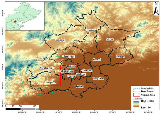
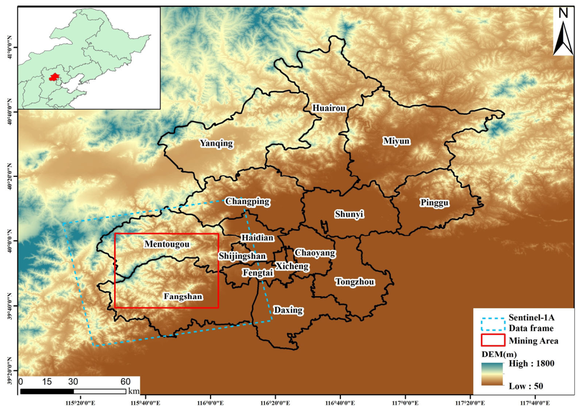
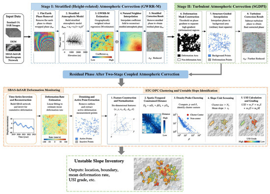
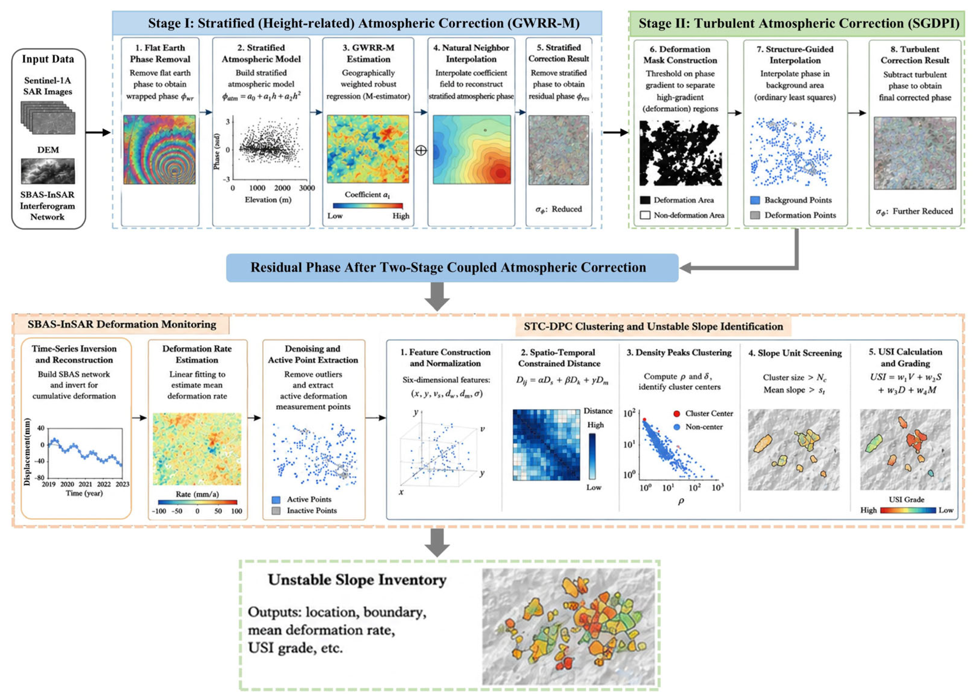
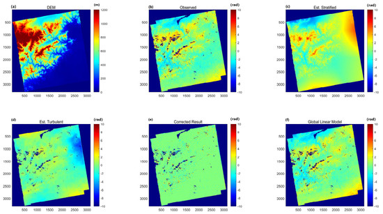
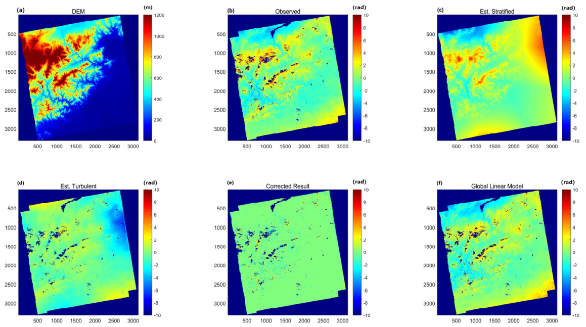
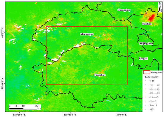
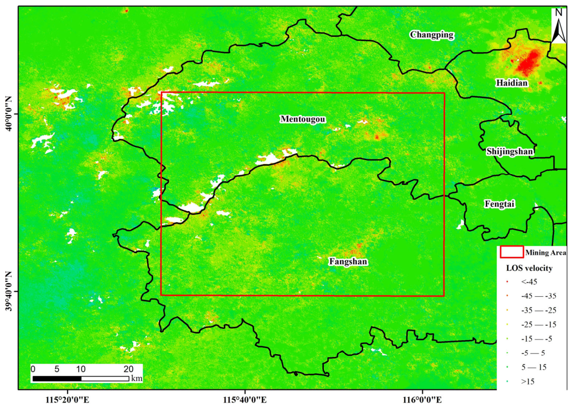
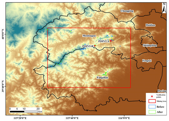
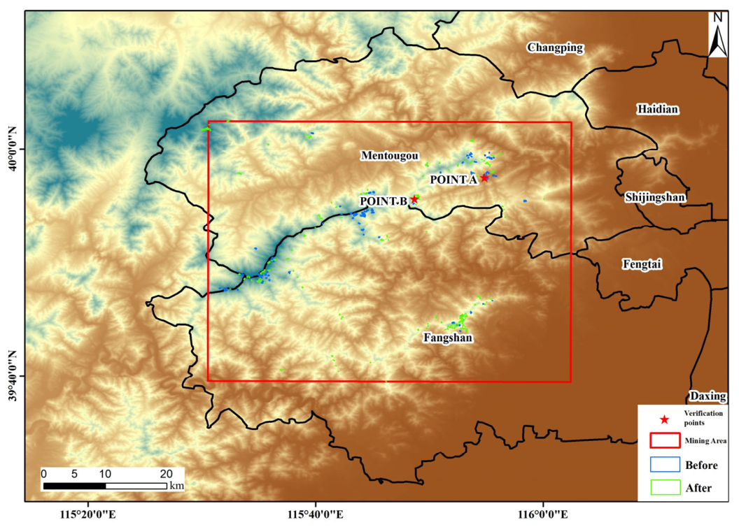
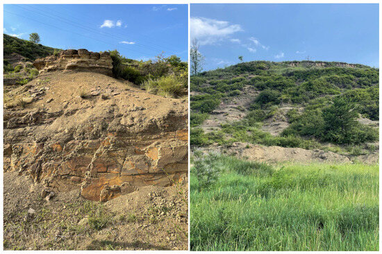
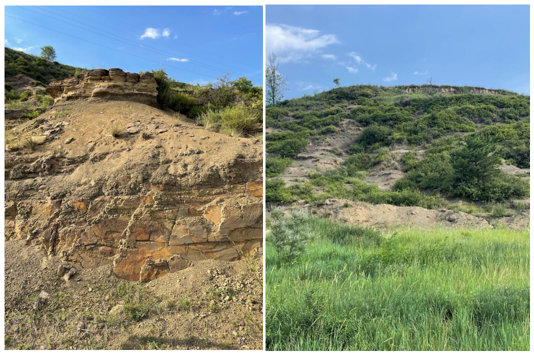
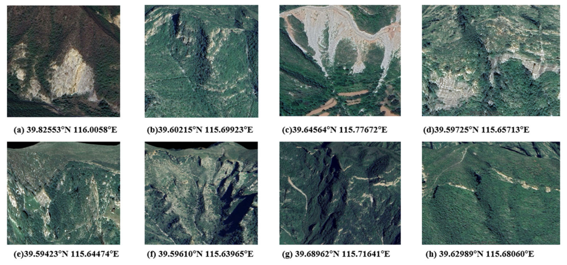
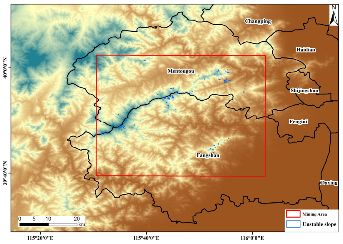
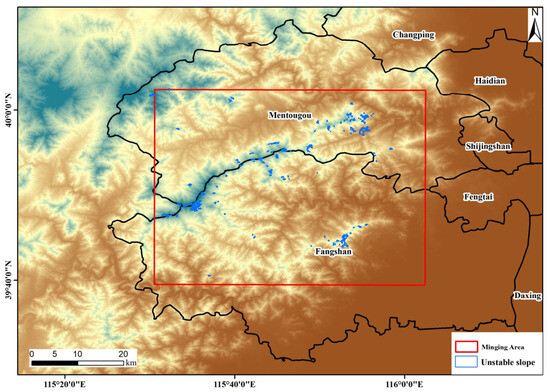
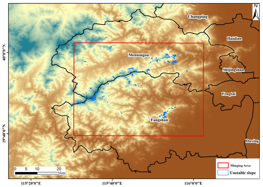

Disclaimer/Publisher’s Note: The statements, opinions and data contained in all publications are solely those of the individual author(s) and contributor(s) and not of MDPI and/or the editor(s). MDPI and/or the editor(s) disclaim responsibility for any injury to people or property resulting from any ideas, methods, instructions or products referred to in the content. |
© 2026 by the authors. Licensee MDPI, Basel, Switzerland. This article is an open access article distributed under the terms and conditions of the Creative Commons Attribution (CC BY) license.