Article

Convolutional Neural Networks in the Diagnosis of Colon Adenocarcinoma

1
Institute of Applied Sciences and Intelligent Systems (ISASI), National Research Council (CNR) of Italy, 73100 Lecce, Italy
2
Dipartimento di Ingegneria per L’Innovazione, Università del Salento, 73100 Lecce, Italy
3
Clinica Mediterranea, 80122 Naples, Italy
4
Italo Foundation, 20146 Milano, Italy
5
Department of Translational Medical Sciences, University of Naples Federico II, 80131 Naples, Italy
*
Author to whom correspondence should be addressed.
AI 2024, 5(1), 324-341; https://doi.org/10.3390/ai5010016
Submission received: 9 November 2023 / Revised: 5 January 2024 / Accepted: 24 January 2024 / Published: 29 January 2024

Abstract

:
Colorectal cancer is one of the most lethal cancers because of late diagnosis and challenges in the selection of therapy options. The histopathological diagnosis of colon adenocarcinoma is hindered by poor reproducibility and a lack of standard examination protocols required for appropriate treatment decisions. In the current study, using state-of-the-art approaches on benchmark datasets, we analyzed different architectures and ensembling strategies to develop the most efficient network combinations to improve binary and ternary classification. We propose an innovative two-stage pipeline approach to diagnose colon adenocarcinoma grading from histological images in a similar manner to a pathologist. The glandular regions were first segmented by a transformer architecture with subsequent classification using a convolutional neural network (CNN) ensemble, which markedly improved the learning efficiency and shortened the learning time. Moreover, we prepared and published a dataset for clinical validation of the developed artificial neural network, which suggested the discovery of novel histological phenotypic alterations in adenocarcinoma sections that could have prognostic value. Therefore, AI could markedly improve the reproducibility, efficiency, and accuracy of colon cancer diagnosis, which are required for precision medicine to personalize the treatment of cancer patients.

1. Introduction

Colorectal carcinoma (CRC) is a well-characterized heterogeneous disease induced by different tumorigenic modifications in colon cells [1]. CRC contains several stromal and epithelial tissue types representing different differentiation stages, including benign residual adenoma, that collectively support carcinogenesis and serve as diagnostic components. Malignant transformation modifies the morphology of the intestinal crypt structure in the mucosa, replacing it with irregular tissue composed of cells with an increased nucleus/cytoplasm ratio, thereby disrupting the normal glandular structure of colon tissue [2].
Malignant transformation of immortalized cells in high-grade adenomas is the earliest form of clinically relevant colorectal cancer, pT1, in which cancer cells have invaded the submucosa but not the muscular layer. At stage pT2, the tumor has invaded through muscularis propria, the muscle layer, but it has not migrated to nearby lymph nodes or distant organs. Stage pT3 cancer has grown through the muscularis propria into the subserosa, a thin layer of connective tissue covering the muscle layer, and often invades into tissues surrounding the colon. At stage pT4, the tumor has grown through all layers of the colon, invaded the visceral peritoneum, and commonly metastasized to distant organs. Metastatic colon cancer typically invades through the muscularis mucosa into the submucosa and occasionally into the proximity of blood vessels. A second distinctive histological feature indicating metastasis is a desmoplastic reaction in the tumor stroma, and the third nominator of possible metastasis is the presence of necrotic debris in the glandular lumina [3,4,5].
In addition to staging, colon cancer is classified based on grading, which is determined by the stage of undifferentiation of the cells, i.e., the number of abnormalities in the cellular phenotype. Colon cancer is usually divided into three grades: well-differentiated (low grade, G1), moderately differentiated (intermediate grade, G2), and poorly differentiated (high grade, G3) [6]. A well-differentiated (G1) adenocarcinoma has conserved more than 95% of the normal glandular formation, whereas in moderately differentiated colon cancer (G2), the colon has 50–95% glandular formation, and poorly differentiated (G3) has less than 50% glandular formation [6].
The current histologic diagnosis has several deficiencies, which may affect the therapy decisions, consequent recovery, and survival of patients. Artificial intelligence (AI), especially recently developed computer vision methodologies based on deep learning and digital pathology, can recognize and mark pixels in the image, distinguish the pixels based on their characteristics, and detect the differences and grade cancers [7]. The computer-based analysis of colon digital histologic images involves different tasks [7,8], such as the normalization of histologic staining, to match the staining colors with a given template to eliminate the variability of histological sample staining [9]. Other tasks include the segmentation of cells to identify cellular structures and organelles [10]; the division of tissues into the tumor, stroma, and adipose tissue [11]; the detection of the parameters indicating cancer progression, e.g., lymphocyte migration and cellular proliferation [12]; and the prediction of consequent survival by combining the information of patient’s age, gender, medical status, and physical condition [13].
In the current work, we used subclasses of artificial neural networks that learn directly from data: ResidualNet, DenseNet, EfficientNet, and Squeeze-and-ExcitationNet. Neural networks are simplified artificial models of human brain physiology that can be used for the analysis of histologic sections in the diagnosis of cancer. The CNNs used in this work were combined as ensembles to improve the stability and predictivity of the final output [14]. To further improve machine learning, we introduced transformer models to adopt the mechanism of cognitive attention and classify the observed and unobserved data by predicting the latter [15]. Lastly, we introduced an optimal network model to improve network performance [16].
To train the algorithm, we used the CRC-Dataset [17], extended CRC dataset [1], and GLA dataset [18] that contain 484 visual fields, which were then further divided into subfigures. The trained algorithm was used to diagnose patients with low-grade (G1), intermediate-grade (G2), and high-grade (G3) colon adenocarcinomas. The algorithm demonstrated high accuracy in the diagnosis of colon cancer.
The innovation of this study is to propose a two-stage CNN model for glandular region classification that mimics the work of a pathologist. In this new data flow, we characterized which CNN model is most suited to extract information from glandular regions and how different models could be combined to further improve cancer staging capabilities.
The main contributions of this study are as follows:
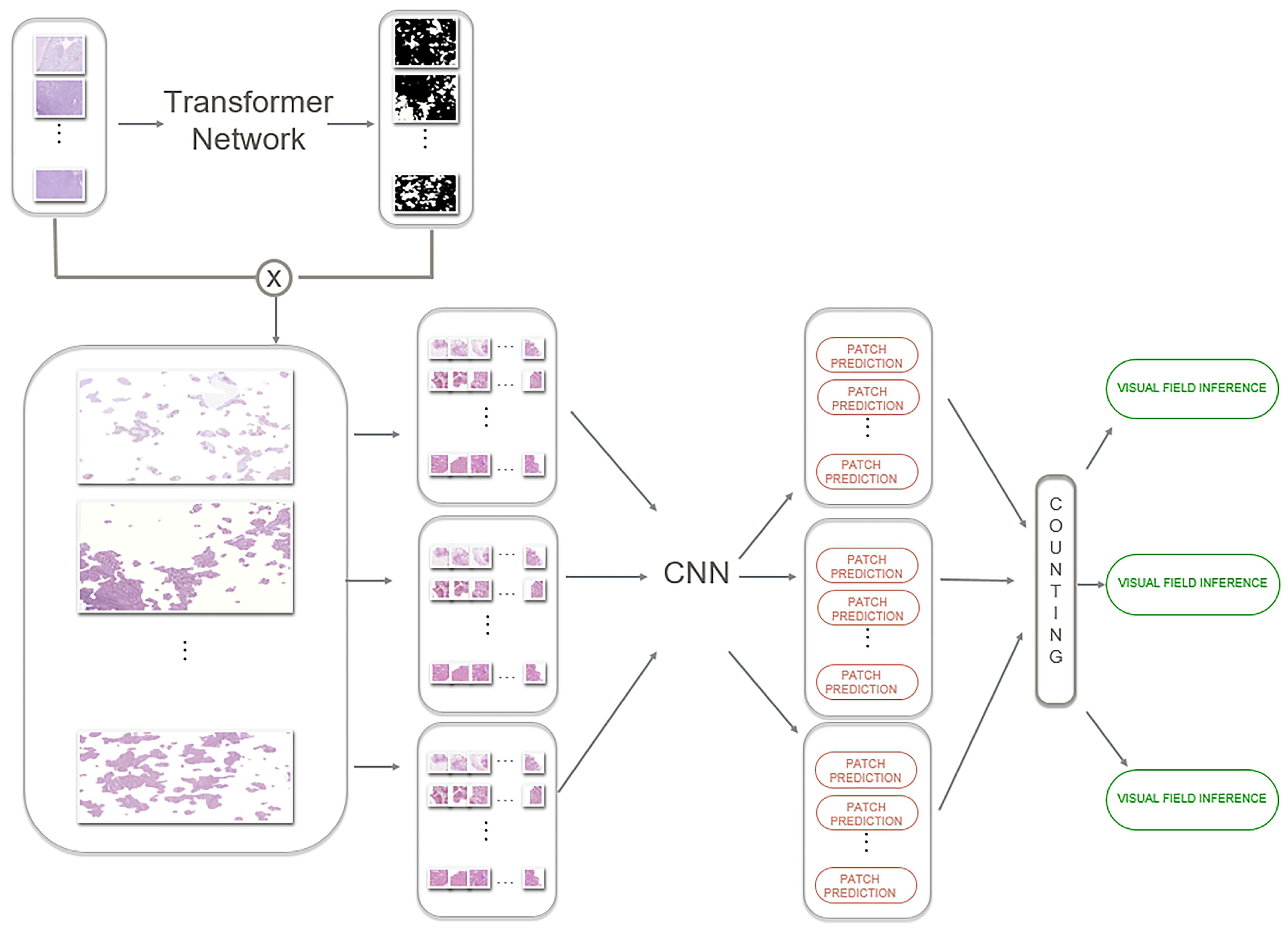
  • This is an innovative two-stage pipeline approach, as opposed to previous approaches that grade carcinoma initiating from patches containing glandular regions and other indiscriminative areas (e.g., epithelium).
  • This is among the first clinical approaches of this type of pipeline. This study provides early evidence of its suitability for clinical practice and a systematic report of the capabilities of the proposed model.
  • In this new data flow, we attempted to understand which CNN model is most suited to extract information from glandular regions and how different models could be combined to further improve cancer staging capabilities. The current work represents a few attempts at applying machine learning strategies in actual clinical practice for colon cancer grading.
  • This is among the first attempts to concentrate classification only on glandular regions, which shows a focus of attention similar to the diagnosis of a pathologist. This is one of the most important contributions of the self-attention mechanism learning approach.

2. Related Work

Extracting information from small datasets of biased and tagged data is challenging because of variation and similarities between or within classes that result from the continuum created by the various grade levels. Shallow classifiers and manually created features were the mainstays of early attempts to use AI in colon cancer grading [19]. Recently, deep learning-based methods have proven to be superior in the grading of colon cancer because of computational and memory constraints; CNNs are typically used for representation learning from small image patches (e.g., 224 × 224) recovered from digital histological images [20].
To aggregate predictions and model the reality that not all patches will be discriminative, patch-level classification results must be aggregated [21]. Based on images of tumor samples, the authors of [20] trained a deep network to forecast colorectal cancer outcomes by combining convolutional and recurrent architectures. In a novel cell graph convolutional neural network (CGC-Net), the increased accuracy of computational models was achieved by integrating contextual information with feature sharing and learning dependencies across and between scales using a long short-term memory (LSTM) unit [22].
In this model, large images are presented as a graph, where each node is represented by a nucleus within the original image, and cellular interactions are indicated as edges between these nodes based on node similarity. More recently, a proposed method for learning histological images uses a local-aware region CNN (LR-CNN) to first train the local representation and then a representation aggregation CNN (RA-CNN) to aggregate contextual data [23].
However, because there is often an insufficient amount of data available for robust knowledge generalization, a recent study [24] examined multiple CNN architectures and demonstrated that classical network models created for image classification have higher performance than those incorporating domain-specific solutions. Furthermore, it was shown that the EfficientNet-B1 and EfficientNet-B2 architectures [25] perform better than all previous state-of-the-art methods for CRC grading. Lastly, CNN has recently been suggested to effectively assist in completing knowledge extraction tasks from large histological images when an attention mechanism is applied in parallel to capture key features that aid network categorization [26].
Most of the existing approaches have been tested on benchmark datasets [27,28], but it is unclear whether there are enough data to support their implementation in current evidence-based clinical practice [29]. Advanced studies reporting clinical trials have been conducted only for colon tissue or nucleus segmentation [30].

3. Methods

The main aim of this paper was to introduce a two-stage colon adenocarcinoma grading pipeline. The first stage aimed at segmenting glandular regions, whereas the second step was devoted to grading regions retained after segmentation. The second contribution was to merge the advantages of CNN and transformer architectures. Transformers were exploited for the segmentation step to precisely determine glandular boundaries to be supplied to the following multiclass grading problem, relying on the CNN to extract local patterns of cells’ configurations.

3.1. Patients

Human adenocarcinoma sections were stained with hematoxylin–eosin (Sigma-Aldrich, St. Louis, MO, USA) and prepared for microscopy and imaging (Leica DMI3000B microscope and Leica Application Suite X 1.1.0.12420 camera software, Leica, Wetzlar, Germany). The ethical permissions for the study were approved by the Monaldi Hospital ethical committee, the University of Naples Federico II ethical committee, and the Clinica Mediterranea ethical committee. Inform consent was asked from all patients.

3.2. Development of the Algorithm

In this study, a transformer-based model with an additional control mechanism in the self-attention module was preliminarily exploited to understand discriminative regions in large histological images.
The development of the deep learning diagnosis tool was performed a workstation equipped with an Intel(R) Xeon(R) E5-1650 @ 3.20 GHz CPU, one GeForce GTX 1080 Ti with 11 GB of RAM GPU, and the Ubuntu 16.04 Linux operating system. In this study, we used the most advanced architectures that have demonstrated significant performance in the ImageNet Large Scale Visual Recognition Challenge (ILSVRC) [19] and in solving vanishing gradient architectures caused by the analysis of several layers. In the selection process, we used a generalization combined with a low memory footprint during the interference in the related problems [31]: ResidualNet [32], DenseNet [33], Squeeze-and-ExcitationNet [34], and EfficientNet [35]. All networks were modified to adapt to a 3-class inference problem.
Data augmentation was applied to the original data in terms of operations of horizontal and vertical image flipping, rotation with a value of ±45° and ±90°, and shearing between −20° and 20°. For the validation set, we used a stochastic gradient descent optimizer with a learning rate of 0.001, momentum of 0.9, and weight decay of 0.001. For the training process, we used an early stopping strategy of 22 epochs (the number of times a dataset passes through an algorithm), with a maximum of 100 training epochs.
In this work, we used a RegNet architecture, a network design space needed for architectures to function, integrating the Squeeze-and-ExcitationNet across a wide range of floating point operations (FLOPs) per second regimes, i.e., the number of multiply–add operations per processed image. For the identification of the generated models, the corresponding FLOP regime was marked on the basis of its construction; e.g., RegNetY-400MF means that the RegNet architecture built a 400 mega-FLOP model.
To extract information from both the entire image and local patches, where finer details can be found, visual fields were fed as inputs to a transformer network that combines local and global training [12]. They employ a deep local branch and a shallow global branch to gather data for their local–global training strategy. The feature maps, which were extracted from the first convolution block with three convolution layers each followed by batch normalization and ReLU activation, were fed into both branches. The encoder bottleneck was composed of two layers of multi-head attention layers, one operating along the width axis and the other along the height axis, after normalization and a 1 × 1 convolution layer.
Each multi-head attention block consisted of an axial attention layer. To create the output attention maps, the output from the multi-head attention blocks was concatenated, run through an additional 1 × 1 convolution, and then added to the residual input maps. The convolution layer, upsampling layer, and ReLU comprised the decoder block, consisting of two encoding blocks and two decoding blocks in the global branch. In the local branch, there were five encoding blocks and five decoding blocks.
In the grading of colon carcinomas, the transformer architecture aids in determining which regions of the large-scale histology images can aid in the discrimination of different grades of carcinomas by the subsequent CNN architectures, which enables higher performance using less data. The transformer was trained to extract glandular structures from the rest of the visual field content. These structures are currently considered to be one of the key biomarkers for determining tumor grade [17].
In subsequent training, the structures can produce matching binary masks that identify glandular regions on unseen visual fields. These masks can then be used to retain only the relevant portion for further processing by CNN models. EfficientNet architectures [10], which uniformly scale the width, depth, and resolution of the network using a compound coefficient, are most commonly used for CRC grading tasks.

3.3. Training of the Algorithm

For machine learning, we used three open-source datasets. Firstly, we used the CRC-Dataset [17], which comprises 139 visual fields extracted from 38 hematoxylin–eosin-stained whole-slide images with an average size of 4548 × 7520 pixels obtained at 20× magnification. These visual fields were classified into three different classes; normal tissue, low-grade cancer, and high-grade cancer, based on the histological structure of the glands. Second, the extended CRC dataset, which has been extracted from 68 hematoxylin–eosin-stained whole-slide images, consists of 300 visual fields with an average size of 5000 × 7300 pixels [1]. Third, the GLAs dataset [36] consists of 165 images derived from 16 hematoxylin–eosin-stained sections representing stage T3 or T4 colorectal adenocarcinoma. Because the histological images originate from different sources, the datasets exhibit high inter-subject variability in both stain distribution and tissue architecture. The digitization of these histological sections to whole-slide images was performed using a Zeiss MIRAX MIDI Slide Scanner with a pixel resolution of 0.465 μm. The whole-slide images were subsequently rescaled to a pixel resolution equivalent to 20× magnification. A total of 52 visual fields from both malignant and benign areas across the entire set of whole-slide images were selected to cover the tissue architectures. Manual annotation of glandular regions as normal, low grade, and high grade was used as a “ground truth” for training the transformer network (Table 1). Because of interobserver variation, G1 and G2 were combined to a low grade, and G3 was considered a high grade.

3.4. Diagnosis of Patients

The developed algorithm was used to diagnose images covering the whole tissue section (1824 × 1368 pixels, 20× magnification) of 11 patients with different stages of colon adenocarcinoma. From the images, we prepared a dataset consisting of 11,089 hematoxylin–eosin-stained images that were divided into 11 directories, each representing one patient (Table 2).
Correspondingly to datasets used for machine learning, the diagnosis aimed to classify the adenocarcinomas as well-differentiated (low grade), moderately differentiated (intermediate grade), and poorly differentiated (high grade). The selected patients represented advanced pT3 and pT4 stages of adenocarcinoma with neoplastic infiltration into neighboring tissues, excluding samples from patients 1 and 3. The sample from patient 1 was isolated from a liver metastasis, whereas patient 3 had a pathological stage pT1 adenocarcinoma with no metastasis. The dataset of image directories is available at https://dataset.isasi.cnr.it/2021/10/18/cnr-crc/ (accessed on 24 January 2024).
The main limitations of this study are as follows: (1) the number samples used for real clinical experimentation and (2) the necessity to start large training sessions when additional examples from different patients become available.

4. Results

4.1. Development of the Algorithm

Deep learning-based colon carcinoma grading is an emerging diagnostic method that can improve the overall grading accuracy in tumors with several grading levels and reduce person-related alterations in the diagnosis. To use artificial intelligence in patch-based approaches of histological diagnosis, tissue sections are generally divided into single patches, e.g., size 224 × 224 pixels, for the primary analysis, which are then combined to cover the whole section for classification of the informative content of each patch and for predictions to label the whole image. Deep CNNs have inherent inductive biases without the ability to calculate long-range dependencies, whereas transformer-based network architectures [37] developed for language tasks can be used for image segmentation analysis [38].
In this paper, a transformer-based model equipped with an additional control mechanism in the self-attention module was used to analyze discriminative regions in histological images. During the training process, the transformer gained binary masks, which marked the glandular regions used in the CNN model (Figure 1).
The algorithm comprised ResidualNet, DenseNet, Squeeze-and-ExcitationNet, and EfficientNet [32,33,34,35] architectures that minimize the vanishing problem and have high generalization capacity and a low memory footprint. ResidualNet addresses the vanishing gradient and training degradation problems by introducing a deep residual learning approach, in which each of the stacked layers of the entire network was analyzed using skip connections. Once ResidualNet had created the infrastructure, the DenseNet architecture was used to connect each layer in a feed-forward fashion, collecting information from all previous layers as input to all subsequent layers. Squeeze-and-ExcitationNet was used to improve the interdependences of the convolutional channels to emphasize the informative features and suppress irrelevant noise. EfficientNet was used to optimize and uniformly scale the network width, depth, and resolution.
Next, to reduce the inaccuracy and bias created by single neural networks, we assembled them as a Max-Voting ensemble and Argmax ensemble, which combine neural networks that have been trained with different parameters [20]. The Max-Voting ensemble combines the network predictions from each patch and assigns the most voted label to the final result. The Argmax ensemble computes the total number of patches produced by the combined networks and assigns to each patch a vector of labels equal to the number of networks involved in the ensemble.

4.2. Training of the Algorithm

The training addressed two classifications: first, the binary problem to distinguish normal tissue from tumor tissue in which intermediate and high grades have been put together and considered as a unique class against the class including only examples of lower-grade cancer, and second, the ternary three-class problem of grading tissues to normal tissue, low-grade cancer, and high-grade cancer. Because all the previous approaches have used cross-validation of the same split to avoid data leakage (i.e., the patches of each subject were in the same fold without using the subject for training or testing), we used three-fold cross-validation for a fair comparison of existing approaches.
To avoid overfitting, we split 92 visual fields for fold 1, 92 visual fields for fold 2, and 89 visual fields for fold 3. From each visual field, we extracted 224 × 224-pixel non-overlapping size-16 patches, which were labeled according to the label of the corresponding visual field or the background. These were then used as inputs to the subsequent machine-learning strategies with a batch size of 16. The patch distribution per fold and class extracted from the extended CRC dataset are shown in Table 3. We excluded approximately 11% of patches representing the crypts or lamina propria from further analysis because of their irrelevant informative content. These background batches had an average radiometric value higher than 235 in the three-color channels and appeared white in the images.
The metrics used for the evaluation were average accuracy, which refers to the correct classification percentage of the visual fields, and weighted accuracy, which is the sum of the accuracies in each class weighted by the number of samples in that class. For each fold j in the range [1, k] (k = 3 in the following experiments), the average accuracy was computed as follows:
a c c j = i = 1 c T P i i = 1 c N i
Similarly, the weighted accuracy was computed as the average of
a c c j = i = 1 C T P i N i C
where C indicates the number of classes (2 or 3), N i is the number of elements in class i, and T P i is the number of true positives for class i. Once the patches were analyzed with ResidualNet, DenseNet, Squeeze-and-ExcitationNet, and EfficientNet architectures, we combined them with the Max-Voting ensemble to improve the prediction result.
In the training process, we first analyzed the average and weighted classification of the binary and ternary three-class problems, and then the variance of the folding scores on the extended CRC dataset (Table 4).
ResNet50 was used as a PIVOT tool to verify the implementation of the data handling process. EfficientNet-B2 and DenseNet121 models demonstrated the highest accuracy scores for both the binary and ternary three-class problems. The training time for EfficientNet-B2 was 477 min, for DenseNet121 746 min, for EfficientNet-B0 224 min, for EfficientNet-B1 452 min, for EfficientNet-B3 481 min, EfficientNet-B4 518 min, for EfficientNet-B5 677 min, for EfficientNet-B7 1188 min, for ResidualNet50 276 min, for ResidualNet152 493 min, and for Squeese-and-ExitationNet-ResidualNet50 4496 min.
Next, we trained the classification and grading on the extended CRC dataset (Table 5). When optimally designed network models, RegNetY-4.0GF and RegNetY-6.4GF, were used, the training time demonstrated improved performance of 273 min and 337 min, respectively.
To train the images and binary mask of the transformer network, we used GLA dataset histological images. Subsequently, the learned configuration was used to extract a binary mask for the extended CRC dataset. The patches corresponding to the predicted glandular regions were then used as inputs to the subsequent CNN-based colon carcinoma grading (Figure 2).
The workstation used for the experiments had an Intel(R) Xeon(R) CPU E5-1650 @ 3.20 GHz, a GeForce GTX 1080 Ti GPU, 11 GB of RAM-GPU, and SO Ubuntu 16.04 Linux. All the examined CNNs were optimized by initiating from the pre-trained ImageNet models that come with the reference implementations. Next, we employed data augmentation techniques to restrict the number of visual fields. More specifically, horizontal and vertical flipping, as well as rotation using a random value, was selected from the list (−90, −45, 45, 90), whereas random x-axis shearing ranged from −20 to 20 degrees.
Lastly, we used learning rate = 0.001, momentum = 0.9, weight decay = 0.001, batch = 16 parameters, an early stopping strategy of 10 epochs on the validation set with a maximum number of 100 training epochs, and the stochastic gradient descent (SGD) optimizer, followed by the training configuration for the transformer architecture, which included an Adam optimizer, a batch size of 4, and a learning rate of 0.001. The network was trained for 400 epochs.
To analyze and mark the background from the experimental batches, we analyzed the per fold and class of the patch distribution, which were extracted from the visual fields of the extended CRC database (Table 6). The analysis reduced approximately 46% of (1) sporadic noise regions and (2) regions delineating the border of the experimental batches in the initial study area. As a result, the workload of the CNN models was reduced from 89% to 40%. Importantly, the reduction affected only the number of patches contributing to the final labeling, whereas the number (300) of visual fields classified in the extended CRC dataset remained the same (Supplemental Table S1).
The results obtained from patch distribution were confirmed by quantitative results (Supplemental Table S2) that showed grading data using transformer networks to discard discriminative regions.
The use of the transformer network corroborated the CNN classification for all models, most prominently for EfficientNet, and improved the performance. The EfficientNet-B1 model demonstrated the highest performance in binary classification, whereas the EfficientNet-B2 model was the most efficient in solving the ternary three-class problem. Furthermore, the use of the transformer network reduced the number of patches included in the analysis, consequently shortening the training time. The training times of T + EfficientNet-B1 and T + EfficientNet-B2 were 121 and 133 min, respectively, demonstrating a marked 70% reduction compared with to training without the transformer network. The ensembles built for testing the extended CRC dataset demonstrated robust performance in analyzing the average and weighted accuracy of the ternary three-class problem (Table 6a).
The preliminary application of the transformer network allowed the analysis chain (Figure 1) to utilize the ensemble of networks to gain increased accuracy in colon carcinoma grading in the extended CRC dataset. The ensembling markedly increased the scores compared with the performance of single network architectures (Table 6b), most prominently ensembling EfficientNet-B1, EfficientNet-B2, and RegNetY16GF E11 (Table 6a), which resulted in the highest performance in both binary and ternary classification problems.
Finally, we performed an ablation study to assess the contribution of transformer architecture. In the same pipeline, a CNN-based segmentation model was used instead of a transformer in the first stage of the pipeline. For this purpose, we used a faster region-based convolutional neural network (fRCNN) architecture for segmentation with a ResNet-101 feature extraction backbone, as previously reported in [39]. The network was trained on the GLAs dataset and validated on the extended CRC. The extracted patches were then split in folds and given as inputs to the E11 ensemble (Table 6). The binary (average and weighted) and ternary (average and weighted) classification outcomes were 97.21 ± 0.35, 96.32 ± 3.41, 88.95 ± 3.45, and 87.88 ± 2.45, respectively. The data suggested that by exploiting CNN-based segmentation, the classification accuracy decreased in cases in which the proposed transform was used for the segmentation of glandular regions.

4.3. Diagnosis of Patients

The neural networks graded cancer using images (20× magnification) divided into patches. For each visual field, the proposed pipeline created a map in which colon grading in each selected patch was highlighted by the transformer (green, blue, and red for grades 0, 1, and 2, respectively) (Figure 3).
To quantitatively validate the deep learning procedure, the developed network was tested using our colon adenocarcinoma patient dataset. A pathologist diagnosed the patients based on their personal data (gender, age, medical history), surgical information, microsatellite analysis, oncogene (EGFR, NRAS, KRAS, BRAS) mutation analysis, and histological information, such as glandular structure, tumor budding, inflammatory cell staining, local invasion and infiltration, lymph node/liver metastasis, mismatch protein staining, and differentiation marker staining (Table 7).
Table 8 shows a comparison of the grading performed by the pathologist and the algorithm.
Patient 1′s sample was isolated from a hepatic metastasis derived from colon adenocarcinoma. Histopathological grading suggested a moderately differentiated tumor, whereas AI predicted poorly differentiated grading. The discrepancy between the histopathological diagnosis and algorithm-predicted grading of the patient 1 tumor may suggest that the aggressive metastasized cancer had been able to maintain the moderately differentiated glandular status even at a distant organ but had gained other phenotypic characteristics of aggressive cancer. Patient 2 had pT4 stage adenocarcinoma that had infiltrated the omental tissue. The pathological stage and histological grading, which were poorly differentiated, supported the grading calculated by the ensemble transformer networks. Patient 3, diagnosed with pT1 stage cancer without metastasis, demonstrated well-differentiated adenocarcinoma by both the pathologist and the network. The data from patient 3 demonstrated that the algorithm created in the current study can separate well-differentiated cancers from advanced-stage tumors.
The grading diagnosis of patient 4, suggesting poorly differentiated stage pT3 adenocarcinoma, was the same as that by the pathologist and algorithm. The patient had intratumoral cancer cell migration that reached the muscular layer and perivisceral fat. The histopathological diagnosis of patient 5 suggested moderately differentiated colon adenocarcinoma, whereas the transformer network-predicted analysis suggested poorly differentiated cancer. Interestingly, the predicted diagnosis was a borderline case in which 48% of the analyzed high-power fields suggested moderately differentiated and 52% suggested poorly differentiated grading. The patient had 19 metastatic lymph nodes and intratumoral infiltration of neoplastic cells into the perivisceral fat, indicating the progression of tumorigenesis toward a more aggressive phase. In addition, the diagnosis suggested a rare colloid adenocarcinoma, which results in a lower 5-year survival (71%) rate than the survival rate of a common form of adenocarcinoma (81%). Therefore, the algorithm predicted differentiation grading, which may have identified morphological features characteristic of high-risk cancer and decreased survival.
Similarly, for patient 5, the algorithm-predicted differentiation of patient 6 was divided between moderately differentiated (52%) and poorly differentiated grades (48%). The histopathological diagnosis of moderately differentiated adenocarcinoma was based on the invasion of neoplastic cells into the muscle layer and visceral fat and metastasis in one lymph node. Therefore, the algorithm-predicted diagnosis may suggest that the tumor is transitioning from a moderately to poorly differentiated grade. Patients 7, 8, and 9 were all diagnosed with poorly differentiated adenocarcinoma by both the histological analysis and transformer network calculation.
The grading of adenocarcinoma in patient 10 was diagnosed as moderately differentiated by histopathological analysis. However, the neoplastic region had more than ten tumor buds, and the transformed cells had filtrated to the muscular layer and visceral fat, thereby suggesting a high risk of vascular metastasis, although no lymphovascular infiltration was observed. The algorithm predicted grading and a poor differentiation level, thus challenging the histological diagnosis, which may suggest the presence of morphological characteristics other than changes in gland formation. According to histological grading analysis, patient 11 had a poorly differentiated adenocarcinoma that had metastasized to two nearby lymph nodes and the liver, demonstrating a highly aggressive advanced disease stage. Histological analysis detected neoplastic infiltration into the muscle layer and visceral fat. However, nearly all images, 74%, diagnosed by AI suggested a moderately differentiated grading for the tumor (Table 8).

5. Discussion

Most colon adenocarcinomas have residual adenoma regions, illustrating a high degree of intratumoral heterogeneity of CRCs that complicates histological diagnosis. The conventional diagnosis of colon cancer is based on endoscopic, radiological, and histopathological images [40]. Histological sample isolation by endoscopic biopsy or polypectomy for the initial diagnosis of colon adenocarcinoma may result in compromises caused by superficial or poorly oriented tissue collection. In addition, grading based on glandular differentiation is sensitive to artifacts caused by the subjective definition of poorly differentiated CRC, the inability to apply grading of CRC histotypes other than adenocarcinoma not otherwise specified (adenocarcinoma NOS), the dependence of grading analysis on microsatellite instability, and inter- and intra-observer variability, especially between G1 and G2 grading [41,42].
While colon cancer grading refers to the aggressiveness of the cancer, tumor staging indicates the size and spread of the tumor. Although tumor staging has its weaknesses, particularly in pT3 and pT4 cancers, it remains the most significant prognostic method in deciding the clinical treatment of a patient [6,43]. However, this is hampered by peritoneal involvement, which causes marked diagnostic variation even within the same tumor stage [44]. Based on peritoneal penetration, stage pT4 colon adenocarcinoma is divided into pT4a, penetration to the visceral peritoneum, and pT4b, penetration to adjacent organs, both of which have a high probability of developing into peritoneal metastasis. The probability of pT4 stage cancer developing peritoneal metastasis has significant variability, from 8% to 50%, because of the heterogeneity of pT4 adenocarcinomas [45]. Therefore, tumor staging is fortified by lymph node metastasis staging to support the prognostic value of the diagnosis, which is commonly subjective, poorly reducible, and often affected by cancer cell clusters in the pericolic fat disconnected from the primary tumor (tumor deposits), which can be satellite tumor nodules or lymph node metastases [45].
Tumor budding (cancer cell aggregates in the invasive part of tumor stroma) has significant prognostic value in predicting lymph node metastasis, local recurrence, and vascular invasion [45]. The cells in the aggregates have been demonstrated to have reduced epithelial marker cytokeratin staining and increased mesenchymal vimentin positivity, suggesting epithelial–mesenchymal transition with subsequently acquired increased invasive potential, cancer stem cell characteristics, and resistance to cancer drugs [46]. Vascular invasion observed at tumor buds identifies an increased risk of poor survival but has high interobserver variability, especially when the diagnosis relies only on hematoxylin–eosin staining of the histological sections without using CD31 or CD34 endothelial cell antibodies [18]. Another important prognostic marker suggesting aggressive features and poor prognosis is the perineural invasion of cancer cells around nerve fibers and nerve sheaths. It does not correlate with the pT staging classification, although it can correlate with vascular invasion and lymph node metastasis [47].
Histological diagnosis can be strengthened with molecular pathology to identify microsatellite instability, chromosomal instability, CpG island methylation phenotype, and mutations in EGFR, KRAS, NRAS, and BRAF oncogenes. Molecular pathology is important in the support of histological diagnosis, the identification of hereditary forms of colon tumorigenesis, and treatment decisions [48].
Although the current diagnosis of colon cancer relies on several different techniques, there is a need for further development of an examination methodology to create more reliable prognostic and predictive diagnoses to support the therapy options. In our study, the diagnosis of histological patient samples (Table 7) using the developed network architectures corroborates previous observations that the current grading of colon adenocarcinoma based on glandular differentiation is not adequately accurate [49]. The discrepancy between the histopathological diagnosis and algorithm-predicted grading of the tumors of patients 1, 5, 10, and 11 suggests that during the deep learning process, the network architectures omitted additional criteria from the morphology of hematoxylin–eosin-stained tissue sections that characterize aggressive cancer type. The data demonstrate that CNNs equipped with transformers can perform the diagnosis with similar accuracy to a pathologist using only images of hematoxylin–eosin-stained tissue sections. Therefore, histopathological digital image patch processing by computer vision deep learning could provide healthcare professionals with a reproducible and reliable automatic diagnosis of colon carcinoma.
Although CNNs have been used for image segmentation, they originally learned only short-range spatial dependencies [50]. The segmentation approach based on transformers, which relies on self-attention mechanisms and pre-training between neighboring image patches without any convolution operations, has been demonstrated to be more efficient than CNNs [51]. Other advantages include the ability of transformers to introduce a loss of feature resolution that is absent in CNN-based analysis and an additional control mechanism in the self-attention module that improves the image segmentation in medical applications [52]. However, transformer-based models function adequately only when they are trained on large-scale datasets or when a set of pre-learned weights is available.
The solution proposed demonstrated a higher potential for two- and three-class classification tasks than previously published solutions. The data demonstrated higher performance in achieving classification scores for the transformer networks EfficientNet-B1, EfficientNet-B2, and RegNetY16GF. The accuracy scores showed a significant increase of 2% for the average two classes, 2.08% for the weighted two classes, 3.58% for the average three classes, and 3.89% for the weighted three classes (Table 9).
In conclusion, in this study, we developed a novel AI-based colon cancer diagnostic method. For this purpose, we used manually and automatically designed convolutional architectures in classification tasks in the deep learning of colon adenocarcinoma grading from histological images. Transformer architectures further introduced an attention mechanism to highlight the most discriminative areas. Finally, we tested the developed ensembling of networks using patient material. The data demonstrated a substantial improvement in the learning time and quality of the final diagnosis. The introduced machine learning strategies could provide healthcare professionals with a computational tool to objectively evaluate carcinoma, thereby avoiding a bias introduced by different circumstances.
The current data create a foundation for improved cancer diagnosis. Future research directions will address a larger recruitment of patients to allow for a better assessment of the proposed methodology. New end-to-end strategies will be studied, including few-shot and incremental learning strategies, to increase the amount of extracted knowledge in the process to avoid the need to restart training. Furthermore, knowledge and model distillation processes will be used to improve the transfer of knowledge from a large model to a smaller one, which could also be implemented in mobile and low-power devices, thereby enabling remote diagnoses for medical professionals. For the future improvement of visual convolutional networks, we will evaluate the proposed model in the diagnosis and prognosis of other pathologies, such as neuronal degeneration.

Supplementary Materials

The following supporting information can be downloaded at: https://www.mdpi.com/article/10.3390/ai5010016/s1, Supplemental Table S1. Patch distribution per fold and class in the transformer network. Supplemental Table S2. Results for the extended CRC dataset while integrating the transformer networks.

Author Contributions

Methodology, M.L., P.C., L.S., G.B., M.O.L. and C.D.; Software, M.L., P.C., L.S. and C.D.; Validation, M.L., P.C., L.S., F.C., G.B., M.O.L. and C.D.; Formal analysis, P.C., L.S., F.C., G.B. and C.D.; Investigation, M.L., G.B. and M.O.L.; Resources, F.C. and G.B.; Writing—original draft, M.L., P.C., M.O.L. and C.D.; Writing—review and editing, M.O.L.; Supervision, L.S. and C.D.; Project administration, F.C. and C.D.; Funding acquisition, M.O.L. All authors have read and agreed to the published version of the manuscript.

Funding

This research and APC was funded by Campania Region POR CUP B63D18000210007 and Future Artificial Intelligence Research—FAIR CUP B53C220036 30006 grant number PE0000013.

Institutional Review Board Statement

The study with patient samples was conducted in accordance with the Declaration of Helsinki and approved by the Institutional Review Board of the Clinica Mediterranea ethical committee, Naples, Italy, Monaldi Hospital ethical committee (Deliberazione del Direttore Generale n:o 1239), Naples, Italy, and by the University of Naples Federico II ethical committee (protocol number 394/19), Naples, Italy.

Informed Consent Statement

Informed consent was obtained from all subjects involved in the study.

Data Availability Statement

Data is contained within the article and Supplementary Material.

Conflicts of Interest

The authors declare no conflict of interest.

References

  1. Testa, U.; Pelosi, E.; Castelli, G. Colorectal cancer: Genetic abnormalities, tumor progression, tumor heterogeneity, clonal evolution and tumor-initiating cells. Med. Sci. 2018, 6, 31. [Google Scholar] [CrossRef]
  2. Hermanek, P. Colorectal carcinoma: Histopathological diagnosis and staging. Bailliere’s Clin. Gastroenterol. 1989, 3, 511–529. [Google Scholar] [CrossRef]
  3. Lanza, G.; Messerini, L.; Gafa, R.; Risio, M.; Gruppo Italiano Patologi Apparato Digerente (GIPAD); Societa Italiana di Anatomia Patologica e Citopatologia Diagnostica/International Academy of Pathology, Italian Division. Colorectal tumors: The histology report. Dig. Liver Dis. 2011, 43 (Suppl. S4), S344–S355. [Google Scholar] [CrossRef]
  4. Tong, Y.; Liu, D.; Zhang, J. Connection and distinction of tumor regression grading systems of gastrointestinal cancer. Pathol. Res. Pract. 2020, 216, 153073. [Google Scholar] [CrossRef]
  5. Cammarota, F.; Laukkanen, M.O. Mesenchymal Stem/Stromal Cells in Stromal Evolution and Cancer Progression. Stem Cells Int. 2016, 2016, 4824573. [Google Scholar] [CrossRef]
  6. Fleming, M.; Ravula, S.; Tatishchev, S.F.; Wang, H.L. Colorectal carcinoma: Pathologic aspects. J. Gastrointest. Oncol. 2012, 3, 153–173. [Google Scholar] [CrossRef] [PubMed]
  7. Deng, S.; Zhang, X.; Yan, W.; Chang, E.I.; Fan, Y.; Lai, M.; Xu, Y. Deep learning in digital pathology image analysis: A survey. Front. Med. 2020, 14, 470–487. [Google Scholar] [CrossRef] [PubMed]
  8. Salvi, M.; Acharya, U.R.; Molinari, F.; Meiburger, K.M. The impact of pre- and post-image processing techniques on deep learning frameworks: A comprehensive review for digital pathology image analysis. Comput. Biol. Med. 2021, 128, 104129. [Google Scholar] [CrossRef] [PubMed]
  9. Ciompi, F.; Geessink, O.; Bejnordi, B.E.; de Souza, G.S.; Baidoshvili, A.; Litjens, G.; van Ginneken, B.; Nagtegaal, I.; van der Laak, J. The Importance of Stain Normalization in Colorectal Tissue Classification with Convolutional Networks. In Proceedings of the 2017 IEEE 14th International Symposium on Biomedical Imaging (ISBI 2017), Melbourne, Australia, 18–21 April 2017; pp. 160–163. [Google Scholar] [CrossRef]
  10. Wang, E.K.; Zhang, X.; Pan, L.; Cheng, C.; Dimitrakopoulou-Strauss, A.; Li, Y.; Zhe, N. Multi-Path Dilated Residual Network for Nuclei Segmentation and Detection. Cells 2019, 8, 499. [Google Scholar] [CrossRef] [PubMed]
  11. Tsai, M.J.; Tao, Y.H. Deep Learning Techniques for the Classification of Colorectal Cancer Tissue. Electronics 2021, 10, 662. [Google Scholar] [CrossRef]
  12. Swiderska-Chadaj, Z.; Pinckaers, H.; van Rijthoven, M.; Balkenhol, M.; Melnikova, M.; Geessink, O.; Manson, Q.; Sherman, M.; Polonia, A.; Parry, J.; et al. Learning to detect lymphocytes in immunohistochemistry with deep learning. Med. Image Anal. 2019, 58, 101547. [Google Scholar] [CrossRef] [PubMed]
  13. Gupta, P.; Chiang, S.F.; Sahoo, P.K.; Mohapatra, S.K.; You, J.F.; Onthoni, D.D.; Hung, H.Y.; Chiang, J.M.; Huang, Y.; Tsai, W.S. Prediction of Colon Cancer Stages and Survival Period with Machine Learning Approach. Cancers 2019, 11, 2007. [Google Scholar] [CrossRef] [PubMed]
  14. Zhang, L.; Suganthan, P.N. Visual Tracking With Convolutional Random Vector Functional Link Network. IEEE Trans. Cybern. 2017, 47, 3243–3253. [Google Scholar] [CrossRef] [PubMed]
  15. Khan, S.; Naseer, M.; Hayat, M.; Zamir, S.W.; Khan, F.S.; Shah, M. Transformers in Vision: A Survey. ACM Comput. Surv. 2022, 54, 1–41. [Google Scholar] [CrossRef]
  16. Radosavovic, I.; Johnson, J.; Xie, S.N.; Lo, W.Y.; Dollár, P. On Network Design Spaces for Visual Recognition. In Proceedings of the 2019 IEEE/CVF International Conference on Computer Vision (ICCV), Seoul, Republic of Korea, 27 October 27–2 November 2019; pp. 1882–1890. [Google Scholar] [CrossRef]
  17. Awan, R.; Sirinukunwattana, K.; Epstein, D.; Jefferyes, S.; Qidwai, U.; Aftab, Z.; Mujeeb, I.; Snead, D.; Rajpoot, N. Glandular Morphometrics for Objective Grading of Colorectal Adenocarcinoma Histology Images. Sci. Rep. 2017, 7, 16852. [Google Scholar] [CrossRef] [PubMed]
  18. Liang, P.; Nakada, I.; Hong, J.W.; Tabuchi, T.; Motohashi, G.; Takemura, A.; Nakachi, T.; Kasuga, T.; Tabuchi, T. Prognostic significance of immunohistochemically detected blood and lymphatic vessel invasion in colorectal carcinoma: Its impact on prognosis. Ann. Surg. Oncol. 2007, 14, 470–477. [Google Scholar] [CrossRef]
  19. Altunbay, D.; Cigir, C.; Sokmensuer, C.; Gunduz-Demir, C. Color Graphs for Automated Cancer Diagnosis and Grading. IEEE Trans. Biomed. Eng. 2010, 57, 665–674. [Google Scholar] [CrossRef]
  20. Hou, L.; Samaras, D.; Kurc, T.M.; Gao, Y.; Davis, J.E.; Saltz, J.H. Patch-based Convolutional Neural Network for Whole Slide Tissue Image Classification. In Proceedings of the 2016 IEEE Conference on Computer Vision and Pattern Recognition (CVPR), Las Vegas, NV, USA, 27 June–30 June 2016; pp. 2424–2433. [Google Scholar] [CrossRef]
  21. Pei, Y.; Mu, L.; Fu, Y.; He, K.; Li, H.; Gu, S.X.; Liu, X.M.; Li, M.Y.; Zhang, H.M.; Li, X.Y. Colorectal Tumor Segmentation of CT Scans Based on a Convolutional Neural Network With an Attention Mechanism. IEEE Access 2020, 8, 64131–64138. [Google Scholar] [CrossRef]
  22. Zhou, Y.N.; Graham, S.; Koohbanani, N.A.; Shaban, M.; Heng, P.A.; Rajpoot, N. CGC-Net: Cell Graph Convolutional Network for Grading of Colorectal Cancer Histology Images. In Proceedings of the IEEE/CVF International Conference on Computer Vision Workshops, Seoul, Republic of Korea, 27 October–28 October 2019; pp. 388–398. [Google Scholar] [CrossRef]
  23. Zhan, Z.W.; Liao, G.L.; Ren, X.; Xiong, G.S.; Zhou, W.L.; Jiang, W.C.; Xiao, H. RA-CNN: A Semantic-Enhanced Method in a Multi-Semantic Environment. Int. J. Softw. Sci. Comput. Intell. 2022, 14, 1–14. [Google Scholar] [CrossRef]
  24. Shaban, M.; Awan, R.; Fraz, M.M.; Azam, A.; Tsang, Y.W.; Snead, D.; Rajpoot, N.M. Context-Aware Convolutional Neural Network for Grading of Colorectal Cancer Histology Images. IEEE Trans. Med. Imaging 2020, 39, 2395–2405. [Google Scholar] [CrossRef]
  25. Vuong, T.L.T.; Lee, D.; Kwak, J.T.; Kim, K. Multi-task Deep Learning for Colon Cancer Grading. In Proceedings of the 2020 International Conference on Electronics, Information, and Communication (ICEIC), Barcelona, Spain, 19–22 January 2020. [Google Scholar] [CrossRef]
  26. Sirinukunwattana, K.; Alham, N.K.; Verrill, C.; Rittscher, J. Improving Whole Slide Segmentation Through Visual Context—A Systematic Study. In Medical Image Computing and Computer Assisted Intervention—MICCAI 2018, Pt II; Springer: Cham, Switzerland, 2018; Volume 11071, pp. 192–200. [Google Scholar] [CrossRef]
  27. Tummala, S.; Kadry, S.; Nadeem, A.; Rauf, H.T.; Gul, N. An Explainable Classification Method Based on Complex Scaling in Histopathology Images for Lung and Colon Cancer. Diagnostics 2023, 13, 1594. [Google Scholar] [CrossRef]
  28. Bousis, D.; Verras, G.I.; Bouchagier, K.; Antzoulas, A.; Panagiotopoulos, I.; Katinioti, A.; Kehagias, D.; Kaplanis, C.; Kotis, K.; Anagnostopoulos, C.N.; et al. The role of deep learning in diagnosing colorectal cancer. Prz. Gastroenterol. 2023, 18, 266–273. [Google Scholar] [CrossRef]
  29. Bokhorst, J.M.; Nagtegaal, I.D.; Fraggetta, F.; Vatrano, S.; Mesker, W.; Vieth, M.; van der Laak, J.; Ciompi, F. Deep learning for multi-class semantic segmentation enables colorectal cancer detection and classification in digital pathology images. Sci. Rep. 2023, 13, 8398. [Google Scholar] [CrossRef]
  30. Reis, H.C.; Turk, V. Transfer Learning Approach and Nucleus Segmentation with MedCLNet Colon Cancer Database. J. Digit. Imaging 2023, 36, 306–325. [Google Scholar] [CrossRef] [PubMed]
  31. Gertych, A.; Swiderska-Chadaj, Z.; Ma, Z.; Ing, N.; Markiewicz, T.; Cierniak, S.; Salemi, H.; Guzman, S.; Walts, A.E.; Knudsen, B.S. Convolutional neural networks can accurately distinguish four histologic growth patterns of lung adenocarcinoma in digital slides. Sci. Rep. 2019, 9, 1483. [Google Scholar] [CrossRef]
  32. Chen, W.F.; Ou, H.Y.; Lin, H.Y.; Wei, C.P.; Liao, C.C.; Cheng, Y.F.; Pan, C.T. Development of Novel Residual-Dense-Attention (RDA) U-Net Network Architecture for Hepatocellular Carcinoma Segmentation. Diagnostics 2022, 12, 1916. [Google Scholar] [CrossRef]
  33. Zhang, Z.; Liang, X.; Dong, X.; Xie, Y.; Cao, G. A Sparse-View CT Reconstruction Method Based on Combination of DenseNet and Deconvolution. IEEE Trans. Med. Imaging 2018, 37, 1407–1417. [Google Scholar] [CrossRef]
  34. Eun, D.I.; Woo, I.; Park, B.; Kim, N.; Lee, A.S.; Seo, J.B. CT kernel conversions using convolutional neural net for super-resolution with simplified squeeze-and-excitation blocks and progressive learning among smooth and sharp kernels. Comput. Methods Programs Biomed. 2020, 196, 105615. [Google Scholar] [CrossRef] [PubMed]
  35. Marques, G.; Ferreras, A.; de la Torre-Diez, I. An ensemble-based approach for automated medical diagnosis of malaria using EfficientNet. Multimed. Tools Appl. 2022, 81, 28061–28078. [Google Scholar] [CrossRef] [PubMed]
  36. Sirinukunwattana, K.; Pluim, J.P.W.; Chen, H.; Qi, X.; Heng, P.A.; Guo, Y.B.; Wang, L.Y.; Matuszewski, B.J.; Bruni, E.; Sanchez, U.; et al. Gland segmentation in colon histology images: The glas challenge contest. Med. Image Anal. 2017, 35, 489–502. [Google Scholar] [CrossRef]
  37. Shakeel, P.M.; Burhanuddin, M.A.; Desa, M.I. Automatic lung cancer detection from CT image using improved deep neural network and ensemble classifier. Neural Comput. Appl. 2022, 34, 9579–9592. [Google Scholar] [CrossRef]
  38. Carcagnì, P.; Leo, M.; Cuna, A.; Mazzeo, P.L.; Spagnolo, P.; Celeste, G.; Distante, C. Classification of Skin Lesions by Combining Multilevel Learnings in a DenseNet Architecture. Lect. Notes Comput. Sci. 2019, 11751, 335–344. [Google Scholar] [CrossRef]
  39. Montagnon, E.; Cerny, M.; Cadrin-Chenevert, A.; Hamilton, V.; Derennes, T.; Ilinca, A.; Vandenbroucke-Menu, F.; Turcotte, S.; Kadoury, S.; Tang, A. Deep learning workflow in radiology: A primer. Insights Imaging 2020, 11, 22. [Google Scholar] [CrossRef] [PubMed]
  40. Ueno, H.; Kajiwara, Y.; Shimazaki, H.; Shinto, E.; Hashiguchi, Y.; Nakanishi, K.; Maekawa, K.; Katsurada, Y.; Nakamura, T.; Mochizuki, H.; et al. New criteria for histologic grading of colorectal cancer. Am. J. Surg. Pathol. 2012, 36, 193–201. [Google Scholar] [CrossRef] [PubMed]
  41. Compton, C.C. Optimal pathologic staging: Defining stage II disease. Clin. Cancer Res. 2007, 13, 6862s–6870s. [Google Scholar] [CrossRef] [PubMed]
  42. Chen, K.; Collins, G.; Wang, H.; Toh, J.W.T. Pathological Features and Prognostication in Colorectal Cancer. Curr. Oncol. 2021, 28, 5356–5383. [Google Scholar] [CrossRef]
  43. Puppa, G.; Sonzogni, A.; Colombari, R.; Pelosi, G. TNM staging system of colorectal carcinoma: A critical appraisal of challenging issues. Arch. Pathol. Lab. Med. 2010, 134, 837–852. [Google Scholar] [CrossRef] [PubMed]
  44. Klaver, C.E.L.; van Huijgevoort, N.C.M.; de Buck van Overstraeten, A.; Wolthuis, A.M.; Tanis, P.J.; van der Bilt, J.D.W.; Sagaert, X.; D’Hoore, A. Locally Advanced Colorectal Cancer: True Peritoneal Tumor Penetration is Associated with Peritoneal Metastases. Ann. Surg. Oncol. 2018, 25, 212–220. [Google Scholar] [CrossRef]
  45. Maffeis, V.; Nicole, L.; Cappellesso, R. RAS, Cellular Plasticity, and Tumor Budding in Colorectal Cancer. Front. Oncol. 2019, 9, 1255. [Google Scholar] [CrossRef]
  46. Maguire, A.; Sheahan, K. Controversies in the pathological assessment of colorectal cancer. World J. Gastroenterol. 2014, 20, 9850–9861. [Google Scholar] [CrossRef]
  47. Harada, S.; Morlote, D. Molecular Pathology of Colorectal Cancer. Adv. Anat. Pathol. 2020, 27, 20–26. [Google Scholar] [CrossRef] [PubMed]
  48. Nguyen, H.T.; Duong, H.Q. The molecular characteristics of colorectal cancer: Implications for diagnosis and therapy. Oncol. Lett. 2018, 16, 9–18. [Google Scholar] [CrossRef]
  49. Vaswani, A.; Shazeer, N.; Parmar, N.; Uszkoreit, J.; Jones, L.; Gomez, A.N.; Kaiser, L.; Polosukhin, I. Attention Is All You Need. In Proceedings of the 31st Annual Conference on Neural Information Processing Systems (NIPS 2017), Long Beach, CA, USA, 4 December 2017; Volume 30. [Google Scholar] [CrossRef]
  50. Awan, R.; Al-Maadeed, S.; Al-Saady, R.; Bouridane, A. Glandular structure-guided classification of microscopic colorectal images using deep learning. Comput. Electr. Eng. 2020, 85, 106450. [Google Scholar] [CrossRef]
  51. Shi, Q.S.; Katuwal, R.; Suganthan, P.N.; Tanveer, M. Random vector functional link neural network based ensemble deep learning. Pattern Recogn. 2021, 117, 107978. [Google Scholar] [CrossRef]
  52. Ho, C.; Zhao, Z.; Chen, X.F.; Sauer, J.; Saraf, S.A.; Jialdasani, R.; Taghipour, K.; Sathe, A.; Khor, L.Y.; Lim, K.H.; et al. A promising deep learning-assistive algorithm for histopathological screening of colorectal cancer. Sci. Rep. 2022, 12, 2222. [Google Scholar] [CrossRef] [PubMed]
Figure 1. A schematic representation of the proposed pipeline exploiting a transformer architecture to initially segment glandular regions, which are then processed to determine the disease grade.
Ai 05 00016 g001
Figure 2. An example of how transformer networks accept only patches related to glandular regions for subsequent classifiers used for colon carcinoma. The transformer network focuses on the regions relevant for grading, discarding the patches that introduce noise in the learning process. (a) Original visual field with superimposed ROI. (bd) ROI in a histological image of intermediate-grade (grade 1) colon carcinoma. (b) The extracted mask depicts the corresponding binary mask extracted by the transformer network. The glandular regions are shown in white. (c) The segmented image was obtained using the average and logical mask values. (d) Retained patches (squares) for subsequent steps and discarded areas (no squares) in the CNN analysis of carcinoma grading.
Ai 05 00016 g002
Figure 3. Visual representation of the path-based classification provided by the proposed model. These intermediate outcomes clarify how the system functions and which portions of the visual field are used for the final decision.
Ai 05 00016 g003
Table 1. The number of images in CRC and in extended CRC datasets used in the design of the “ground truth”.
DatasetNormalLow GradeHigh GradeTotal
CRC713335139
Extended CRC12012060300
Table 2. Classification and the number of the images used in the testing of the algorithm.
Directory IDClinical DiagnosisNumber of Images
Patient 1Intermediate202
Patient 2High192
Patient 3Low146
Patient 4Low240
Patient 5Intermediate242
Patient 6Intermediate156
Patient 7High270
Patient 8High180
Patient 9High189
Patient 10Intermediate328
Patient 11High110
Table 3. Patch distribution per fold and class: no tumor, low grade, and high grade. Background represents the excluded patches.
No TumorLow GradeHigh GradeBackground
Fold 12091128298130848799
Fold 22243029042124128768
Fold 32287928388134956302
Table 4. Average and weighted classification results on the extended CRC dataset using advanced deep learning architectures. D121 = DenseNet121; EffB* = EfficientNet-B*; SER50 = Squeeze-and-ExitationNet-ResidualNet50.
ModelAverage (%) (Binary)Weighted (%) (Binary)Average (%) (3-Classes)Weghted (%) (3-Classes)
D12194.98 ± 2.1495.69 ± 1.9987.24 ± 2.9483.33 ± 2.04
EffB093.63 ± 0.9493.80 ± 1.1085.89 ± 3.6483.55 ± 3.54
EffB195.64 ± 1.2394.79 ± 1.1585.89 ± 3.6483.56 ± 3.39
EffB296.99 ± 2.9496.65 ± 3.1187.58 ± 3.3685.54 ± 2.21
EffB396.65 ± 2.0596.22 ± 2.2286.57 ± 2.6883.31 ± 1.82
EffB495.31 ± 1.2494.36 ± 1.2784.89 ± 2.9182.44 ± 1.84
EffB595.98 ± 1.6295.66 ± 1.7287.57 ± 3.3784.98 ± 3.80
EffB795.98 ± 1.6295.36 ± 1.6886.90 ± 3.0184.41 ± 2.78
ResNet-5094.96 ± 0.7995.45 ± 1.2086.57 ± 2.4380.60 ± 1.73
Res15295.64 ± 0.9495.82 ± 1.0184.22 ± 4.5879.99 ± 4.13
SER5093.30 ± 2.4793.14 ± 2.5484.89 ± 3.0281.63 ± 2.08
Table 5. Classification and grading of the extended CRC dataset using optimally designed network models. The model refers to floating point operations per second (FLOPS).
ModelAverage (%) (Binary)Weighted (%) (Binary)Average (%) (3-Classes)Weighted (%) (3-Classes)
200MF92.97 ± 3.7393.87 ± 2.9283.90 ± 0.7680.54 ± 1.03
400MF93.97 ± 2.9493.99 ± 3.1184.23 ± 2.6281.92 ± 1.74
800MF93.65 ± 4.7794.15 ± 4.1784.24 ± 1.6381.10 ± 1.41
4.0GF95.64 ± 0.9495.37 ± 1.5284.55 ± 2.5781.36 ± 1.43
6.4GF94.31 ± 2.4894.26 ± 2.1586.57 ± 2.1283.58 ± 2.21
8.0GF91.95 ± 2.1592.19 ± 2.4082.55 ± 1.7080.81 ± 2.06
12GF93.97 ± 2.9394.28 ± 2.9384.22 ± 2.4182.21 ± 3.09
16GF94.97 ± 1.6294.24 ± 2.0885.22 ± 3.9383.29 ± 3.45
32GF94.64 ± 2.4994.55 ± 2.7984.56 ± 2.6881.65 ± 2.39
Table 6. The ensembles strategies and network architectures. (a) Label refers to the labeling of the network combinations, models refer to network models, and strategy refers to the type of ensemble used. (b) Results of detection and grading using ensembles of deep learning architectures.
(a)
LabelModelsStrategy
E1DenseNet121 EfficientNet-B7 RegNetY16GFMax-Voting
E2DenseNet121 EfficientNet-B7 RegNetY16GF SE-ResNet50Max-Voting
E3DenseNet121 EfficientNet-B7 RegNetY16GF RegNetY6.4GFMax-Voting
E4DenseNet121 EfficientNet-B7 RegNetY6.4GFMax-Voting
E5DenseNet121 EfficientNet-B2 RegNetY16GFMax-Voting
E6DenseNet121 EfficientNet-B2 RegNetY16GFMax-Voting
E7DenseNet121 EfficientNet-B2Argmax
E8DenseNet121 EfficientNet-B7 RegNetY16GF SE-ResNet50Argmax
E9EfficientNet-B7 RegNetY16GF SE-ResNet50Argmax
E10DenseNet121 EfficientNet-B2 RegNetY16GFArgmax
E11DenseNet121 EfficientNet-B2 RegNetY16GFArgmax
E12EfficientNet-B1 EfficientNet-B2Argmax
(b)
ModelAverage (%) (Binary)Weighted (%) (Binary)Average (%) (3-classes)Weighted (%) (3-classes)
E195.65 ± 1.8795.52 ± 1.8586.90 ± 4.1684.15 ± 3.81
E295.31 ± 2.4895.68 ± 2.4187.24 ± 3.3783.88 ± 3.08
E395.31 ± 1.6895.40 ± 1.8987.23 ± 4.1884.15 ± 4.10
E494.98 ± 1.6295.12 ± 1.8887.23 ± 1.1884.15 ± 4.10
E595.98 ± 2.4595.81 ± 2.7286.90 ± 4.3984.15 ± 3.81
E695.31 ± 2.3495.40 ± 2.3786.23 ± 3.3783.32 ± 2.74
E795.65 ± 2.0595.82 ± 2.2387.91 ± 3.3384.72 ± 3.43
E895.98 ± 2.1595.95 ± 2.2687.57 ± 3.7584.71 ± 3.44
E997.32 ± 1.2697.33 ± 1.5788.24 ± 4.2685.53 ± 3.76
T + E599.00 ± 0.8299.02 ± 0.7189.24 ± 4.0987.49 ± 3.61
T + E799.33 ± 0.9499.44 ± 0.7989.58 ± 3.8387.22 ± 3.87
T + E1098.33 ± 1.2598.46 ± 1.1088.24 ± 4.1085.52 ± 3.88
T + E1199.33 ± 0.9499.44 ± 0.7990.25 ± 3.7488.06 ± 3.14
T + E1299.00 ± 0.8299.02 ± 0.7189.92 ± 3.0087.49 ± 2.36
Table 7. The histopathological diagnosis of patients.
Patient 1Hepatic metastasis from moderately differentiated adenocarcinoma.
Pathological stage: pTx, pNx, pM1a.
Observations: Residues of mild hepatic steatosis, surgical margins free of neoplasia, KRas mutation at exon 2.
Patient 2Poorly differentiated adenocarcinoma.
Pathological stage: pT4a, pNx.
Observations: Diffuse infiltration to omental tissue, positive immunohistochemical staining for cytokeratin 20 and CDX2 but negative for cytokeratin 7, suggesting large intestine origin for the pathology.
Patient 3Well-differentiated adenocarcinoma.
Pathological stage: pT1, pNx.
Observations: No metastasis, KRas mutation at exon 2.
Patient 4Poorly differentiated adenocarcinoma.
Pathological stage: pT3, pN0.
Observations: Neoplastic infiltration to the muscular layer and to perivisceral fat, no lymphovascular infiltration, nine tumor buds observed suggesting an intermediate risk of vascular metastasis, lymph nodes free of neoplasia, omemtum free of neoplasia, surgical margins free of neoplasia. KRas mutation at exon 2.
Patient 5Moderately differentiated colloid adenocarcinoma and tubulovillous adenoma with low-grade epithelial dysplasia.
Pathological stage: pT3 pN0.
Observations: Neoplastic infiltration to the perivisceral fat, 19 lymph nodes have metastasis, no lymphovascular infiltration, appendix free of neoplasia, surgical margins free of neoplasia. KRas mutation at exon 2.
Patient 6Moderately differentiated adenocarcinoma.
Pathological stage: pT3 pN1a.
Observations: Neoplastic invasion to muscle layer and to visceral fat, one lymph node has metastasis suggesting low risk of vascular metastasis.
Patient 7Poorly differentiated adenocarcinoma.
Pathological stage: pT3, pN0.
Observations: Neoplastic infiltration to muscle layer and to visceral fat, one tumor bud observed suggesting low risk of vascular metastasis, lymph nodes free of metastasis, surgical margins free of neoplasia.
Patient 8Poorly differentiated adenocarcinoma.
Pathological stage: pT4b pNx.
Observations: Neoplastic infiltration to ovary capsule and extrinsically to colon wall, fallopian tubes free of infiltration, atrophic endometrium, chronic cervicitis. Positive immunohistochemical staining for CDX2 and cytokeratin 20 but negative for PAX8, cytokeratin 7, WT1, and p53, suggesting large intestine origin for the pathology.
Patient 9Poorly differentiated adenocarcinoma.
Pathological stage: pT4b, pN1b.
Observations: The neoplasm infiltrates the muscular layer up to the perivisceral fat. Over ten tumor buds observed suggesting a high risk of vascular metastasis, neoplastic infiltration at omentum, extrinsic neoplastic infiltration on the serosa of the bowel, no lymphovascular infiltration, three lymph nodes have metastasis, mucosa of the small intestine free of neoplasia, surgical margins free of neoplasia. KRas mutation at exon 2.
Patient 10Moderately differentiated adenocarcinoma.
Pathological stage: pT3, pN0.
Observations: The neoplasm infiltrates the muscular layer up to the perivisceral fat. Over ten tumor buds observed suggesting a high risk of vascular metastasis, a moderate peritumoral infiltration, no lymphovascular infiltration, lymph nodes free of neoplasia, surgical margins free of neoplasia.
Patient 11Poorly differentiated adenocarcinoma with hepatic metastasis.
Pathological stage: pT3 pN2p pM1a Observations: Neoplastic infiltration to muscle layer and to visceral fat, chronic lithiasic cholecystitis, surgical margins free of neoplasia. KRas mutation at exon 2.
Observations: Neoplastic infiltration to muscle layer and to visceral fat, chronic lithiasic cholecystitis, surgical margins free of neoplasia. KRas mutation at exon 2.
TNM staging system: T = size of the tumor (0–4), N = metastasis to lymph nodes, number of lymph nodes metastasized, M = metastasis to other organs.
Table 8. Diagnosis of clinical grading and grading performed by the ensemble transformer network. G1 (well differentiated) corresponds to low grade; G2 (moderately differentiated) corresponds to intermediate grade; and G3 (poorly differentiated) corresponds to high grade.
PatientClinical DiagnosisAlgorithm Well-DifferentiatedAlgorithm Moderately DifferentiatedAlgorithm Poorly Differentiated
Patient 1Moderately differentiated2% (4)19% (38)79% (160)
Patient 2Poorly differentiated4% (8)14% (27)82% (157)
Patient 3Well differentiated61% (89)21% (30)18% (27)
Patient 4Poorly differentiated5% (12)22% (53)73% (175)
Patient 5Moderately differentiated0% (0)48% (115)52% (126)
Patient 6Moderately differentiated0% (0)52% (81)48% (75)
Patient 7Poorly differentiated0% (0)21% (57)79% (213)
Patient 8Poorly differentiated0% (0)3% (5)97% (178)
Patient 9Poorly differentiated0% (0)6% (11)94% (178)
Patient 10Moderately differentiated0% (0)38% (124)62% (204)
Patient 11Poorly differentiated3% (3)74% (81)13% (26)
Table 9. Comparisons of current ensemble CNN to previous literature.
ModelAverage (%) (Binary)Weight (%) (Binary)Average (%) (3-Classes)Weight (%) (3-Classes)
Proposed Solutions
EffB296.99 ± 2.9496.65 ± 3.1187.58 ± 3.3685.54 ± 2.21
4.0GF95.64 ± 0.9495.37 ± 1.5284.55 ± 2.5781.36 ± 1.43
6.4GF94.31 ± 2.4894.26 ± 2.1586.57 ± 2.1283.58 ± 2.21
T + EffB199.67 ± 0.4799.72 ± 0.3989.58 ± 4.1787.50 ± 3.54
T + EffB298.66 ± 0.9598.74 ± 0.9189.92 ± 2.5087.22 ± 2.08
T + E1199.33 ± 0.9499.44 ± 0.7990.25 ± 3.7488.06 ± 3.14
Previous Work
ResNet50 [24]95.67 ± 2.0595.69 ± 1.5386.33 ± 0.9480.56 ± 1.04
LR+LA-CNN [24]97.67 ± 0.9497.64 ± 0.7986.67 ± 1.7084.17 ± 2.36
CNN-LSTM [26]95.33 ± 2.8794.17 ± 3.5882.33 ± 2.6283.89 ± 2.08
CNN-SVM [20]96.00 ± 0.8296.39 ± 1.3782.00 ± 1.6376.67 ± 2.97
CNN-LR [20]96.33 ± 1.7096.39 ± 1.3786.67 ± 1.2582.50 ± 0.68
Disclaimer/Publisher’s Note: The statements, opinions and data contained in all publications are solely those of the individual author(s) and contributor(s) and not of MDPI and/or the editor(s). MDPI and/or the editor(s) disclaim responsibility for any injury to people or property resulting from any ideas, methods, instructions or products referred to in the content.

