

New Convolutional Neural Network and Graph Convolutional Network-Based Architecture for AI Applications in Alzheimer’s Disease and Dementia-Stage Classification

Abstract
:1. Introduction
2. Literature Review
3. Methodology
3.1. CNNs
3.2. VGG16 with Additional Convolutional Layers
3.3. GCNs
GCNs Architecture
3.4. CNN-GCN Architecture
4. Results
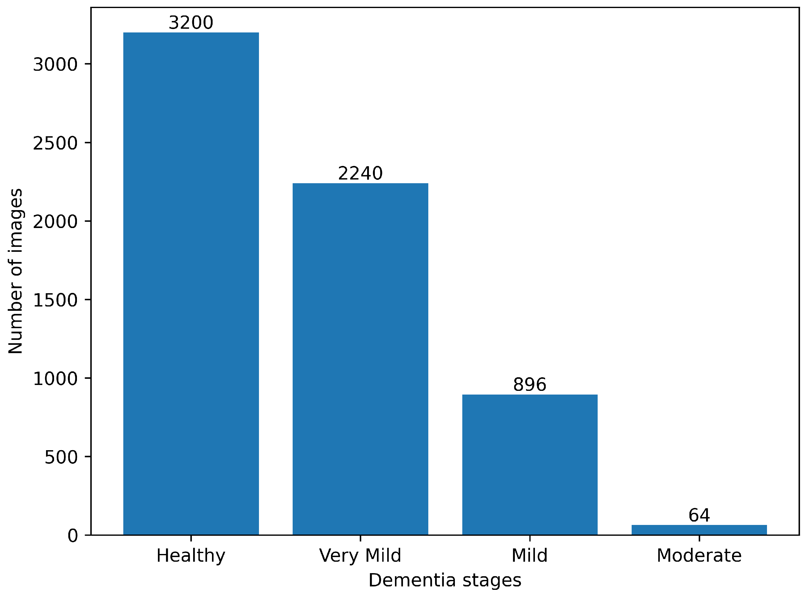
4.1. Data Description
4.2. Preprocessing
4.3. Network Implementation
4.4. Evaluation Metrics
5. Discussion
6. Conclusions
Author Contributions
Funding
Institutional Review Board Statement
Informed Consent Statement
Data Availability Statement
Acknowledgments
Conflicts of Interest
References
- WHO. Dementia; WHO: Geneva, Switzerland, 2023. [Google Scholar]
- Javeed, A.; Dallora, A.; Berglund, J.; Ali, A.; Ali, L.; Anderberg, P. Machine Learning for Dementia Prediction: A Systematic Review and Future Research Directions. J. Med. Syst. 2023, 47, 17. [Google Scholar] [CrossRef] [PubMed]
- NIH. What Is Dementia; NIH: Bethesda, MD, USA, 2022. [Google Scholar]
- Alzheimer’s Society. What Is the Difference between Dementia and Alzheimer’s Disease? Alzheimer’s Society: London, UK, 2023. [Google Scholar]
- NIH. Mild Cognitive Impairment; NIH: Bethesda, MD, USA, 2022. [Google Scholar]
- NIH. Mild Cognitive Impairment; NIH: Bethesda, MD, USA, 2021. [Google Scholar]
- NIH. What Is Alzheimers; NIH: Bethesda, MD, USA, 2021. [Google Scholar]
- Krizhevsky, A.; Sutskever, I.; Hinton, G. Imagenet classification with deep convolutional neural networks. In Proceedings of the Advances in Neural Information Processing Systems, Lake Tahoe, NV, USA, 3–6 December 2012; Volume 25. [Google Scholar]
- Lim, B.Y.; Lai, K.W.; Haiskin, K.; Kulathilake, K.; Ong, Z.C.; Hum, Y.C.; Dhanalakshmi, S.; Wu, X.; Zuo, X. Deep learning model for prediction of progressive mild cognitive impairment to Alzheimer’s disease using structural MRI. Front. Aging Neurosci. 2022, 14, 560. [Google Scholar] [CrossRef] [PubMed]
- Basaia, S.; Agosta, F.; Wagner, L.; Canu, E.; Magnani, G.; Santangelo, R.; Filippi, M.; Alzheimer’s Disease Neuroimaging Initiative. Automated classification of Alzheimer’s disease and mild cognitive impairment using a single MRI and deep neural networks. Neuroimage Clin. 2019, 21, 101645. [Google Scholar] [CrossRef] [PubMed]
- Jiang, J.; Kang, L.; Huang, J.; Zhang, T. Deep learning based mild cognitive impairment diagnosis using structure MR images. Neurosci. Lett. 2020, 730, 134971. [Google Scholar] [CrossRef] [PubMed]
- Aderghal, K.; Afdel, K.; Benois-Pineau, J.; Catheline, G. Improving Alzheimer’s stage categorization with Convolutional Neural Network using transfer learning and different magnetic resonance imaging modalities. Heliyon 2020, 6, e05652. [Google Scholar] [CrossRef] [PubMed]
- Basheera, S.; Ram, M.S.S. A novel CNN based Alzheimer’s disease classification using hybrid enhanced ICA segmented gray matter of MRI. Comput. Med Imaging Graph. 2020, 81, 101713. [Google Scholar] [CrossRef] [PubMed]
- Acharya, U.R.; Fernandes, S.L.; WeiKoh, J.E.; Ciaccio, E.J.; Fabell, M.K.M.; Tanik, U.J.; Rajinikanth, V.; Yeong, C.H. Automated detection of Alzheimer’s disease using brain MRI images—A study with various feature extraction techniques. J. Med. Syst. 2019, 43, 1–14. [Google Scholar] [CrossRef] [PubMed]
- Nagarathna, C.; Kusuma, M.; Seemanthini, K. Classifying the stages of Alzheimer’s disease by using multi layer feed forward neural network. Procedia Comput. Sci. 2023, 218, 1845–1856. [Google Scholar]
- Kapadnis, M.N.; Bhattacharyya, A.; Subasi, A. Artificial intelligence based Alzheimer’s disease detection using deep feature extraction. In Applications of Artificial Intelligence in Medical Imaging; Elsevier: Amsterdam, The Netherlands, 2023; pp. 333–355. [Google Scholar]
- Wee, C.Y.; Liu, C.; Lee, A.; Poh, J.S.; Ji, H.; Qiu, A.; Alzheimers Disease Neuroimage Initiative. Cortical graph neural network for AD and MCI diagnosis and transfer learning across populations. Neuroimage Clin. 2019, 23, 101929. [Google Scholar] [CrossRef] [PubMed]
- Guo, J.; Qiu, W.; Li, X.; Zhao, X.; Guo, N.; Li, Q. Predicting Alzheimer’s disease by hierarchical graph convolution from positron emission tomography imaging. In Proceedings of the 2019 IEEE International Conference on Big Data (Big Data), Los Angeles, CA, USA, 9–12 December 2019; IEEE: Piscataway, NJ, USA, 2019; pp. 5359–5363. [Google Scholar]
- Park, S.; Yeo, N.; Kim, Y.; Byeon, G.; Jang, J. Deep learning application for the classification of Alzheimer’s disease using 18F-flortaucipir (AV-1451) tau positron emission tomography. Sci. Rep. 2023, 13, 8096. [Google Scholar] [CrossRef] [PubMed]
- Tajammal, T.; Khurshid, S.; Jaleel, A.; Wahla, S.Q.; Ziar, R.A. Deep Learning-Based Ensembling Technique to Classify Alzheimer’s Disease Stages Using Functional MRI. J. Healthc. Eng. 2023, 2023, 6961346. [Google Scholar] [CrossRef] [PubMed]
- Liu, S.; Masurkar, A.; Rusinek, H.; Chen, J.; Zhang, B.; Zhu, W.; Fernandez-Granda, C.; Razavian, N. Generalizable deep learning model for early Alzheimer’s disease detection from structural MRIs. Sci. Rep. 2022, 12, 17106. [Google Scholar] [CrossRef] [PubMed]
- O’Malley, T.; Bursztein, E.; Long, J.; Chollet, F.; Jin, H.; Invernizzi, L. KerasTuner. 2019. Available online: https://github.com/keras-team/keras-tuner (accessed on 1 August 2023).
- Simonyan, K.; Zisserman, A. Very deep convolutional networks for large-scale image recognition. arXiv 2014, arXiv:1409.1556. [Google Scholar]
- Hong, D.; Gao, L.; Yao, J.; Zhang, B.; Plaza, A.; Chanussot, J. Graph convolutional networks for hyperspectral image classification. IEEE Trans. Geosci. Remote. Sens. 2020, 59, 5966–5978. [Google Scholar] [CrossRef]
- Selvaraju, R.; Cogswell, M.; Das, A.; Vedantam, R.; Parikh, D.; Batra, D. Grad-cam: Visual explanations from deep networks via gradient-based localization. In Proceedings of the IEEE International Conference On Computer Vision, Venice, Italy, 22–29 October 2017; pp. 618–626. [Google Scholar]
- Duchi, J.; Hazan, E.; Singer, Y. Adaptive subgradient methods for online learning and stochastic optimization. J. Mach. Learn. Res. 2011, 12, 2121–2159. [Google Scholar]
- Ioffe, S.; Szegedy, C. Batch normalization: Accelerating deep network training by reducing internal covariate shift. In Proceedings of the International Conference on Machine Learning, PMLR, Lille, France, 6–11 July 2015; pp. 448–456. [Google Scholar]
- Kumar, N. ADNI-Extracted-Axial. 2021. Available online: https://www.kaggle.com/ds/1830702 (accessed on 10 August 2023).
- Gupta, Y.; Lama, R.K.; Kwon, G.R.; Initiative, A.D.N. Prediction and classification of Alzheimer’s disease based on combined features from apolipoprotein-E genotype, cerebrospinal fluid, MR, and FDG-PET imaging biomarkers. Front. Comput. Neurosci. 2019, 13, 72. [Google Scholar] [CrossRef] [PubMed]
- Payan, A.; Montana, G. Predicting Alzheimer’s disease: A neuroimaging study with 3D convolutional neural networks. arXiv 2015, arXiv:1502.02506. [Google Scholar]
- Khvostikov, A.; Aderghal, K.; Benois-Pineau, J.; Krylov, A.; Catheline, G. 3D CNN-based classification using sMRI and MD-DTI images for Alzheimer disease studies. arXiv 2018, arXiv:1801.05968. [Google Scholar]
- Valliani, A.; Soni, A. Deep residual nets for improved Alzheimer’s diagnosis. In Proceedings of the 8th ACM International Conference on Bioinformatics, Computational Biology, and Health Informatics, Boston, MA, USA, 20–23 August 2017; p. 615. [Google Scholar]
- Helaly, H.; Badawy, M.; Haikal, A. Deep learning approach for early detection of Alzheimer’s disease. Cogn. Comput. 2021, 14, 1711–1727. [Google Scholar] [CrossRef] [PubMed]


| Class | n (Classified) | n (Truth) | F1 Score | Recall | Precision |
|---|---|---|---|---|---|
| Healthy | 853 | 645 | 0.59 | 0.69 | 0.52 |
| Very Mild | 223 | 452 | 0.30 | 0.22 | 0.45 |
| Mild | 152 | 173 | 0.10 | 0.09 | 0.11 |
| Moderate | 52 | 10 | 0 | 0 | 0 |
| Class | n (Classified) | n (Truth) | F1 Score | Recall | Precision |
|---|---|---|---|---|---|
| Healthy | 553 | 667 | 0.83 | 0.76 | 0.91 |
| Very Mild | 701 | 429 | 0.68 | 0.87 | 0.55 |
| Mild | 26 | 171 | 0.23 | 0.13 | 0.88 |
| Moderate | 0 | 13 | 0 | 0 | 0 |
| Class | n (Classified) | n (Truth) | F1 Score | Recall | Precision |
|---|---|---|---|---|---|
| Healthy | 640 | 640 | 1 | 1 | 1 |
| Very Mild | 460 | 448 | 0.99 | 1 | 0.97 |
| Mild | 180 | 180 | 1 | 1 | 1 |
| Moderate | 0 | 12 | 0 | 0 | 0 |
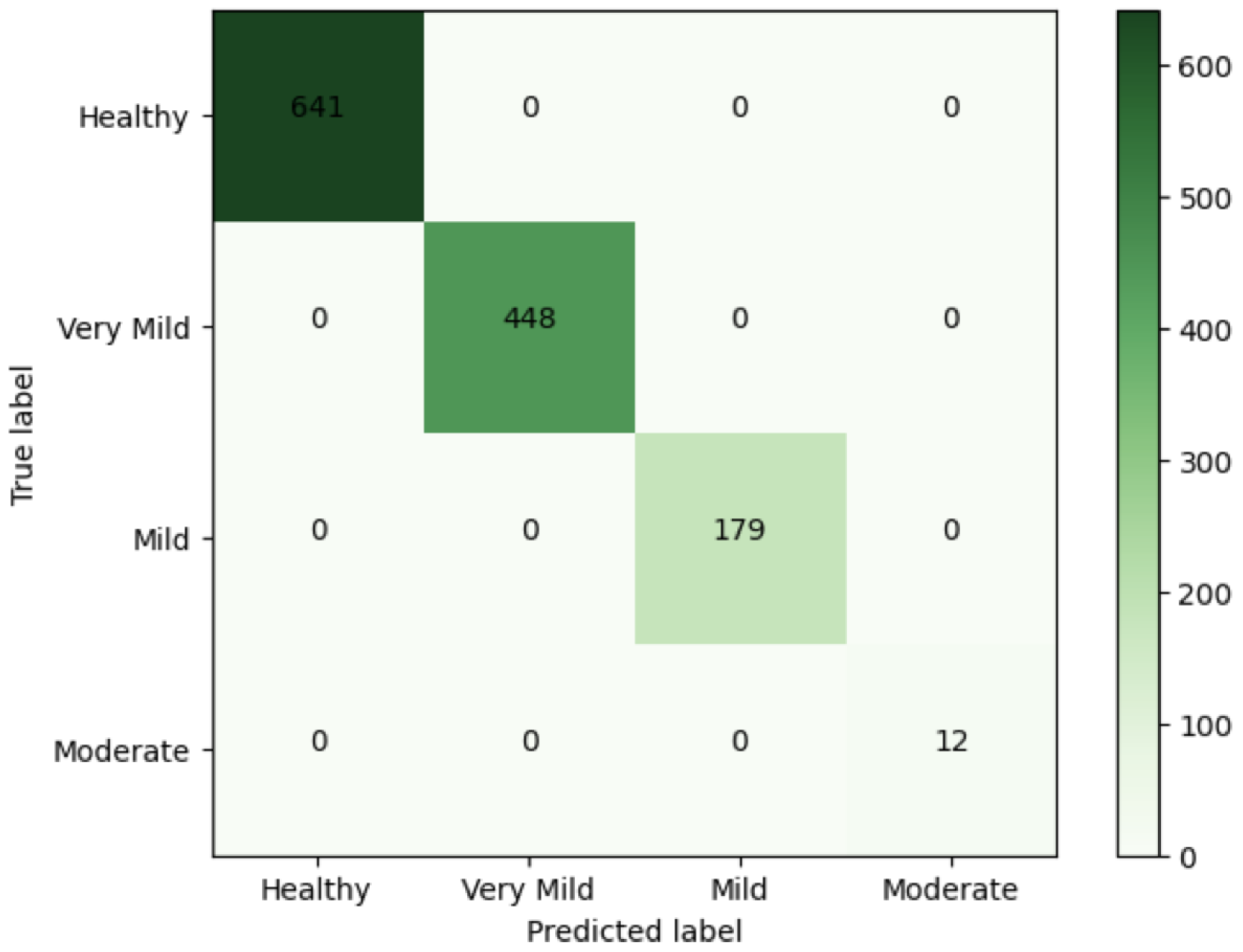
| Class | n (Classified) | n (Truth) | F1 Score | Precision | Recall |
|---|---|---|---|---|---|
| Healthy | 641 | 641 | 1 | 1 | 1 |
| Very Mild | 448 | 448 | 1 | 1 | 1 |
| Mild | 179 | 179 | 1 | 1 | 1 |
| Moderate | 12 | 12 | 1 | 1 | 1 |
| Paper | No. of Classes | CNNs | Pre-Trained VGG | GCNs | CNN-GCN | ResNet-50 | VGG16-SVM |
|---|---|---|---|---|---|---|---|
| Our work | Multi-class (4 way) | 43.83% | 71.17% | 99.06% | 100% | 59.69% | |
| Lim et al. [9] | Multi-class (3 way: CN vs. MCI vs. AD) | 72.70% | 78.57% | 75.71% | |||
| Jiang et al. [11] | Binary (EMCI vs. NC) | 89.4% | |||||
| Payan et al. [30] | Binary (AD vs. HC, MCI vs. HC, AD vs. MCI) | 95.39%, 92.13%, 86.84% | |||||
| Khvostikov et al. [31] | Binary (AD vs. HC, MCI vs. HC, AD vs. MCI) | 93.3%, 73.3%, 86.7% | |||||
| Valliani et al. [32] | Multi-class (3 way: AD vs. MCI vs. CN) | 49.2% | 50.8% | ||||
| Helaly et al. [33] | Multi-class (4 way: AD vs. EMCI vs. LMCI vs. NC) | 93% |
| Model | CNNs | VGG16 with Additional Convolutional Layers | GCNs | CNN-GCN |
|---|---|---|---|---|
| GPU time (s) | 411 | 2364 | 64 | 95 |
Disclaimer/Publisher’s Note: The statements, opinions and data contained in all publications are solely those of the individual author(s) and contributor(s) and not of MDPI and/or the editor(s). MDPI and/or the editor(s) disclaim responsibility for any injury to people or property resulting from any ideas, methods, instructions or products referred to in the content. |
© 2024 by the authors. Licensee MDPI, Basel, Switzerland. This article is an open access article distributed under the terms and conditions of the Creative Commons Attribution (CC BY) license (https://creativecommons.org/licenses/by/4.0/).
Share and Cite
Hasan, M.E.; Wagler, A. New Convolutional Neural Network and Graph Convolutional Network-Based Architecture for AI Applications in Alzheimer’s Disease and Dementia-Stage Classification. AI 2024, 5, 342-363. https://doi.org/10.3390/ai5010017
Hasan ME, Wagler A. New Convolutional Neural Network and Graph Convolutional Network-Based Architecture for AI Applications in Alzheimer’s Disease and Dementia-Stage Classification. AI. 2024; 5(1):342-363. https://doi.org/10.3390/ai5010017
Chicago/Turabian StyleHasan, Md Easin, and Amy Wagler. 2024. "New Convolutional Neural Network and Graph Convolutional Network-Based Architecture for AI Applications in Alzheimer’s Disease and Dementia-Stage Classification" AI 5, no. 1: 342-363. https://doi.org/10.3390/ai5010017
APA StyleHasan, M. E., & Wagler, A. (2024). New Convolutional Neural Network and Graph Convolutional Network-Based Architecture for AI Applications in Alzheimer’s Disease and Dementia-Stage Classification. AI, 5(1), 342-363. https://doi.org/10.3390/ai5010017