Abstract
Accidents due to defective railway lines and derailments are common disasters that are observed frequently in Southeast Asian countries. It is imperative to run proper diagnosis over the detection of such faults to prevent such accidents. However, manual detection of such faults periodically can be both time-consuming and costly. In this paper, we have proposed a Deep Learning (DL)-based algorithm for automatic fault detection in railway tracks, which we termed an Ensembled Convolutional Autoencoder ResNet-based Recurrent Neural Network (ECARRNet). We compared its output with existing DL techniques in the form of several pre-trained DL models to investigate railway tracks and determine whether they are defective or not while considering commonly prevalent faults such as—defects in rails and fasteners. Moreover, we manually collected the images from different railway tracks situated in Bangladesh and made our dataset. After comparing our proposed model with the existing models, we found that our proposed architecture has produced the highest accuracy among all the previously existing state-of-the-art (SOTA) architecture, with an accuracy of 93.28% on the full dataset. Additionally, we split our dataset into two parts having two different types of faults, which are fasteners and rails. We ran the models on those two separate datasets, obtaining accuracies of 98.59% and 92.06% on rail and fastener, respectively. Model explainability techniques like Grad-CAM and LIME were used to validate the result of the models, where our proposed model ECARRNet was seen to correctly classify and detect the regions of faulty railways effectively compared to the previously existing transfer learning models.
1. Introduction
Since 1862, the railway has been an integral element of Southeast Asia as a cost-effective, safe, and convenient mode of transportation for all classes of people. Railway tracks have played a crucial part in carrying masses over them in the form of passenger trains and good transportation trains. But train accidents can inflict huge damage to a nation as their aftermath brings a much more horrifying scenario compared to any other transportation accident.
The majority of the accidents occur due to derailments that have gruesomely stacked up many deaths. According to [1] 43% of all subsequent train accidents and 67 percent of the death toll in India are caused by railroad level crossings. The fatality rate from different countries might show different numbers but one thing that remains constant is its high percentage. In [2], a comparative analysis of accidents was performed in Bangladesh during 2008–2014, where among 18,771 accidents, (12%) took place on railways. A lot of effort was put into accident prevention and recovery but less work is being conducted on railway accident prevention in Bangladesh [3]. Identifying the faults present on railway tracks and attending to their repairs can prevent accidents. However, the fault detection method is done manually in Bangladesh railways. Manual detection and analysis of faults are hectic, which can also cause a lack of accuracy if people are assigned to cover the huge distances of railway tracks for inspection. This is because they can easily miss some damaged spots which may cause accidents. Additionally, people with good technical knowledge of railway tracks and their subsequent components like fasteners, sleepers, and railway switchers need to inspect the tracks. Here, DL techniques can come in handy as they can replace any manual detection techniques which are laborious, time-consuming, and inefficient. As a result, this will lead to faster and more rapid crisis response thus leading to less number of accidents and death.
DL has effectively proved its capability for image processing for quite a while. One of its huge triumphs was accomplished when transfer learning architectures like -Alexnet [4] exhibited their adequacy for the massive scale of image processing tasks. After that, we witnessed the development of a few remarkable Neural Network (NN) models, such as VGG16 [5] as well as exceptional results for image recognition in everyday applications, including medical image analysis [6,7,8] for the detection of lung diseases and the investigation of ransom calls, face recognition [9,10], object detection with imagery from unmanned aerial vehicles [11,12] and much more.
Automatic detection of such faults using DL can cause the process to be much more convenient and produce more accurate results. To elaborate, different models like InceptionV3, InceptionResnetV2, Xception, etc have been applied to different datasets, we have observed these existing algorithms and their corresponding research papers along with their produced results and have introduced our version of the model that has produced better accuracy. We have tried to look into the possible limitations in their papers and analyzed what blunders we can avoid to strengthen our model. For our research work, we have collected our data, which is primary data, from different cities of Bangladesh like-Satkhira and Feni and trained the images with our customized algorithm-ECARRNet and we also have added model explainability. The following are the significant contributions of this work:
- The dataset which we have collected consists of a total of 428 images from both faulty and non-faulty railway tracks from two different parts of the track, i.e., from rails and fasteners. Since it is hard to find faulty images, we have augmented our dataset to increase in size before training, and class imbalance problems were also fixed using oversampling techniques like SMOTE.
- Three SOTA CNN-based transfer learning models (InceptionV3, InceptionResnetV2, and Xception) have been used to classify and detect the faults on railway tracks, and their respective performances are presented using several metrics such as accuracy curves, confusion matrices, and classification reports.
- An ensembled DL architecture, ECARRNet has been proposed, to predict defective (faulty) and non-defective (non-faulty) railway tracks with greater predictive performance than existing SOTA.
- Explainable AI tools in the form of Grad-CAM and LIME are used to explore the black-box nature of the models and further validate our results to prove the efficacy of our proposed model.
The remaining component of the paper is assembled as follows: Section 2 presents background data on the algorithm used by earlier researchers working on railway identification of defects as well as a selection of well-written research publications on our topic of study. The details of data acquiring, pre-processing, breakdown of dataset construction, and the architecture of proposed and compared models are all described in Section 3. Section 4 conveys the results section, which features visualizations of the observations in terms of the accuracies and losses of each model, while the conclusion is discussed in Section 5.
2. Related Works
We have found various ML, DL, and computer vision-based approaches to detect railway track faults autonomously while doing our background study. Authors of [13] proposed a model where they used multiple models and got different results from them. They have proposed DL models in the form of Inception V3, ResNet50, and Faster R-CNN to detect faults in Loose Ballast, SunKink, Track Switch, and Signals. They ran these models on more than 100 GB of video data and got 96% accuracy for Loose Ballast, 100% accuracy SunKink, 95.6% accuracy for Track Switch, and 99.4% for Signal Color models. Also, they prepared a track health index using those data. Lin, Y. et al. [14] have suggested a GPS-based method that determines the fault’s location and uses a GO pro camera to take photographs. YOLO v3 has been used as an updated model of YOLO in their proposed architecture, which has a base network with darknet-53. Moreover, they have used Feature Prediction Network (FPN) to upgrade the ability of prediction for small objects. They have captured the images of fasteners and emphasized on detection of fasteners. Thus, they have shown the precision to be 89% and the recall being 95%.
In paper [15], the authors have proposed a multiphase DL technique to perform the segmentation of images. First, they detected the track surface defect using visual-based track inspection systems (VTIS) and located the Regions of Interest (ROI). The segmentation usually works by cropping the segmented image on the ROI. They have demanded their accuracy increase from 71% to 90% as shown in Table 1. In this study [16], the U-net graph segmentation network and the saliency cues approach of damage location were used to identify high-speed rail damage. Their detection accuracy rate is 99.76%.
Researchers at paper [17], have discovered that combining image processing and feeding that data into a neural network (NN) is more effective and efficient than alternative approaches. They have used the backpropagation method and talked about a hidden layer that will be trained using a dataset created and absolute output, with 1 denoting railway track cracks and 0 denoting no cracks. On the other hand, paper [18] has proposed conventional image processing to detect defects in fasteners and to remove noise from the image which includes techniques like a median filter, binary image conversion, Gaussian noise removal, etc. along with a projection algorithm. The use of Dense-SIFT features was suggested as a strategy for fault detection and identification. Finally, VGG16 was trained to recognize and diagnose fastener defects. Furthermore, Faster RCNN was also applied to increase the detection rate and efficiency. They have shown an accuracy of 97.14% using the Faster VGG16 network.
Min, Y. et al. [19] used scar and crackle in real-time using machine vision techniques to detect defects. This paper proposed a damage detection model where the image is collected at first using a plane array camera along with LED light to increase the brightness of the picture. Then the target area is localized to extract value from H in Hue, Saturation, and Lightness (HSL). After that, the authors used several image enhancement techniques to get more features from the image such as—image denoising, threshold value, and morphological processing. They also extracted the contour information of the faulty location using directional chain code tracking methods. M. Karakose and colleagues in [20] have devised a technique for detecting railway faults using two separate units. They created IAS to fulfill three tasks: expanding train tracks, enhancing contrast, and automating the defect detection procedure. They transformed the image to grayscale first, then utilized three separate Canny Edge Detection techniques.
In this work [21], the authors have offered an automated video analysis-based rail track inspection approach. They kept track of how many edge pixels each window has. The density of edges in each window is determined by this. The peak value was calculated by charting edge density in each window vs. window numbers. The clip’s location is represented by this peak. When the peak value is less than a certain threshold, the window is regarded to contain noise rather than a clip. The frame will be tagged as containing two clips if two peak values are both greater than a defined threshold. As a result, they achieve an average accuracy of 95.3%. In research [22], they have proposed an entirely CNN-based system, trained on ten different classes of materials, then feature-mapped using ten different channels. Their purpose was to concurrently identify the most likely fastener position inside each preset ROI and then categorize those detections into one of three fundamental conditions: background (or absent fastener), broken fastener, or good fastener. They tested our fastener detector on 85 kilometers of continuous trackbed photos to see how accurate it is. Using the Deep CNN MLT 3 Method, they were able to attain 95.02% accuracy.
Alawad, H. et al. [23] present a monitoring technique that makes use of computer vision to automatically and quickly detect hazards in stations by recognizing risky acts, giving real-time support for decision-makers, and minimizing the possible effects of undesirable events. Then they build a sequential model at each layer, which is the simplest form of a layer in the Keras library. With their CNN-0 model, they were able to attain an accuracy of 81.90%. Kamilaris, A. et al. [24] compared strategies for the same data in the same research paper, using the same measure. The prominent CNN architectures including AlexNet, VGG, and Inception-ResNet were used. They also experimented with their designs, some of which combined CNN with other approaches.
Yang, C. et al. [25] have proposed an ML-based railway inspection approaches, which include a feature-based technique and a deep neural network-based technique based on acceleration data. As a result, ResNet and FCN are examined in this work. Three convolution blocks are used to construct FCN, which is then succeeded by a soft-max layer and a global average pooling layer. By establishing a shortcut link between consecutive convolutional layers, ResNet expands neural networks to a very deep structure. The results of the experiments showed that ResNet and fully convolutional networks (FCN) both performed well in joint detection. Yao, H. et al. [26] have suggested a model in which the RNN is seen as having a similar ability to Convolutional Neural Network to derive features from pictures. CNN and RNN are of equal importance. To better balance the two types of characteristics recovered by the CNN and RNN during the training phase, the model uses the perceptron attention mechanism to weigh the features received by the CNN and RNN, respectively. They used stackable LSTM as the RNN module to extract the time sequence properties from the pixels. The CNN (Inception-ResNet V2) technique was also utilized, and the greatest accuracy was 83%.
Evaluation Metrics used in DL tasks have a critical role in generating the best classifier, according to Alzubaidi, L. et al. [27], they are used in two steps of a typical data categorization procedure: training and testing. They discussed FPGA, which can be used to create CNN overlay engines with over 80% efficiency, eight-bit precision, and over 15 TOPs peak performance. Voxnet’s accuracy was 79%, whereas ResNet’s was 80%. In the framework of the European Common Agricultural Policy, CamposTaberner, M. et al. [28] want to learn more about an RNN for land use categorization based on Sentinel-2 time series (CAP). The results of the investigation show that the red and near-infrared Sentinel-2 bands provide the most helpful data. The traits acquired from summer acquisitions were the most important in terms of temporal information. The performance precision of the 2-BiLSTM network in every class is over 91.4%.
Shafique, R. et al. [29] provide an acoustic analysis-based autonomous railway track defect detection system. The data collected on Pakistani railway lines using acoustic signals and the application of various classification systems to the gathered data are two major contributions of this work. They achieve the greatest outcomes with RF and DT, which have a 97% accuracy rate. A DL-based fault diagnosis network for RVSFD was built by Ye, Y. et al. [30]. There are three phases to the diagnostic network: The GWN strategy is used to the acceleration signal in the first phase (data preprocessing) to make the diagnostic network resistant to relatively high-frequency influences induced by track imperfections. An EST strategy is presented in the second step (training dataset creation) to increase the diagnostic network’s robustness against wheel wear. Finally, a GONEST-1D CNN-based fault diagnosis network of high-speed train suspension systems is created in the third phase (training and recognition). All the states can be completely recognized using the confusion matrix given for the testing samples (100%).

Table 1.
Overview of the Reviewed Sources.
Table 1.
Overview of the Reviewed Sources.
| Ref. | Task | Datasets | Classifiers | Accuracy |
|---|---|---|---|---|
| [13] | Proposed models to detect faults in Loose Ballast, SunKink, Track Switch, and Signals. | Datasets are made from the 100 GB of video data | Inception V3, ResNet50, and Faster R-CNN | 100% |
| [14] | GPS determines the fault’s location and use a GO pro camera to take photographs. | Datasets are made from the images extracted from video data | Yolo v3 | 95% |
| [15] | Proposed a multiphase DL technique to perform segmentation of images. | Datasets are made from the actual rail tracks that are collected by a COTS VTIS. | Visual-based track inspection systems(VTIS), TrackNet | 90% |
| [16] | To detect high-speed railway rail damage, a combination of the U-net graph segmentation network and the saliency cues approach of damage localization was presented. | Type-I RSDDs dataset | SCueU-Net | 99.76% |
| [18] | They proposed defect detection and identification methods using Dense-SIFT features. | Dataset is made up of images that are taken from Beijing Metro Line 6. | RCNN, VGG16 | 97.14% |
| [19] | Proposes a damage detection model where the Image is collected at first using a plane array camera along with LED light to increase the brightness of the picture. | Datasets are made from the images of plane array camera | Directional chain code tracking | .... |
| [20] | A computer-based visual rail condition monitoring is proposed. | Data acquired from a camera placed on top of the train | Image processing | .... |
| [21] | An automated video analysis based rail-track inspection approach. | Data acquired from a video camera placed in front of the train | Image processing | 95.3% |
| [22] | Automated track inspection using computer vision and pattern recognition methods. | Data acquired from a camera placed in front of the moving train | Deep CNN | 95.02% |
| [23] | Using computer vision and pattern recognition, perform risk management in railway systems. | Manually collected images from different rail tracks | Keras, ReLU, CNN | 81.90% |
| [24] | Eexamines the research questions related to agriculture, the models used, the data sources used, and the overall precision attained based on the authors’ performance indicators. | PlantVillage, LifeCLEF, MalayaKew and UC Merced | AlexNet, VGG, and Inception-ResNet | .... |
| [25] | Proposed machine learning-based railway inspection approaches, including a feature-based method and a deep neural network-based method based on acceleration data. | The acceleration dataset was obtained from the sensors mounted to the rail inspection car. | ResNet, FCN | 100% |
| [27] | Provide a more comprehensive survey of the most important aspects of DL and, including those enhancements recently added to the feld. | ImageNet, CIFAR-10, CIFAR-100, MNIST | Xillinx, Voxnet, ResNet | 80% |
| [28] | Shows the use of DL approaches for the analysis of remote sensing (RS) data is rapidly increasing. | Datasets are built from remote sensing (RS) data and satellite data | Sentinel-2, 2-BiLSTM, CamposTaberner | 91.4% |
| [29] | Provide an acoustic analysis-based autonomous railway track defect detection system. | Datasets are built from the data collected on Pakistani railway lines using acoustic signals | Vector machines, LR, RF, and DT | 97% |
| [30] | A DL-based fault diagnosis network for RVSFD was built. | Datasets are built from the data collected from accelerometer sensors. | GONEST-1D CNN | 100% |
3. Methodology
3.1. Overview of the Proposed Architecture
We are proposing a new Ensembled Convolutional Autoencoder Resnet-based Recurrent neural Network-based deep architecture (ECARRNet) for railway fault detection and compared our results with conventional models to show the prospect of RNN-based models in image classification as shown in Figure 1. Moreover, there are some major advantages of using a CNN-RNN ensembled model which also outperforms conventional CNN models. Firstly, we are using convolutional autoencoders to reduce the dimensionality of images and to extract important features from the data. In the next stage, our proposed model contains a resnet-based transfer learning architecture trained on the imagenet dataset so that we can use the useful network weights in our model to solve the problem of lack of enough data, which can reduce our performance. Thirdly, we are also using an LSTM layer which has memory cells instead of just recurrent units, to store and output information with the help of gating mechanisms and thus extend the capability of RNN. Lastly, we are using a few layers of fully connected neural network layers before our final binary classification layer. We are also giving special attention to reducing vanishing or exploding gradient problems, as our proposed architecture is quite deep. We are making use of initialization parameters such as He kernel initializer to initialize weights, which would play a key role in reducing vanishing or exploding gradients. In addition, batch normalization layers are also contributing to reducing vanishing gradient problems and also act as a regularization parameter. The proposed model is described in detail below in Table 2 that gives an overview of the model in terms of its layers and their types.
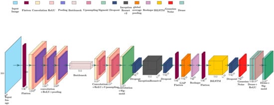
Figure 1.
Architecture of the Proposed Model.
Table 2.
Model architecture summary.
3.1.1. Convolutional Autoencoder
Auto-encoder is an unsupervised neural network model which produces output data with less noise and distortion. It is commonly used in data compression tasks and also reduces the storage space of data, improves the training time, and discards variables that are redundant. On the other hand, the convolutional neural network is also great for extracting useful features from images. So, we are using convolutional layers to improve the performance of a simple auto-encoder. We have also experimented with only a convolutional neural network in the first stage of our model and found that the convolutional auto-encoder gives better performance. Simple Autoencoders mainly have 3 parts—an encoder, code, and decoder. At first, the input passes the encoder to produce the code, where the encoder is a fully connected neural network. Then, the decoder produces an output only using the code, where the decoder is also a fully connected artificial neural network. The objective of this step is to get an output that is identical to the input. The decoder architecture often gives a mirror image of the encoder. In an auto-encoder, the dimensionality of the input and output should always be the same.
Convolutional auto-encoder adds specialty to the basic structure of a simple auto-encoder by replacing the fully connected layers in the encoder and decoder portion with convolutional layers. The size of the input layers will also be equal to the size of the output layers, similar to a simple auto-encoder. The decoder network in the convolutional auto-encoder also transforms itself into transposed convolutional layers. Along with convolutional layers, max-pooling layers are also included as well in the encoder and decoder network. Convolutional auto-encoders have many use cases, such as—image compression, image denoising, etc. [31,32]. In our proposed architecture, we have experimented with different encoder and decoder architectures to find the optimal architecture. Our encoder architecture has 3 convolutional layers and 3 max-pooling layers, and the layers are further strengthened with the use of batch normalization and dropout layers. The first convolutional layer has 128 neurons with a 6 × 6 filter size and ReLU as the activation function. We are also using a special kernel initializer called normalization to reduce the vanishing gradient. All the max-pooling layers consist of a pooling size of 2. In the next two convolutional layers, we are using 2D convolutional layers with 64 neurons, each with a 4 × 4 filter size. In the decoder portion, the first 2D convolutional layer has 64 neurons, and also it has several 2D up-sampling layers with a filter size of 2 × 2 to reconstruct the same output dimension as input. The next convolutional layer has 128 neurons, and the last one has only one neuron with a sigmoid activation function. All the convolutional layers in the decoder have a filter size of 6 × 6.
In the convolutional auto-encoder part and our overall proposed model, we have used batch normalization layers frequently and almost in between every layer. This is because, in the beginning, our training was really slow as the data set and the model was relatively big and was prone to overfitting. After using batch normalization extensively, our training time improved significantly and due to the regularization effect of the batch normalization, it played a key role in producing state-of-the-art accuracy. According to [33], while training a deep neural network, the distribution of each layer’s input changes during training as the parameters of the previous layers change. As a result, training slows down and needs lower learning rates and much more careful parameter initialization. Thus, it becomes difficult to train models with saturating nonlinearities which are known as internal covariate shifts. To solve this problem, we can normalize layer inputs for each training mini-batch, as it allows the usage of higher learning rates by getting less careful about initialization. Batch normalization is capable of achieving the same accuracy with 14 times fewer training steps and significantly beats the model which did not use batch normalization at all.
3.1.2. Resnet Based Transfer Learning
In this stage, we are using a resnet-based transfer learning architecture which is trained on the imagenet dataset. In transfer learning, we apply the expertise acquired by a model from a task with abundant training data to improve performance on a new task with limited data availability. In our problem, since we did not have so much initial data, so we had to take the help of transfer learning to leverage what they have already learned in one task to enhance the ability to generalize in another context. Therefore, we are using a pre-trained model known as inception-ResNet-v2 which performed better than other pre-trained networks such as—inceptionv3, Xception, etc. in our dataset. Inception architecture has already been proven through many research works to give good performance at a low cost comparatively. Moreover, it was found that training with residual inception networks speeds up the training of inception networks largely. Residual connections in resnet consist of convolutional layers along with relu activation functions. In Inception-ResNet, batch normalization is used only on top of the traditional layers, but not on top of the summarizations [34].
3.1.3. Recurrent Neural Network
This stage explains the unique portion of our proposed model. In this part, we use recurrent neural networks, which is an artificial neural networks in which connections between individual units form a directed cycle. RNN can model the dynamical behavior of sequences with arbitrary lengths. In our proposed architecture, along with the convolutional layers in the Inception-ResNet-v2 described above, it thus creates a combined CNN-RNN framework as the data reaches the RNN layer after passing the CNN layers. The CNN-RNN framework for image classification has many benefits [35]. In general, the recurrent neural network is more suitable for modeling sequential data. In the CNN-RNN model, RNN generates sequential predictions for various timesteps using the output of CNN as input. Image data is often considered two-dimensional wave data in which convolution layers act as a filtering process. Convolutional layers are able to filter simple band information in an image but often leave behind important features of image information. Therefore, using an RNN layer is important because the CNN-RNN framework can make use of RNN to calculate the dependency and continuity features of the intermediate layer output of the CNN model. It also allows the connection of the characteristics of these middle tiers to the full connection network for classification prediction, which thus leads to a better classification accuracy [36].
However, because the gradient must pass through numerous layers of the RNN, it creates long-term dependency and thus frequently experiences vanishing and exploding gradient issues, making it challenging to model. To solve this problem, we are using Long-Short Term Memory (LSTM) in our proposed model. LSTM consists of memory cells to encrypt knowledge at each instant of time. Three gates—an input gate, a forget gate, and an output gate—control how the memory cell behaves. To be more precise, memory cells of LSTM form a cell state which passes relevant information from earlier time steps to later time steps, thereby, reducing the effect of short-term memory. As the cell state carries information throughout the sequence, information is added or removed by the gates. Gates are independent neural networks for deciding which information should be allowed or discarded from the cell state. On the other hand, gates consist of sigmoid activation functions. They give output values between 0 and 1 when passed through them. This principle is used by different gates. Forget gate makes decisions about which information should be kept or discarded. As the information from the previous hidden state crosses the current input, it passes through the sigmoid function. The sigmoid function produces a value between 0 and 1, if the value is closer to 0, it is forgotten and if it is close to 1 then it has to be remembered by the cell state. Input gates are used to update the cell state. Finally, output gates are used which decide which hidden state to use. Therefore, these gates assist the input signal to pass through the recurrent hidden states by retaining useful information in the long run and removing unnecessary redundant information. In this way, LSTM is well capable of solving the vanishing and exploding gradient problem and can model long-term term temporal dynamics pretty well, which RNN cannot. In our paper, we are using a bidirectional LSTM layer with 2900 neurons which helps in forming the CNN-RNN architecture which has several advantages as mentioned above. We have also experimented with another gated version of RNN called GRU, but bidirectional LSTM with 2900 neurons performed better in our dataset.
3.1.4. Fully Connected Layers
Lastly, our ensemble deep network consists of some fully connected layers as well. After the LSTM layer, we add 2 more dense or fully connected layers consisting of 100 neurons each. Finally, We have some dropout regularizers, along with batch normalization layers before our last layer. The last layer is a dense layer with a sigmoid function for binary classification.
Lastly, we want to briefly discuss some essential parts to demonstrate the unique feature of our proposed model, which allows us to produce such good performance. We are using a batch size relatively low due to a lack of computational resources, typically less than 10. Dimensions of images used are typically 300 by 300, but our experimentation shows 500 by 500 and often 600 by 600 images produce the best result. We are using Adamax optimizer as it is able to better optimize than Adam. We used binary cross entropy as our loss function.
3.2. Comparison Models Overview
We have used 3 different state-of-the-art models for image classification in our research to evaluate our dataset and compare the obtained results with our proposed model. The briefings of the comparison models in terms of their architectures are discussed below.
3.2.1. InceptionV3
A model made by researchers at Google, which is a modified version of the inception architecture [37]. Despite the model consisting of 42 layers, the computational cost is only times greater than GoogleNet. In image classification in ILSVRC, it has become the 1st runners-up which proves its efficacy. The Inception V3 model was trained with the dataset used in this research and we determined its accuracy in both training and validation.
3.2.2. Xception
Depthwise Separable Convolutions are used in the deep CNN architecture known as “Xception”. In Inception, the original input is compressed using 1 × 1 convolutions, and each depth space is then given a new set of filters based on the input spaces. Just the opposite occurs with Xception. Before compressing the input space using convolution by applying it across the depth, it first applies the filters to each of the depth maps. We used Xception as it does not introduce any non-linearity.
3.2.3. InceptionResNetV2
It is a deep convolutional neural network having 164 layers. Input images having dimensions of are fed into the model that is passed through a convolutional block with output dimensions of having a stride of 32 followed by another convolutional layer having the same dimensions and stride. The next layer has a stride of 64 that is fed into a convolutional layer and a maxpool layer. The resulting layer is passed through 2 consecutive layers of convolutional neural networks layers having dimensions of with a depth of 64 and with a depth of 96 respectively and through 4 layers of the convolutional layer having dimensions of with a depth of 64, with a depth of 64 with a depth of 64 and with a depth of 96. Both the emerging layers are passed through a filter concat and eventually, the resulting output layers are passed through a convolutional layer and a maxpool layer having strides of 2. Final output layers are passed through a filter concat.
4. Performance Evaluation Parameters
We are using accuracy as our performance metrics, and we are also testing the performance of our model using metrics like—classification reports and confusion matrices. Our classification report has four metrics to measure the effectiveness of each of the models. The metrics include Support, Precision, F1 score, and recall. Support can be calculated by summing the last rows in the confusion matrix. Support is the number of occurrences of each particular class in the true responses which means that it shows the number of actual occurrences of the class in the dataset.
In the above set of equations,
- TP = True Positive
- FP = False Positive
- FN = False Negative
- TN = True Negative
AI models are usually considered black-box models, and they lack transparency. Transparent models can explain why they predict and what they predict. It thus builds trust in the model and makes sure that they are predicting only the desired object in a way that is explainable to researchers. The objective of transparency is to find out cases in which the model has failed substantially. There are several approaches and frameworks available to implement explainable AI, which can produce visual demonstrations to provide a better understanding of what a model predicts on new samples of data and how they do it. In the case of images, patches are produced to indicate the location on which the model is focusing. One of the most popular approaches to providing LIME (Local Interpretable Model-Agnostic Explanations) is a revolutionary explanation method to faithfully and comprehensibly explain the predictions of any classifier. We are using LIME in our paper to explain the performance of our proposed model as we could not find any other available solution to explain our custom model. Additionally, we are using Grad-CAM which produces heat-maps on the location of the image where the model is focusing [38]. We are using Grad-CAM to obtain the model explainability of the models, which are used to compare with our proposed architecture. LIME is an algorithm that can faithfully explain the predictions of any classifier and regressor by localizing it with an understandable model [39].
The results produced by both Grad-CAM and LIME are shown in the experimental results section.
Equation (4) shows the equation of Grad-CAM which is a weighted linear combination of feature maps followed by a ReLU function. Where,
- = feature map activation
- = neuron significance weight
5. Experimental Results
5.1. Data Collection
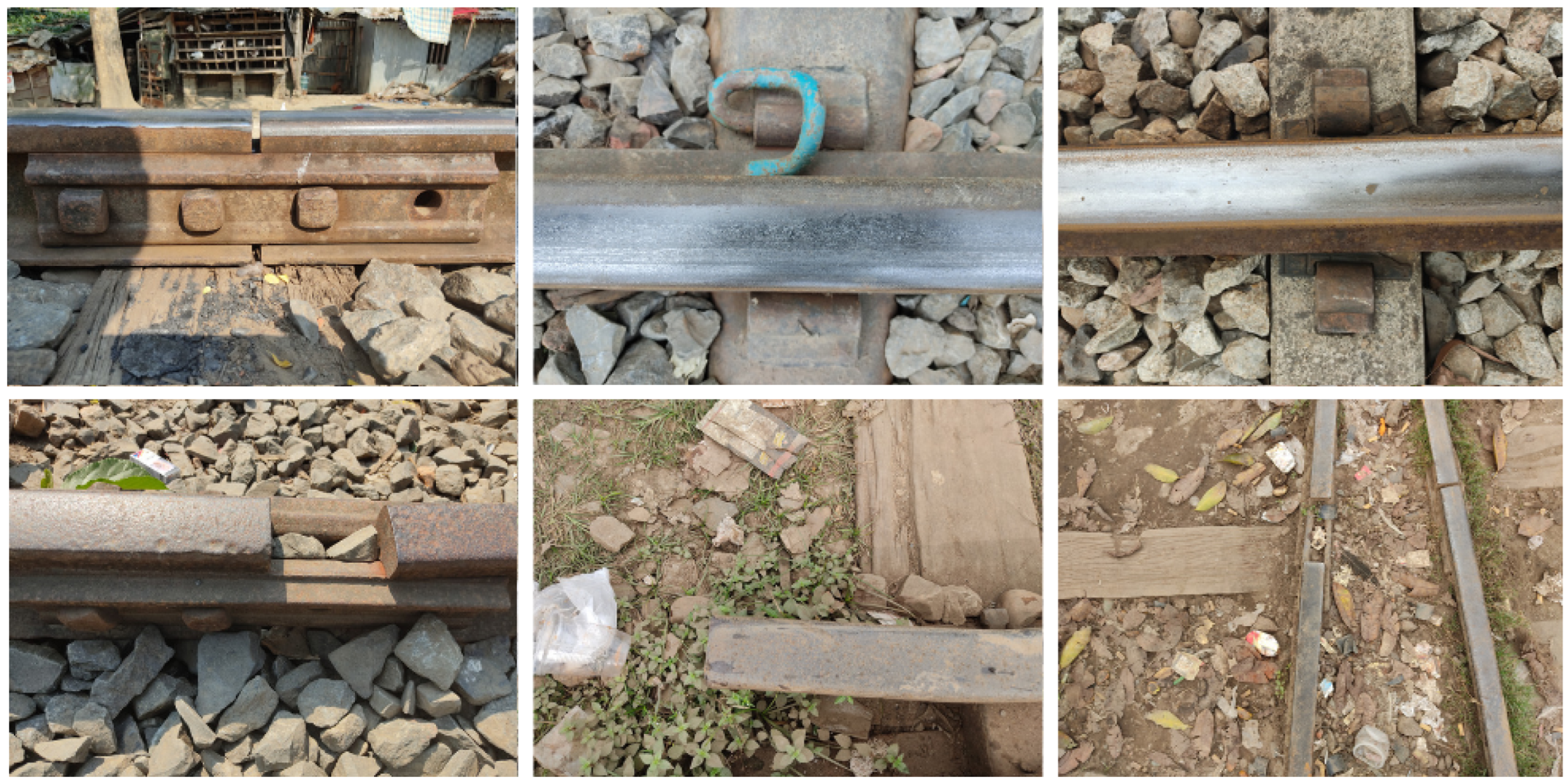
We have collected our dataset by visiting railway tracks in different locations across Bangladesh [40]. Since the railway tracks were constructed many years earlier, only faults for meter gauge and broad gauge lines were found. We went to the railway tracks at Jessore and Feni and took photographs from different places in the city for several days. We went to stations and junctions collecting data from old, new, and abandoned rail tracks. We have also considered abandoned tracks because we can not find all kinds of faults in regular tracks. We have mainly found faults in rails and fasteners, which are one of the major components of railway tracks and are usually responsible for causing drastic accidents. To make a statistically significant dataset, we could only use faults of sleepers and fasteners images for training our model. We have collected 428 images in total, containing 156 defective and 272 non-defective images. We tried to take images from different angles for each type of error. Some of the sample images of our initial dataset are shown in Figure 2

Figure 2.
Samples of faults on railway tracks.
5.2. Data Pre-Processing
At first, we prepared 3 different versions of the dataset to train and experiment to find which way of arranging data would work best. In the 1st version, we used only images of rails that contained defective and non-defective classes of images from faults in rails. In the 2nd version, we have defective and non-defective images from fasteners [41] only and in the last and final version, we have defective and non-defective images from both rails and fasteners combined. This makes our experiment and proposed model more reliable, as it is repeated multiple times in multiple scenarios to produce similar results. We also cropped each image according to the region of interest and prepared our dataset by dividing them into test, train, and validation, each containing different types of fault.
We have done four types of augmentation and thus the number of images increased to four times from the initial number, i.e., up to 1712 images. Moreover, we have also used the ImageDataGenerator class from Keras for in-code augmentation to mutliply the number of images in our dataset. In-code augmentation using TensorFlow and Keras increases the size of the dataset during the training process without occupying any physical memory. We used rotation, vertical flip, horizontal flip, brightness, etc. as parameters. Altogether, we have used around 8000 images for training.
On the other hand, we have also faced a class imbalance problem, as we could not find faulty images in adequate numbers on railway tracks. As a result, we found more images of railway tracks that are non-defective or with no faults. Therefore, we had to apply an oversampling technique called SMOTE (Synthetic Minority Oversampling Technique), which is a very successful technique for class imbalance problems. SMOTE creates copies of the images for the class that is a minority or has less number of images. SMOTE does this by producing data points on the same lines, which connects a point and one of its KNNs [42].
Finally, we would also like to mention that we have used shuffling methods such as—stratified K-fold shuffle splits to ensure that both of our classes are in equal quantity in train and test splits. This ensures that our data is not randomly sampled in train, validation, and test splits. As a result, this makes our experiments more valid by reducing sampling bias and increasing the validity of our experiments.
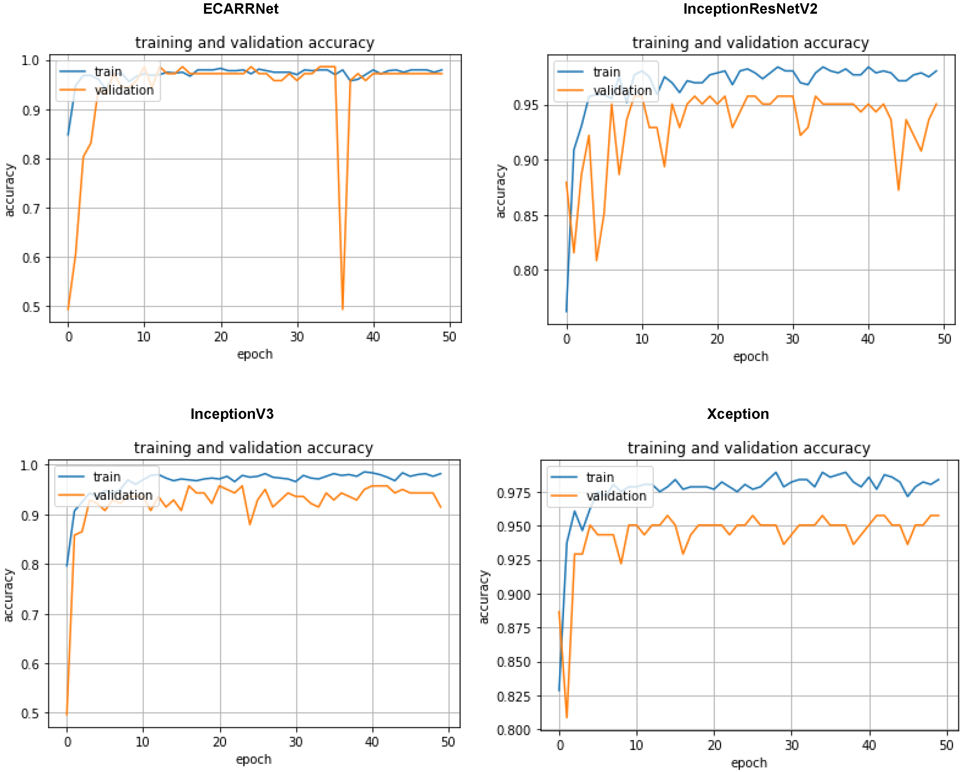
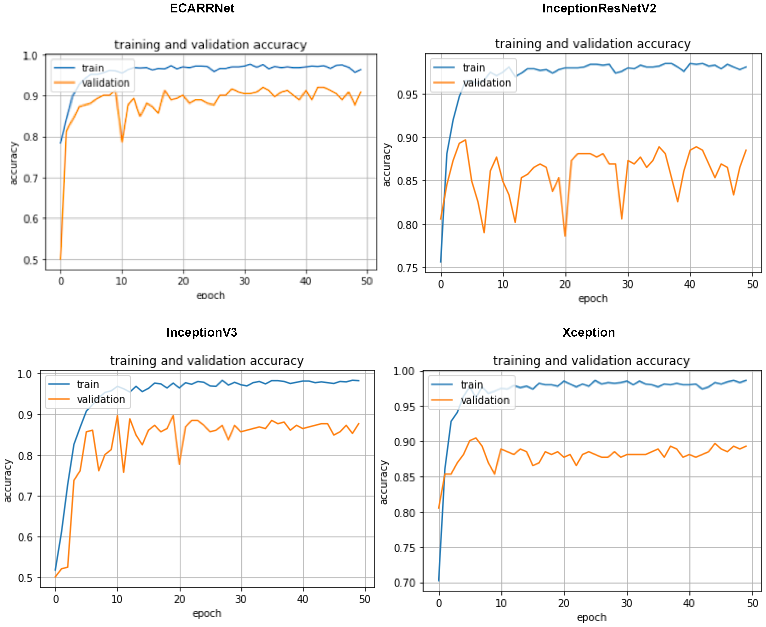
5.3. Results Generated on Rail Dataset
Figure 3 displays the set of accuracy curves for the implemented algorithms. The curves indicate that our proposed model ECARRNet outperforms the other models in terms of peak accuracy and average accuracy.
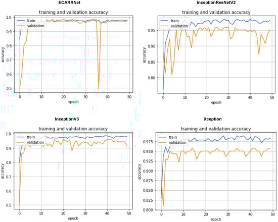
Figure 3.
Accuracy curves for each of the models on the rail dataset.
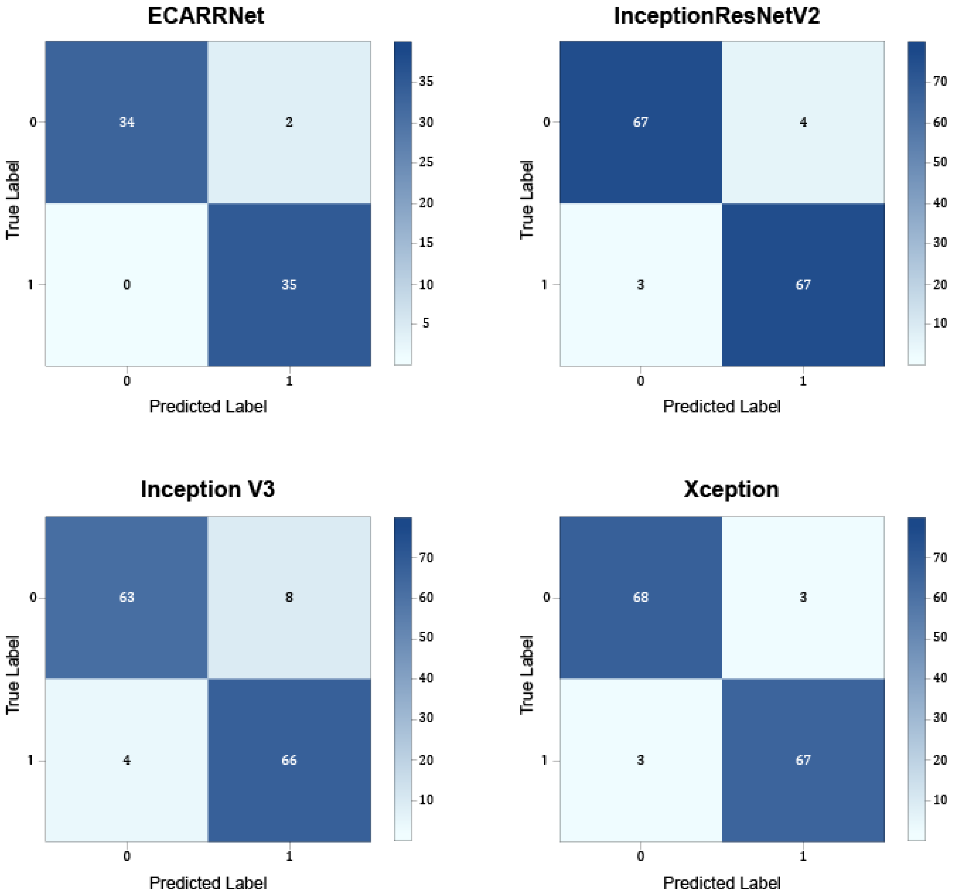
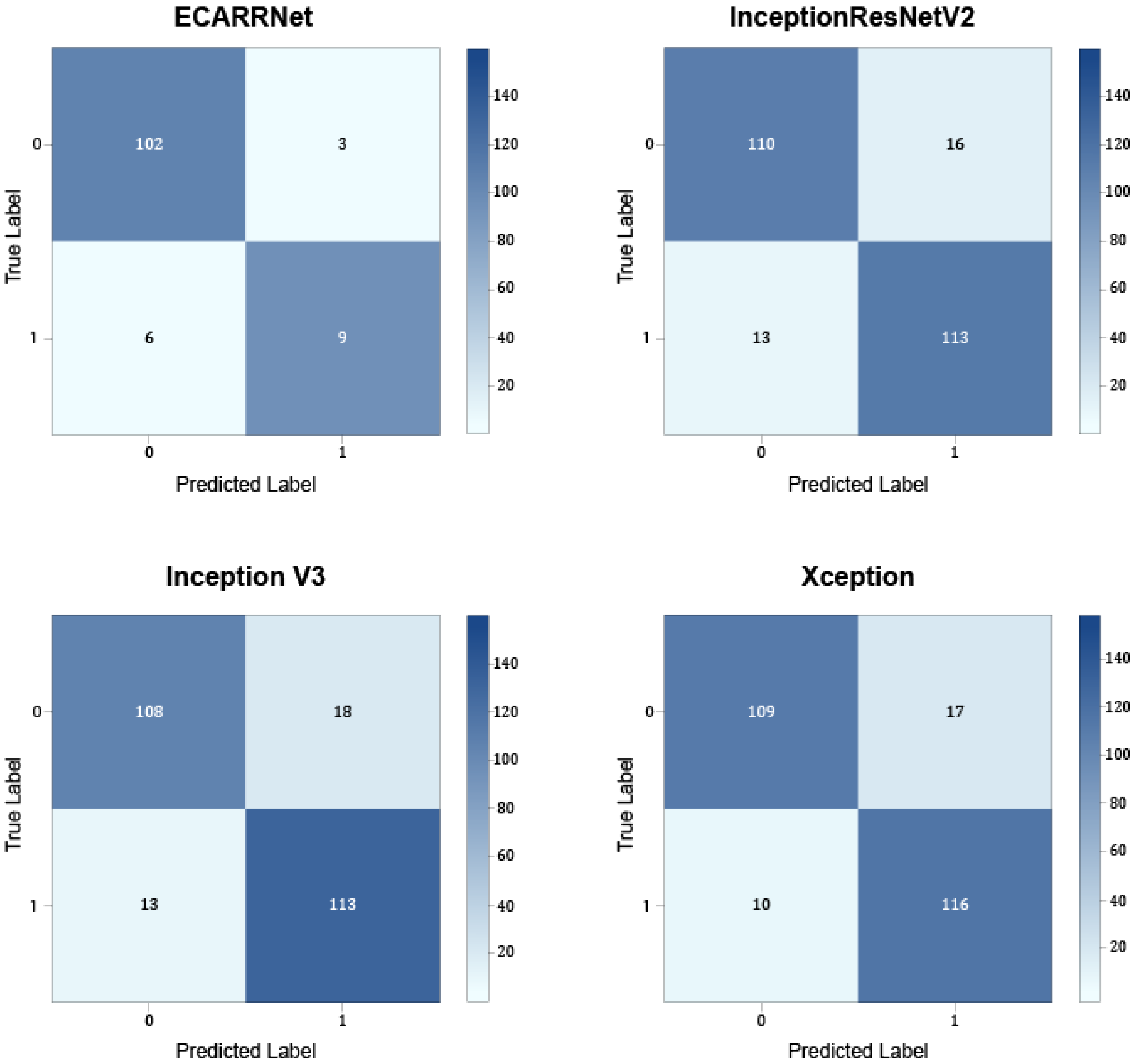
Figure 4 exhibits the confusion matrices for the models on the rail dataset. The results show that ECARRNet produces less false positives compared to InceptionV3 and produces similar and comparative results when compared to InceptionResnetV2 and Xception respectively.

Figure 4.
Confusion matrices for each of the models on the rail dataset.
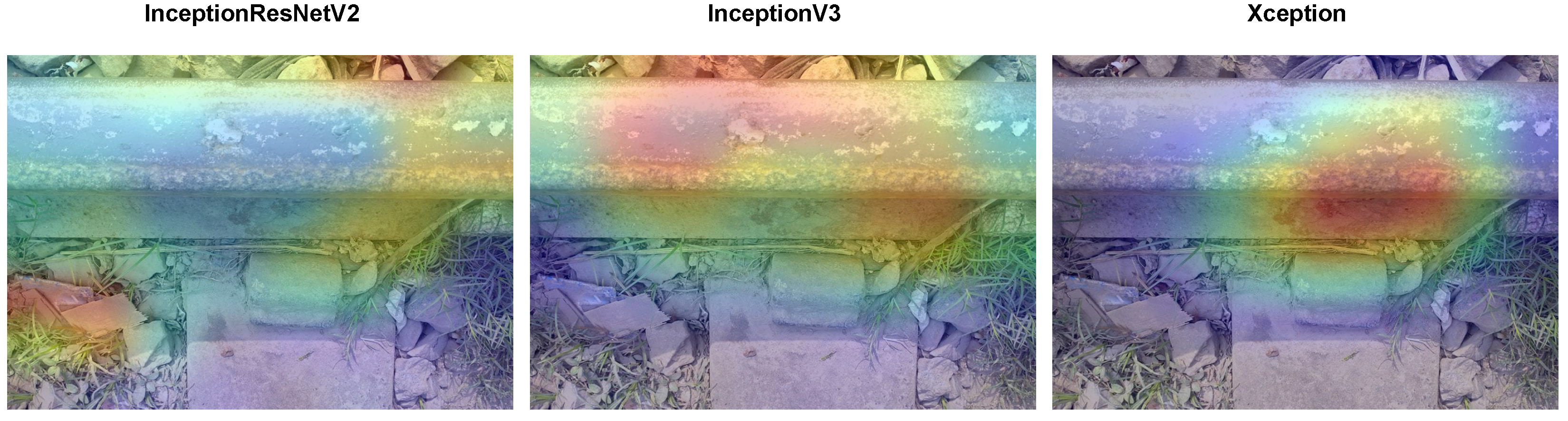
Figure 5 portrays the Grad-CAM visualizations for the same image selected randomly from the rail dataset for the compared models. The region of the heatmap generated using the InceptionResnetV2 model classifies the incorrect region in the image where there is no fault, as the red region which represents the highest contribution of the model for classification is not in the defective portion of the track. InceptionV3 and Xception, on the other hand, produce heatmaps that comparatively fall much closer to the region of faulty rail tracks.
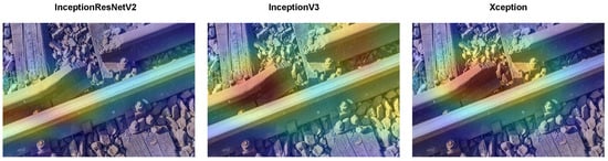
Figure 5.
Grad-CAM visualizations for transfer learning models on rail dataset.
From Table 3, we can see Xception performs better than the other models when compared on the RAIL dataset. It has the best F1 score () for both defective and non-defective classes, as well as the maximum precision and recall (). With equal F1 scores of , InceptionResnetV2 and ECARRNet exhibit very competitive performance, lagging Xception by a small margin. Even though it is still a powerful model, InceptionV3 performs somewhat worse than the others, with the lowest F1 score of . All things considered, Xception is the top model for this particular dataset, exhibiting the best balance in accurately classifying defective and non-defective cases.
Table 3.
Classification Report for Rail Dataset.
5.4. Results Generated on Fastener Dataset
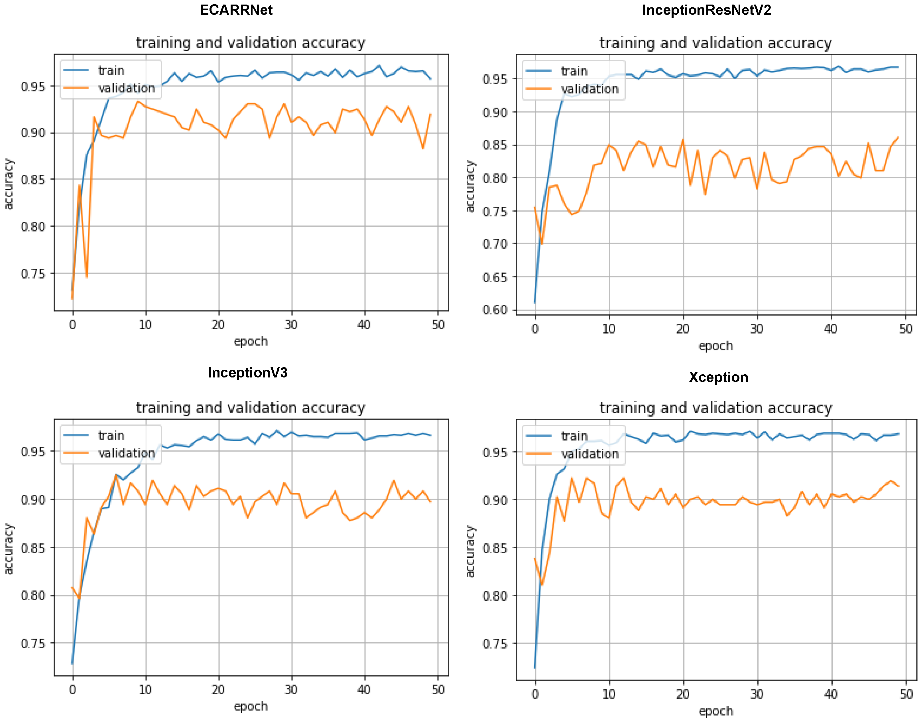
In Figure 6 the accuracy curves of the models based on the fastener dataset are displayed. Once again we see our ECARRNet model outperforming the other transfer learning models. InceptionV3 and Xception produce results that are comparable to ECARRNet while InceptionResNetV2 performs very poorly on the fastener dataset.
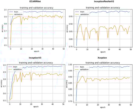
Figure 6.
Accuracy curves for each of the models on fastener dataset.
Figure 7 exhibits the confusion matrices for the models on the fastener dataset. The results show that ECARRNet produces fewer false positives compared to InceptionV3 and produces similar and comparative results when compared to InceptionResnetV2 and Xception respectively.
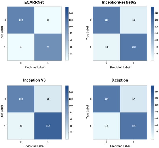
Figure 7.
Confusion matrices for each of the models on fastener dataset.
Figure 8 portrays the Grad-CAM visualizations for the same image selected randomly from the fastener dataset for the compared models. The region of the heatmap generated using the InceptionResnetV2, InceptionV3, and Xception models produces heatmaps that classify a region that is somewhat close to the faulty fasteners on all images, but the red region which shows high contribution for classification is not exactly focusing on the fastener portion which is defective or faulty.
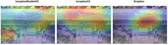
Figure 8.
Grad-CAM visualizations for transfer learning models on fastener dataset.
Table 4 with the highest F1 ratings of for both the defective and non-defective categories, Xception shines out once more and suggests a balanced precision and recall. With an F1 score of , InceptionV3 comes in second with a good recall and slightly less precision. With an F1 score of , InceptionResnetV2 and ECARRNet perform identically across all criteria. Overall, on this dataset, Xception performs similarly and consistently to the other models, with the exception of a minor edge in correctly categorizing defective and non-defective items.
Table 4.
Classification Report for Fastener Dataset.
5.5. Results Generated on Full Dataset
In Figure 9, the accuracy curves of the models based on the full dataset are displayed which includes defective and non-defective images from both fastener and rail. Once again, we see our ECARRNet model outperforming the other transfer learning models. InceptionV3 and Xception produce results that are comparable to ECARRNet while InceptionResNetV2 performs very poorly on the full dataset.
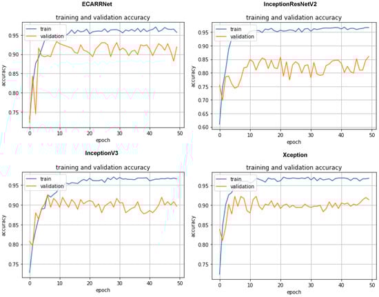
Figure 9.
Accuracy curves for each of the models on full dataset.
Figure 10 shows the confusion matrices for the models on the full dataset containing defective and non-defective images from both fastener and rail. The results show that ECARRNet produces fewer false positives compared to InceptionV3 and produces similar and comparative results when compared to InceptionResnetV2 and Xception respectively.
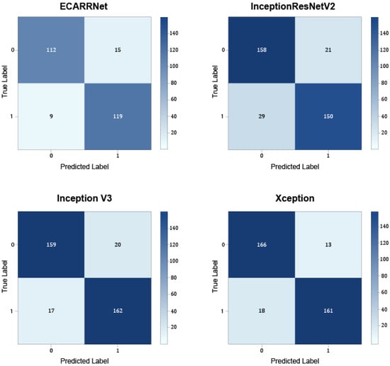
Figure 10.
Confusion matrices for each of the models on full dataset.
Figure 11 shows the Grad-CAM visualizations for the same image selected randomly from the full dataset which contains images of faults from both fastener and rail for the compared models. The region of the heatmap generated using the InceptionResnetV2, InceptionV3, and Xception models produces heatmaps that classify a region that is somewhat close to the faulty fasteners on all images, but the red region which shows high contribution for classification is not exactly focusing on the fault/gap portion in the rail which is defective or faulty.

Figure 11.
Grad-CAM visualizations for transfer learning models on full dataset.
In Table 5 with the best recall for non-defective items and the highest precision for defective items throughout the whole dataset, ECARRNet performs exceptionally well, earning an astounding F1 score of for both categories. Xception comes in second with an F1 score of , exhibiting balanced recall and precision in both areas. With an F1 score of , which is competitive but marginally lower than InceptionV3, the findings are strong. At for F1, InceptionResnetV2’s score is marginally lower than the others’. The macro and weighted averages agree with the F1 scores, indicating that ECARRNet is the best performing model in this assessment, followed closely by Xception and InceptionV3, and InceptionResnetV2 being the least successful of the four.
Table 5.
Classification Report for Full Dataset.
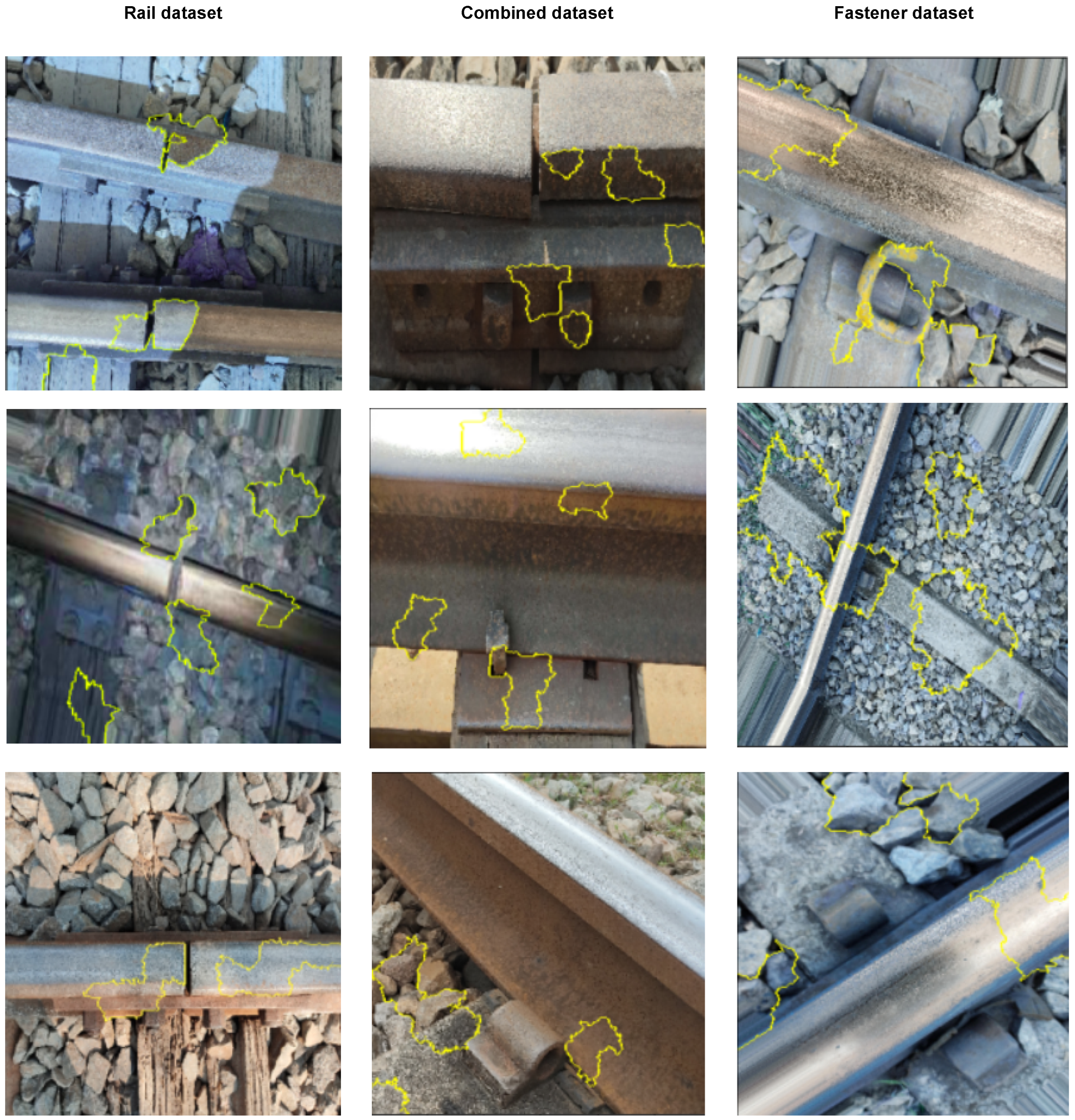
5.6. LIME Visualizations to Explain the Output Predictions of ECARRNet
Empirical analysis using GRADCAM shows that it works exceptionally well with transfer learning models like—InceptionResNetV2, InceptionV3, Xception, etc, but does not work for our proposed ensembled model which also consists of Bi-directional LSTM along with CNN models. GRADCAM was unable to handle our model and thus we could not obtain our desired visualization using GRADCAM. On the other hand, LIME is model-agnostic meaning, it can be used with any type of model. For this reason, we are using LIME to explain ECARRNet predictions. Figure 12 shows the visualizations for random images selected from the three different versions we have used for our experimentation purpose, i.e., the rail dataset, the combined dataset containing images of faults from both the rail and fastener and the fastener dataset using LIME visualizations. The generated visualizations which are wrapped in yellow boundaries are produced using only our proposed model, ECARRNeT. This region produced using LIME explains and shows the usefulness and robustness of our proposed model for detecting faults in railway tracks. It shows how accurately ECARRNet pinpoints the location of faults in railway tracks in all 3 versions of our dataset. It accurately wraps the faulty regions in rails and even pinpoints the faulty fasteners with utmost accuracy and very few false results. Therefore, these visualizations prove the supremacy of our ECARRNet model in predicting faults in railway tracks.
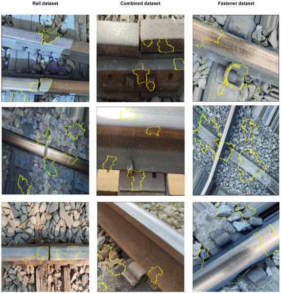
Figure 12.
LIME visualizations for ECARRNet model on each of the datasets.
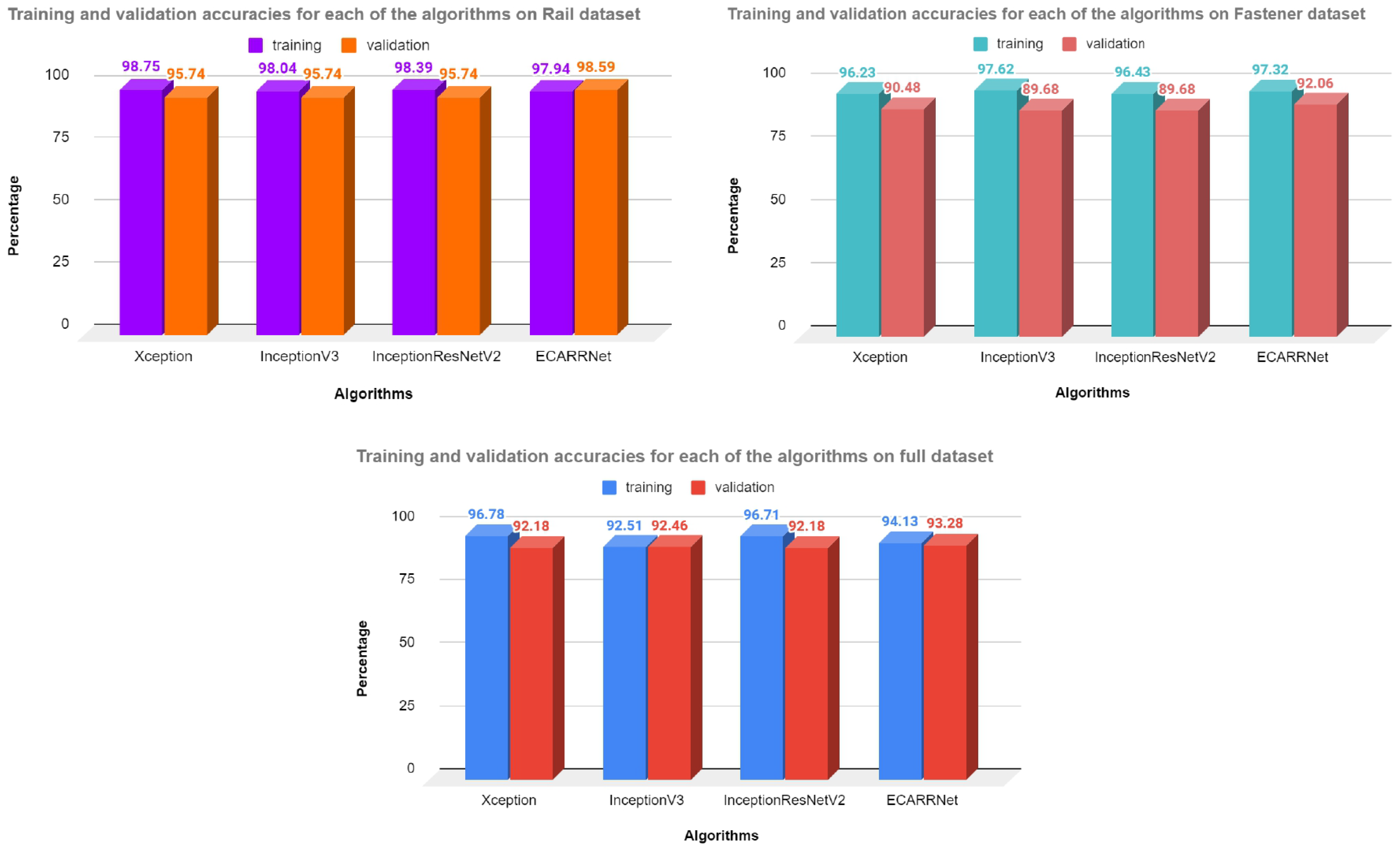
Figure 13 demonstrates the accuracy values in percentage for three different versions of the datasets. For each dataset, it compares the performance of our proposed model, ECARRNet with Xception, InceptionV3, and InceptionResNetV2, these models have also shown great results in image classification use cases. It also shows accuracy values for training and validation or test sets which clearly distinguishes the performances of ECARRNet from other models. We are considering the test or validation accuracy here for comparison because we have ensured that the test/validation set does not have any labels for each image. We have just provided the images to the models to predict the classes. Therefore we can see that validation accuracy is the highest for all 3 versions of the dataset for our proposed model ECARRNet, compared to other SOTA models for predicting faults in railway tracks. Also, by comparing results from Table 2, Table 3 and Table 4 we can also say that ECARRNet has shown expected results in other metrics like—precision, recall, F1 score, and in support as well. This means our proposed model is performing really well in predicting and distinguishing defective and non-defective railway tracks which once again proves its superiority against other popular CNN-based architectures for railway fault detection.

Figure 13.
Accuracy for each of the models on different datasets.
6. Conclusions
The main aim of this research paper is to distinguish between defective and fully functional railway tracks and to propose an automated solution to track faults to reduce accidents on railway track that leads to hundreds of deaths. We have carried out the classification and detection of railway faults by taking the aid of cutting-edge algorithms and our ensemble-based algorithm, ECARRNet. Our proposed model outperformed the other established algorithms and produced better results that was evident in the results obtained. In the future, we would like to collect more data from different parts of Bangladesh and other parts of the world to classify more categories of faults and improve on our proposed model.
Author Contributions
Conceptualization, S.I.E., S.H., A.A., A.E.M.R., M.S.I. and G.R.A.; methodology, S.I.E. and S.H.; software, S.I.E. and S.H.; validation, S.I.E. and S.H.; formal analysis, A.E.M.R., A.A., S.H. and S.I.E.; investigation, A.E.M.R. and A.A.; resources, S.I.E., S.H., A.A. and A.E.M.R.; data curation, A.E.M.R. and A.A.; writing—original draft preparation, A.A., S.H., S.I.E., A.E.M.R. and J.U.; writing—review and editing, A.A., S.H. and S.I.E.; visualization, S.H.; supervision, M.S.I., D.Z.K. and G.R.A.; project administration, M.S.I. and G.R.A.; funding acquisition, J.U. All authors have read and agreed to the published version of the manuscript.
Funding
This research is funded by Woosong University Academic Research 2024.
Institutional Review Board Statement
Not applicable for studies not involving humans.
Informed Consent Statement
Not applicable for studies not involving humans.
Data Availability Statement
The codes implemented in this paper using Tensorflow and Keras framework are available at—https://github.com/SalmanEunus27/ECARRNET---RAILWAY-FAULT-DETECTION-JOURNAL accessed on 25 March 2024.
Conflicts of Interest
The authors declare no conflict of interest.
References
- Singhal, V.; Jain, S.S.; Anand, D.; Singh, A.; Verma, S.; Kavita; Rodrigues, J.J.P.C.; Jhanjhi, N.Z.; Ghosh, U.; Jo, O.; et al. Artificial Intelligence Enabled Road Vehicle-Train Collision Risk Assessment Framework for Unmanned Railway Level Crossings. IEEE Access 2020, 8, 113790–113806. [Google Scholar] [CrossRef]
- Probha, N.A.; Hoque, M.S. A Study on transport safety perspectives in Bangladesh through comparative analysis of roadway, railway and waterway accidents. In Proceedings of the APCIM & ICTTE 2018: 2018 International Conference on Intelligent Medical & International Conference on Transportation and Traffic Engineering, Beijing, China, 21–23 December 2018; Association for Computing Machinery: New York, NY, USA, 2018; pp. 81–85. [Google Scholar] [CrossRef]
- Islam, M.M.; Ridwan, A.E.M.; Mary, M.M.; Siam, M.F.; Mumu, S.A.; Rana, S. Design and implementation of a smart bike accident detection system. In Proceedings of the 2020 IEEE Region 10 Symposium (TENSYMP), Dhaka, Bangladesh, 5–7 June 2020; pp. 386–389. [Google Scholar] [CrossRef]
- Krizhevsky, A.; Sutskever, I.; Hinton, G.E. ImageNet classification with deep convolutional neural networks. In Proceedings of the 25th International Conference on Neural Information Processing Systems, Lake Tahoe, NV, USA, 3–6 December 2012; NIPS’12. Curran Associates Inc.: Red Hook, NY, USA, 2012; Volume 1, pp. 1097–1105. [Google Scholar]
- Simonyan, K.; Zisserman, A. Very deep convolutional networks for large-scale image recognition. arXiv 2014, arXiv:1409.1556. [Google Scholar]
- Chen, H.; Zhang, Y.; Kalra, M.K.; Lin, F.; Chen, Y.; Liao, P.; Zhou, J.; Wang, G. Low-Dose CT With a Residual Encoder-Decoder Convolutional Neural Network. IEEE Trans. Med. Imaging 2017, 36, 2524–2535. [Google Scholar] [CrossRef] [PubMed]
- Anthimopoulos, M.; Christodoulidis, S.; Ebner, L.; Christe, A.; Mougiakakou, S. Lung Pattern Classification for Interstitial Lung Diseases Using a Deep Convolutional Neural Network. IEEE Trans. Med. Imaging 2016, 35, 1207–1216. [Google Scholar] [CrossRef] [PubMed]
- Rahman, R.; Rahman, M.A.; Hossain, S.; Hossain, S.; Akhond, M.R.; Hossain, M.I. RansomListener: Ransom Call Sound Investigation Using LSTM and CNN Architectures. In Proceedings of the 2021 6th International Conference on Inventive Computation Technologies (ICICT), Coimbatore, India, 20–22 January 2021; pp. 509–516. [Google Scholar] [CrossRef]
- Ding, C.; Tao, D. Robust Face Recognition via Multimodal Deep Face Representation. IEEE Trans. Multimed. 2015, 17, 2049–2058. [Google Scholar] [CrossRef]
- Sun, Y.; Chen, Y.; Wang, X.; Tang, X. Deep learning face representation by joint identification-verification. In Proceedings of the Advances in Neural Information Processing Systems; Ghahramani, Z., Welling, M., Cortes, C., Lawrence, N., Weinberger, K., Eds.; Curran Associates, Inc.: Red Hook, NY, USA, 2014; Volume 27. [Google Scholar]
- Chamoso, P.; Raveane, W.; Parra, V.; González, A. UAVs Applied to the Counting and Monitoring of Animals. In Ambient Intelligence—Software and Applications; Ramos, C., Novais, P., Nihan, C.E., Corchado Rodríguez, J.M., Eds.; Springer: Cham, Switzerland, 2014; pp. 71–80. [Google Scholar]
- Xu, Y.; Yu, G.; Wang, Y.; Wu, X.; Ma, Y. Car detection from low-altitude UAV imagery with the faster R-CNN. J. Adv. Transp. 2017, 2017, 2823617. [Google Scholar] [CrossRef]
- Mittal, S.; Rao, D. Vision Based Railway Track Monitoring using Deep Learning. arXiv 2017, arXiv:1711.06423. [Google Scholar]
- Lin, Y.W.; Hsieh, C.C.; Huang, W.H.; Hsieh, S.L.; Hung, W.H. Railway track fasteners fault detection using deep learning. In Proceedings of the 2019 IEEE Eurasia Conference on IOT, Communication and Engineering (ECICE), Yunlin, Taiwan, 3–6 October 2019; pp. 187–190. [Google Scholar] [CrossRef]
- James, A.; Jie, W.; Xulei, Y.; Chenghao, Y.; Ngan, N.B.; Yuxin, L.; Yi, S.; Chandrasekhar, V.; Zeng, Z. TrackNet—A deep learning based fault detection for railway track inspection. In Proceedings of the 2018 International Conference on Intelligent Rail Transportation (ICIRT), Singapore, 12–14 December 2018; pp. 1–5. [Google Scholar] [CrossRef]
- Lu, J.; Liang, B.; Lei, Q.; Li, X.; Liu, J.; Liu, J.; Xu, J.; Wang, W. SCueU-Net: Efficient Damage Detection Method for Railway Rail. IEEE Access 2020, 8, 125109–125120. [Google Scholar] [CrossRef]
- Welankiwar, A.; Sherekar, S.; Bhagat, A.P.; Khodke, P.A. Fault detection in railway tracks using artificial neural networks. In Proceedings of the 2018 International Conference on Research in Intelligent and Computing in Engineering (RICE), San Salvador, El Salvador, 22–24 August 2018; pp. 1–5. [Google Scholar] [CrossRef]
- Wei, X.; Yang, Z.; Liu, Y.; Wei, D.; Jia, L.; Li, Y. Railway track fastener defect detection based on image processing and deep learning techniques: A comparative study. Eng. Appl. Artif. Intell. 2019, 80, 66–81. [Google Scholar] [CrossRef]
- Min, Y.; Xiao, B.; Dang, J.; Yue, B.; Cheng, T. Real time detection system for rail surface defects based on machine vision. EURASIP J. Image Video Process. 2018, 3, 3. [Google Scholar] [CrossRef]
- Karakose, M.; Yaman, O.; Baygin, M.; Murat, K.; Akin, E. A New Computer Vision Based Method for Rail Track Detection and Fault Diagnosis in Railways. Int. J. Mech. Eng. Robot. Res. 2017, 6, 22–27. [Google Scholar] [CrossRef]
- Singh, M.; Singh, S.; Jaiswal, J.; Hempshall, J. Autonomous rail track inspection using vision based system. In Proceedings of the 2006 IEEE International Conference on Computational Intelligence for Homeland Security and Personal Safety, Alexandria, VA, USA, 16–17 October 2006; pp. 56–59. [Google Scholar] [CrossRef]
- Gibert, X.; Patel, V.M.; Chellappa, R. Deep Multitask Learning for Railway Track Inspection. IEEE Trans. Intell. Transp. Syst. 2017, 18, 153–164. [Google Scholar] [CrossRef]
- Alawad, H.; Kaewunruen, S.; An, M. A Deep Learning Approach Towards Railway Safety Risk Assessment. IEEE Access 2020, 8, 102811–102832. [Google Scholar] [CrossRef]
- Kamilaris, A.; Prenafeta-Boldú, F.X. A review of the use of convolutional neural networks in agriculture. J. Agric. Sci. 2018, 156, 312–322. [Google Scholar] [CrossRef]
- Yang, C.; Sun, Y.; Ladubec, C.; Liu, Y. Developing Machine Learning-Based Models for Railway Inspection. Appl. Sci. 2021, 11, 13. [Google Scholar] [CrossRef]
- Yao, H.; Zhang, X.; Zhou, X.; Liu, S. Parallel Structure Deep Neural Network Using CNN and RNN with an Attention Mechanism for Breast Cancer Histology Image Classification. Cancers 2019, 11, 1901. [Google Scholar] [CrossRef] [PubMed]
- Alzubaidi, L.; Zhang, J.; Humaidi, A.J.; Al-Dujaili, A.; Duan, Y.; Al-Shamma, O.; Santamaría, J.; Fadhel, M.A.; Al-Amidie, M.; Farhan, L. Review of deep learning: Concepts, CNN architectures, challenges, applications, future directions. Big Data 2021, 8, 53. [Google Scholar] [CrossRef] [PubMed]
- Campos-Taberner, M.; García-Haro, F.J.; Martínez, B.; Izquierdo-Verdiguier, E.; Atzberger, C.; Camps-Valls, G.; Gilabert, M.A. Understanding deep learning in land use classifcation based on Sentinel-2 time series. Sci. Rep. 2020, 10, 17188. [Google Scholar] [CrossRef]
- Shafique, R.; Siddiqui, H.U.R.; Rustam, F.; Ullah, S.; Siddique, M.A.; Lee, E.; Ashraf, I.; Dudley, S. A Novel Approach to Railway Track Faults Detection Using Acoustic Analysis. Sensors 2021, 21, 6221. [Google Scholar] [CrossRef]
- Ye, Y.; Huang, P.; Zhang, Y. Deep learning-based fault diagnostic network of high-speed train secondary suspension systems for immunity to track irregularities and wheel wear. Eng. Sci. 2021, 30, 96–116. [Google Scholar] [CrossRef]
- Chen, M.; Shi, X.; Zhang, Y.; Wu, D.; Guizani, M. Deep Feature Learning for Medical Image Analysis with Convolutional Autoencoder Neural Network. IEEE Trans. Big Data 2021, 7, 750–758. [Google Scholar] [CrossRef]
- Zhang, Y. A Better Autoencoder for Image: Convolutional Autoencoder. 2018. Available online: https://users.cecs.anu.edu.au/~Tom.Gedeon/conf/ABCs2018/paper/ABCs2018_paper_58.pdf (accessed on 25 March 2024).
- Ioffe, S.; Szegedy, C. Batch Normalization: Accelerating Deep Network Training by Reducing Internal Covariate Shift. CoRR 2015, arXiv:1502.03167. [Google Scholar]
- Szegedy, C.; Ioffe, S.; Vanhoucke, V. Inception-v4, Inception-ResNet and the Impact of Residual Connections on Learning. CoRR 2016, arXiv:1602.07261. [Google Scholar] [CrossRef]
- Guo, Y.; Liu, Y.; Bakker, E.; Guo, Y.; Lew, M. CNN-RNN: A large-scale hierarchical image classification framework. Multimed. Tools Appl. 2018, 77, 10251–10271. [Google Scholar] [CrossRef]
- Yin, Q.; Zhang, R.; Shao, X. CNN and RNN mixed model for image classification. MATEC Web Conf. 2019, 277, 02001. [Google Scholar] [CrossRef]
- Szegedy, C.; Vanhoucke, V.; Ioffe, S.; Shlens, J.; Wojna, Z. Rethinking the inception architecture for computer vision. In Proceedings of the IEEE Conference on Computer Vision and Pattern Recognition (CVPR), Boston, MA, USA, 7–12 June 2015. [Google Scholar] [CrossRef]
- Selvaraju, R.R.; Cogswell, M.; Das, A.; Vedantam, R.; Parikh, D.; Batra, D. Grad-CAM: Visual Explanations from Deep Networks via Gradient-Based Localization. Int. J. Comput. Vis. 2019, 128, 336–359. [Google Scholar] [CrossRef]
- Ribeiro, M.T.; Singh, S.; Guestrin, C. Why should I trust you?: Explaining the predictions of any classifier. In Proceedings of theKDD ’16: The 22nd ACM SIGKDD International Conference on Knowledge Discovery and Data Mining, San Francisco, CA, USA, 13–17 August 2016. [Google Scholar] [CrossRef]
- Adnan, A.; Hossain, S.; Shihab, R.; Ibne Eunus, S. Railway Track Fault Detection. 2021. Available online: https://www.kaggle.com/datasets/salmaneunus/railway-track-fault-detection (accessed on 25 March 2024).
- Adnan, A.; Hossain, S.; Shihab, R.; Ibne Eunus, S. Railway Track Fault Detection|Dataset 2 (Fastener) 2021. Available online: https://www.kaggle.com/datasets/ashikadnan/railway-track-fault-detection-dataset2fastener (accessed on 25 March 2024).
- Elreedy, D.; Atiya, A.F. A Comprehensive Analysis of Synthetic Minority Oversampling Technique (SMOTE) for handling class imbalance. Inf. Sci. 2019, 505, 32–64. [Google Scholar] [CrossRef]


Disclaimer/Publisher’s Note: The statements, opinions and data contained in all publications are solely those of the individual author(s) and contributor(s) and not of MDPI and/or the editor(s). MDPI and/or the editor(s) disclaim responsibility for any injury to people or property resulting from any ideas, methods, instructions or products referred to in the content. |
© 2024 by the authors. Licensee MDPI, Basel, Switzerland. This article is an open access article distributed under the terms and conditions of the Creative Commons Attribution (CC BY) license (https://creativecommons.org/licenses/by/4.0/).