Abstract
Software bug prediction is a software maintenance technique used to predict the occurrences of bugs in the early stages of the software development process. Early prediction of bugs can reduce the overall cost of software and increase its reliability. Machine learning approaches have recently offered several prediction methods to improve software quality. This paper empirically investigates eight well-known machine learning and deep learning algorithms for software bug prediction. We compare the created models using different evaluation metrics and a well-accepted dataset to make the study results more reliable. This study uses a large dataset collected from five publicly available bug datasets that includes about 60 software metrics. The source-code metrics of internal class quality, including cohesion, coupling, complexity, documentation inheritance, and size metrics, were used as features to predict buggy and non-buggy classes. Four performance metrics, namely accuracy, macro F1 score, weighted F1 score, and binary F1 score, are considered to quantitatively evaluate and compare the performance of the constructed bug prediction models. The results demonstrate that the deep learning model (LSTM) outperforms all other models across these metrics, achieving an accuracy of 0.87.
1. Introduction
The global technology outage in July 2024 was caused by a defect (“defect“ and “bug” are used interchangeably in this study, both referring to a fault in the source code) in a software update that resulted in substantial economic losses and widespread service disruptions across critical sectors, including health care, aviation, finance, and education, highlighting the great importance of ensuring the reliability and maintainability of software systems, which serve as fundamental components in the infrastructure of modern society. Software maintenance consumes about 70% of software development costs [1]. As software development has become more complex, maintaining software has become even harder due to the considerably increased software size [2]. However, software maintainability still plays a critical role in making software products successful [3]. Software defects are one factor that can considerably affect software maintainability. Reducing software bugs and defects can improve software maintainability and make software maintenance easier and less expensive. Therefore, software maintainability is an attribute that determines software performance [4]. Software maintainability predictions include predictions of errors and bugs that may occur in software during its functioning. Software developers are encouraged to avoid probable defects and bugs that might occur [5,6], and software predictions can help improve software design to increase its maintainability [7], since it is the biggest software development challenge [8]. Artificial intelligence and machine learning approaches have recently offered several prediction methods to improve software quality [9] through extensive software testing approaches [10]. However, developers still need to pay more attention to machine learning and deep learning to improve software quality. Insufficient datasets could be one of the main reasons hindering the application of machine learning approaches [11]. In the literature, several machine learning approaches have been applied to predict software maintainability using different algorithms [12,13,14,15,16,17,18,19,20,21,22,23,24,25,26,27,28,29]. This paper empirically investigates eight well-known machine learning and deep learning algorithms for software bug predictions. To make the study results more reliable, we compare the created models using different evaluation metrics and a well-accepted dataset [30]. Unlike some previous studies in the literature, the current study uses a large dataset that includes about 60 software metrics, with bug information was collected from five public bug datasets, namely PROMISE [31], the Eclipse Bug Dataset [32], the Bug Prediction Dataset [33], the Bugcatchers Bug Dataset [34], and the GitHub Bug Dataset [35]. The rest of this paper is organized as follows: Section 2 summarizes and discusses related studies. Section 3 describes the methodology used in this study. Section 4 presents and discussed the results. Section 5 concludes the study.
2. Related Work
A ensemble learning-based software defect prediction study examined the performance of seven machine learning and deep learning algorithms on four datasets, namely Ant-1.7, KC1, PC5, and JM1 [36]. The employed algorithms included KMeans, NB, KNN, DT, SVM, MLP, and CNN. The deployed evaluation measures were AUC, G-mean, and F1 score, which are suitable for software defect prediction models due to data imbalance. In the study, ensemble learning outperformed individual algorithms, with a maximum AUC of 0.99, G-mean of 0.96, and F1 score of 0.97. Boosting was a solid option for time-sensitive scenarios due to its faster running time and identical performance to that of other ensemble learning algorithms. The study pointed out the usefulness of ensemble learning techniques for better software fault prediction, which has practical implications for software development and quality assurance. The study also emphasized SVM’s usefulness for small datasets and MLP’s time-consuming training process due its large number of parameters.
Similarly, a study on machine learning approaches for software bug prediction attempted to provide an extensive analysis of the use of machine learning to predict software bugs [37]. The study analyzed the performance of four machine learning algorithms, namely decision tree, naive Bayes, random forest, and logistic regression. The results demonstrated that the proposed models outperformed others tested on the same datasets. The evaluation procedure showed that machine learning algorithms can be utilized for effective bug prediction, and the study pointed out that machine learning techniques are becoming increasingly popular in software bug prediction with the aim of increasing bug detection performance.
In the same context, a study examined software defect prediction at the method level using ensemble learning approaches [38]. It highlighted the significance of efficiently predicting error-prone software components when using testing resources. The study utilized highly imbalanced method-level datasets from open-source Java projects and eight ensemble learning approaches, with the balanced random forest classifier leading to the best results. This study filled a gap in method-level defect prediction research and focused on the critical role of trustworthy datasets. Several relevant studies on software defect prediction, ensemble learning, and working with imbalanced datasets were investigated, explaining various approaches and outcomes. The study’s contributions include digging into ELFF method-level datasets for defect prediction and examining the influence of ensemble learning algorithms on dataset imbalance. Key metrics utilized in the datasets for software defect prediction include cyclomatic complexity, lines of code, variables, and exceptions. The study sought to boost the accuracy and efficiency of software defect prediction at the method level by addressing a gap in the existing literature.
Another study [39] examined the efficacy of three supervised machine learning methods, namely naive Bayes (NB), decision tree (DT), and artificial neural networks (ANNs), in predicting future software defects using previously collected data. The research used many evaluation measures, including accuracy, precision, recall, F measures, and ROC curves, to evaluate and compare the performance of these classifiers. The findings show that machine learning algorithms can be utilized efficiently with a notable level of precision, and decision tree classifier demonstrated superior outcomes compared to those of the other two models. Furthermore, the study involved a comparative analysis of the suggested prediction model and alternative methodologies, ultimately determining that the machine learning methodology performs better. The study further examined the need for software bug prediction within software development and maintenance procedures, underscoring the advantages of predicting software defects during the initial phases for better software quality, dependability, and productivity, as well as a cost reduction. The literature has offered various approaches to the Software Bug Prediction (SBP) problem. Machine learning (ML) techniques have been commonly used to predict defective modules using historical fault data and key metrics. In general, this study represents an in-depth investigation of the use of machine learning algorithms in predicting software bugs, focusing on their efficacy and ability to further improve software development and maintenance procedures. Lastly, the study offered an overview of potential future research, proposing the use of additional machine learning techniques and the integration of additional software measures into the learning process to enhance the efficiency of the prediction model.
Software Engineering Approach to Bug Prediction Models Using Machine Learning as a Service (MLaaS) [40] is another study exploring the use of machine learning as a service for the development of bug prediction models. The study presented a cloud-based paradigm that software development organizations can implement. The model uses machine learning classification models to predict the existence or non-existence of a software defect within the code. The model has been made available worldwide as a web service using Microsoft Azure’s machine learning platform, enabling Bug Prediction as a Service (BPaaS). The study emphasized the transition from bug detection to bug prediction in software code, underlining the crucial role of bug prediction in reducing financial losses experienced by firms as a result of software releases containing defects. Furthermore, it analyzed the changing costs incurred for issue resolution, considering the specific stage of the software development life cycle in which the bug is discovered. The research investigated bug prediction methods that rely on two distinct datasets, both of which are publicly available. The study showed the utilization of the “Change metrics (15) plus categorized (with severity and priority) post-release defects” dataset for model 1. In contrast, model 2 includes the “Churn of CK and other 11 object-oriented metrics over 91 versions of the system” dataset. Furthermore, the research article proposed that bug reports from diverse development environments and software metrics be saved within a bug database. This information can then be utilized to develop a fitting machine learning model. In addition, the study explored the methodology used to perform bug prediction utilizing machine learning techniques. This involved the collection of bug reports and software metrics within a bug database, then the training of a machine learning model using this dataset. Next, the trained model was run on a cloud platform to offer bug prediction services as a cloud-based solution to software development companies worldwide. The study provided an in-depth investigation of bug prediction models utilizing machine learning as a service, particularly emphasizing the use of Microsoft Azure’s machine learning platform to offer bug prediction as a service (BPaaS) to software development companies.
An Investigation into the Application of Machine Learning Techniques for Software Defect Prediction Analysis [41] examined the implementation of machine learning approaches in the context of software defect prediction. The study explored several machine learning methods, their use in predicting software defects, and quality standards. This study examined the significance of software free from defects concerning customer satisfaction and cost reduction in testing. The experiment explored the application of feature selection and ensemble classification frameworks in predicting software defects. The objective of this study was to make an empirical contribution to the area of software engineering by utilizing machine learning approaches to enhance the accuracy of defect prediction.
Our previous work [42] examined the performance of eight frequently used machine learning methodologies in predicting software defects using the Unified Bug Dataset, a comprehensive and clean bug dataset. The objective was to find the software components that are most prone to bugs, resulting in a decrease in the overall expenses and effort required for the software testing phase. The study used machine learning approaches to create bug prediction models and evaluated each model using the following three performance metrics: accuracy, area under the curve, and F measure. The findings demonstrate that logistic regression provides superior performance in bug prediction when compared to the other techniques under consideration.
Similarly, another study [43] focused on the methods and outcomes of a comparative analysis between single-model predictions and ensemble models for defect prediction in software systems, focusing on Apache Commons projects. Several models, including CART, KNN, LDA, LR, NB, RF, SVM, and VotingClassifier, were selected and tested, which included data preprocessing, cross-validation, and evaluation. The ensemble model was designed via the VotingClassifier technique, which involved aggregating predictions from several models to improve the effectiveness of defect prediction. The effectiveness of the models was evaluated using performance evaluation criteria, including precision, recall, F1 score, accuracy, and AUC. The findings showed the merits and drawbacks of each model, with Random Forest (RF) demonstrating significant precision and a favorable trade-off between precision and recall, making it an excellent alternative for bug prediction. When considering models for defect prediction tasks, it is essential to consider the specific features of the dataset and the models’ performance metrics.
On the other hand, in the context of deep learning techniques, another study [44] aimed to predict modifications or failures in software after implementation by evaluating the degree to which a program may be understood, repaired, or improved. In this study, deep learning techniques—specifically, neural networks—were employed to evaluate software metrics and generate predictions of program maintainability. A comprehensive examination was conducted on the utilization of deep learning algorithms across diverse domains, including computer vision, picture classification, object identification, and health care. The study also investigated the use of deep learning techniques in software engineering, specifically focusing on their utility in predicting software maintainability. The study showed the growing use of deep learning techniques and their ability to enhance efficiency in software development and maintenance procedures.
Another study [45] introduced the DPSAM (Defect Prediction via Self-Attention Mechanism) model for software fault prediction. A deep learning and attention mechanism was applied by the model to extract semantic features from programs and predict defects. The process entails converting programs into abstract syntax trees (ASTs) and their subsequent encoding into token vectors. Defect prediction and semantic feature extraction are accomplished using the self-attention technique. This study investigated the model’s performance on seven open-source projects, demonstrating notable enhancements in both Within-Project Defect Prediction (WPDP) and Cross-Project Defect Prediction (CPDP) compared to current cutting-edge techniques. The suggested methodology attempts to improve software reliability and decrease the likelihood of project failure through the early detection of defects.
In [46], deep learning techniques were used for the prediction of defects in software development to investigate how to predict defects in by software employing neural networks and regression models based on different software metrics. The study explored data preprocessing techniques, such as log transformation and normalization, to improve the accuracy of defect prediction models. The proposed deep learning model’s performance was evaluated by estimating the mean squared error (MSE) and the coefficient of determination (R2) on datasets collected from a Medical Imaging System (MIS) and the KC2 dataset. The study highlighted the critical role of resource allocation for modules, revealing a more significant number of defects while shedding light on the methodology of dataset ranking according to defect counts for training and testing. Based on the Mean Squared Error (MSE) values for various subsets of the datasets, the findings indicate the usefulness of the suggested methodology in defect prediction when compared to alternative models such as Support Vector Regression (SVR), Fast Support Vector Regression (FSVR), and Decision Tree Regression (DTR).
The study “Software Defect Density Prediction Using Deep Learning” [47] used deep learning approaches to predict defect density in software systems. The study presented an overview of deep learning and data sparsity; examined previous work; provided a recommended deep neural network model; and outlined the utilized datasets, the employed evaluation metrics, the experimental configuration, and the obtained findings. The study emphasized the significance of handling scarce data in the prediction of defect density. It analyzed the performance of the suggested deep neural network model compared to several machine learning algorithms. The findings show that the Deep General Regression Neural Network (DGRNN) model performs better in predicting defect density than traditional machine learning models. This is evidenced by notable enhancements in accuracy when compared to other approaches. The research findings indicate that the DGRNN model exhibits stability and efficacy in predicting defect density, particularly in cases of high data sparsity levels.
Last but not least, [48] examined the impact of deep learning approaches, namely Multi-layer Perceptron (MLP) and a Convolutional Neural Network (CNN), on the prediction of software defects. The objective of the investigation was to look into the various factors that could impact the performance of these algorithms in predicting software defects. The study explored the efficiency of modifying the architectural design of models and included a comparative analysis of several deep learning algorithms in the context of software failure prediction. The research is significant with respect to the evaluation of the efficacy of deep learning algorithms in predicting software faults, finding the optimal algorithm quality, and providing helpful insights that may benefit developers and testers, maximizing software reliability and minimizing testing and maintenance efforts.
3. Methodology
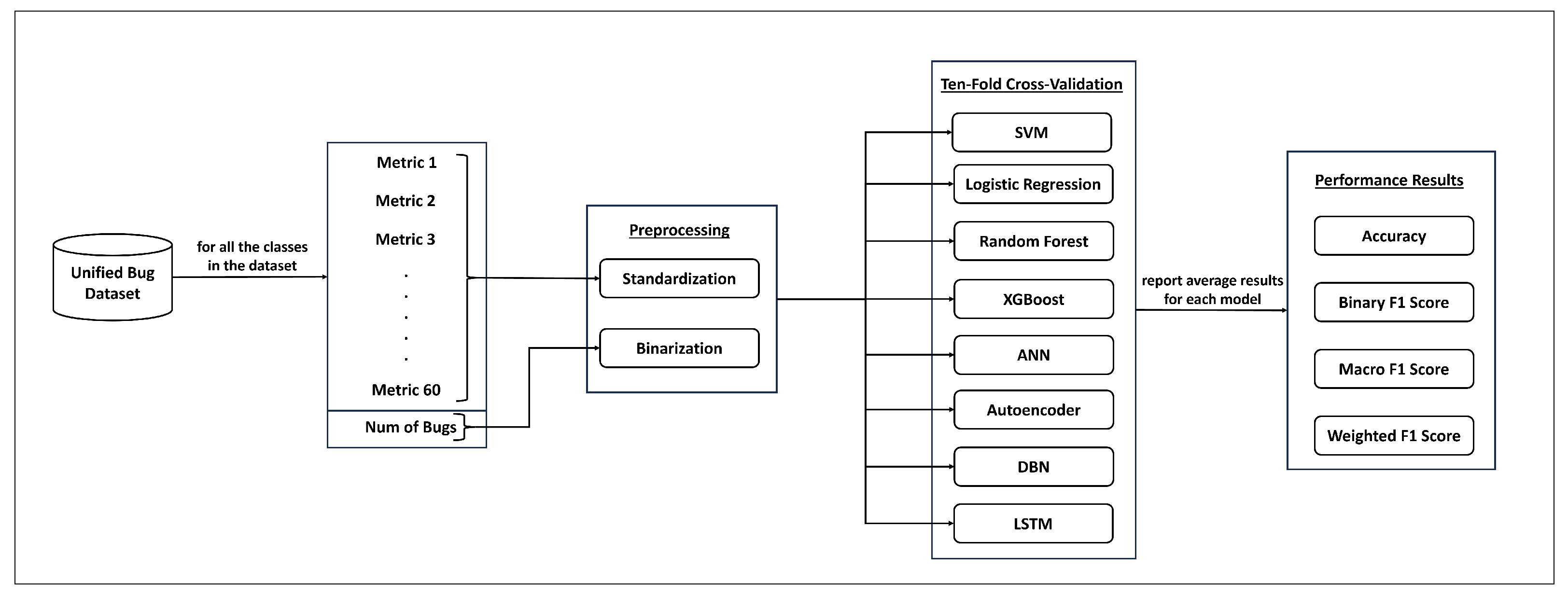
The research process used in this study is depicted in Figure 1. Initially, we preprocessed the considered dataset to improve training and the performance of bug prediction models. More details about the used dataset and preprocessing techniques are presented in Section 3.1 and Section 3.2, respectively. We used eight machine learning and deep learning approaches (see Section 3.3) to build different bug prediction models. The ten-fold cross-validation technique was used to evaluate the performance of the constructed models. According to this technique, the dataset is divided into ten subsets. Each model is trained using nine subsets, and the remaining subset is used as a validation set to evaluate the model’s performance. This procedure is repeated ten times. Each time, a different subset is selected as the validation set. Finally, the performance results obtained from each validation set are averaged to achieve a more robust evaluation of the generality of each model. The performance metrics used in our study include accuracy, binary F1 score, and weighted F1 score. The definitions of these metrics are presented in Section 3.4.
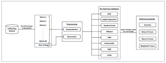
Figure 1.
The steps of our research process.
In practice, the constructed bug prediction models can be applied to real-world software systems to evaluate class quality in terms of bug-proneness. To do this, relevant features such as code metrics must be extracted from the software classes. This feature extraction process can be automated using various tools. Once the features are extracted, the bug prediction models can classify the data as either bug-prone or bug-free. This step is particularly important during the development and testing phases, especially when resources are limited, as it helps prioritize classes that require additional testing and quality improvement.
3.1. Dataset
We used the Unified Bug Dataset [30], which contains values of source-code metrics and bug information at two levels of granularity (class and file) for a broad-range set of open-source systems such as Ant, Camel, Eclipse JDP Core, and jUnit. The dataset was collected from five publicly available datasets, namely PROMISE, the Eclipse Bug Dataset, the Bug Prediction Dataset, the Bugcatchers Bug Dataset, and the GitHub Bug Dataset. The researchers [30] who collected the "Unified Bug Dataset" unified the notations and definitions of the source-code metrics reported in the original datasets, added the corresponding source code for each system in the datasets, and recalculated the values of the source-code metrics for each system using the same tool (i.e., OpenStaticAnalyzer). Finally, they created one large dataset (i.e., the Unified Bug Dataset) by combining the values of source-code metrics and bug information for 47,618 classes extracted from the systems in the original datasets. Each sample (or row) in the Unified Bug Dataset contains basic information about the class, such as the name and path of the class, values of 60 source-code metrics, and the number of bugs in the class. The source-code metrics reported in the dataset measure different aspects of internal class quality, including cohesion, coupling, complexity, documentation inheritance, and size metrics. Table 1 shows a snippet of the Unified Bug Dataset. In this study, we used these source-code metrics as features or independent variables to predict buggy and non-buggy classes (the dependent variable).

Table 1.
A snippet of the Unified Bug Dataset.
3.2. Dataset Preprocessing
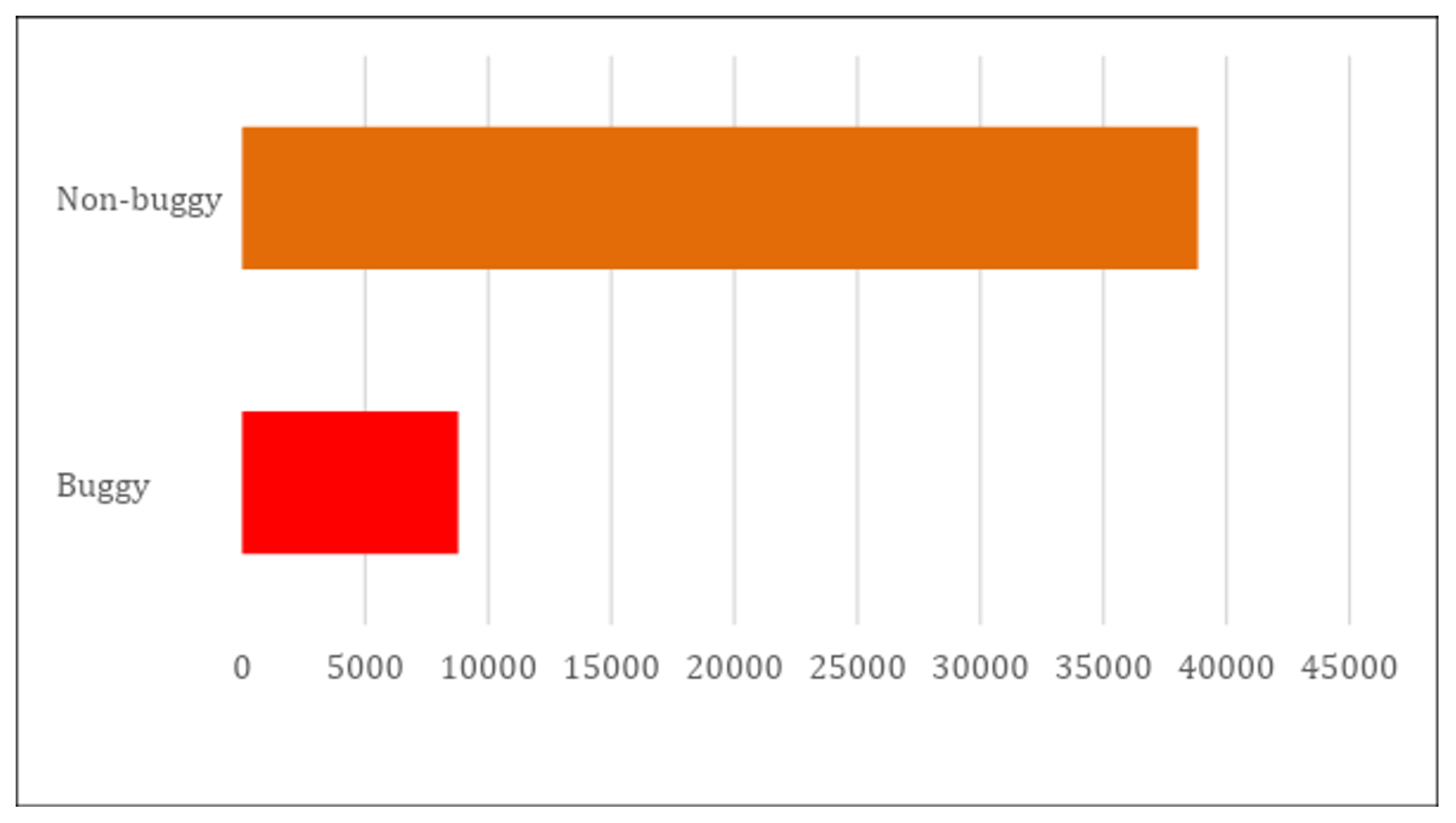
The used dataset was preprocessed using the following two techniques: binarization and standardization. We applied the binarization technique to the dependent variable corresponding to the number of bugs to convert its continuous values to binary values (0 or 1) in order to classify the data either buggy or non-buggy classes. We used this technique mainly to build prediction models for the identification of buggy and non-buggy classes. In this study, we did not aim to predict the number of bugs within a class. Data were classified as a buggy class if the number of bugs in the class was at least one or more. Otherwise, they were classified as a non-buggy class. Figure 2 shows the distribution of classes, and it can be seen that the dataset is highly imbalanced, with only 8780 buggy classes compared to 38,838 non-buggy classes.

Figure 2.
The distribution of classes in the Unified Bug Dataset.
The standardization technique was applied to the features (or the independent variables) and the sixty source-code metrics because many have different scales. It rescales the features with a mean of 0 and a variation of 1. The standardization is conducted based on the following formula:
where x is the original feature value, is the mean of the feature values, and is the standard deviation of the feature values. Standardization is an essential preprocessing step in machine learning that can improve the training and performance of models.
3.3. Machine Learning and Deep Learning Approaches
The machine and deep learning approaches used to construct bug prediction models in this research are Support Vector Machine (SVM), Logistic Regression (LR), Random Forest, Extreme Gradient Boosting (XGBoost), Artificial neural networks (ANNs), autoencoders, deep belief networks (DBNs), and long short-term memory (LSTM). A high-level description of each approach is presented as follows:
Support Vector Machine (SVM): SVM is a supervised learning approach for classification and regression tasks. It tries to find the hyperplane that optimally separates the dataset into classes, where the data points of each class reside in a different part.
Logistic Regression (LR): Logistic regression is a statistical method for predicting a binary outcome variable based on multiple predictor variables. The model is defined by the following equation:
where are the predictor variables and are the estimated regression coefficients. The magnitude of each coefficient () indicates the strength of the impact of the predictor variable () on the outcome variable. The function (q) provides the probability that the outcome variable is either 0 or 1.
Random Forest: Random forest is an ensemble learning technique that constructs multiple decision trees during training and outputs the mode of the individual trees’ classes (classification) or mean prediction (regression). It reduces overfitting by averaging multiple trees and improves accuracy and stability. Each tree is built from a random subset of the training data and features, ensuring diversity among the trees.
Extreme Gradient Boosting (XGBoost): XGBoost is an optimized implementation of the gradient-boosted trees algorithm. It builds models sequentially, with each new tree correcting the errors of the previous trees. XGBoost uses a more regularized model formalization to control overfitting and provides high performance with large datasets.
Artificial Neural Networks (ANNs): ANNs are computational models designed to mimic the structure and functioning of biological neural networks in the human brain. Typically, ANNs consist of the following three types of layers: the input layer, hidden layers, and the output layer. Each layer has a set of nodes (neurons), where each node in a given layer is connected to nodes in the next layer. ANNs learn complex patterns from data through backpropagation, a technique that adjusts the weights of connections between the nodes during training.
Autoencoders: Autoencoders are a type of ANN used as representation learning techniques. They reduce data dimensionality by encoding the input dataset as a lower-dimensional representation that captures its most essential features, then decoding it to reconstruct the original input. During training, autoencoders minimize the difference between the input and the reconstruction. They can be used in classification tasks, such as bug prediction, to remove noise and retain essential features, allowing a classifier (such as a random forest or a traditional ANN, as used in this study) to be trained on these key features.
Deep Belief Networks (DBNs): DBNs are a type of ANN used for unsupervised learning and feature extraction in deep learning. They consist of stacked layers of Restricted Boltzmann Machines (RBMs) that are initially trained separately, layer by layer, in an unsupervised manner to learn basic features of the input dataset in shallow layers and more complex features in deeper layers. DBNs can be used for classification tasks, such as bug prediction, by adding a classifier (e.g., a sigmoid classifier, as used in this study) after the final layer of the pre-trained RBMs. The entire network is then fine-tuned based on the labeled dataset.
Long Short-Term Memory (LSTM): LSTM is a type of recurrent neural network (RNN) that is better at dealing with long-term dependencies. It aims to tackle the problem of vanishing gradients in traditional RNNs by introducing memory cells that can retain information over long periods. LSTM networks are typically used in tasks where events that occur over time are essential, such as natural language processing. Additionally, they have been used in previous studies [49,50,51] in the literature to tackle different classification tasks, including maintainability prediction and bug detection.
In our experiments, we implemented all eight machine learning approaches using scikit-learn, a comprehensive library for the building of machine learning models in Python. The key hyperparameters we used in our experiments for each approach are given in Table 2.
Table 2.
Key hyperparameters for various approaches.
3.4. Evaluation
In our study, we considered four performance metrics, namely accuracy, macro F1 score, weighted F1 score, and binary F1 score, to quantitatively evaluate and compare the performance of the constructed bug prediction models. We used Accuracy because it is one of the most commonly used performance metrics in the literature on machine learning and can provide a straightforward interpretation of the performance of a model. In addition, we considered the F1 scores because our dataset is significantly imbalanced (see Figure 2). The following section provides the definitions and formulas for these metrics.
- (1)
- Accuracy: Accuracy measures the proportion of predictions that are correctly classified (i.e., true positives and true negatives) by a model, ranging from 0 to 1, where a higher value means better model performance. Accuracy is computed based on the following formula:where = true positives, = true negatives, = false positives, and = false negatives.
- (2)
- Binary F1 Score: The binary F1 score is the harmonic mean of the precision and recall metrics, emphasizing the accuracy of positive predictions. It ranges from 0 to 1, where a large value indicates better performance. The following formula is used to calculate the binary F1 score:where the formulas for precision and recall are calculated as follows:
- (3)
- Macro F1 Score: The macro F1 score is the average of the F1 scores for each class. It handles classes equally, regardless of each class’s support (i.e., the number of true instances). It is calculated using the following formula:where N is the number of classes (two classes in our case) and is the F1 score of class i.
- (4)
- Weighted F1 Score: The weighted F1 score is the weighted average of the F1 scores for each class. The average is weighted by the number of true instances in each class. The formula for the weighted F1 score is expressed as follows:where N is the number of classes, is the number of true instances for class i, and is the F1 score of class i.
4. Results and Discussions
This section presents the results of the experiments conducted following the research methodology described earlier. Eight different models were created to predict software defects. Table 3 summarizes the performance of the eight models used in the study. Accuracy, macro F1, weighted F1, and binary F1 scores were measured for each model. Next, the results of each metric are discussed across all models.
Table 3.
Performance summary.
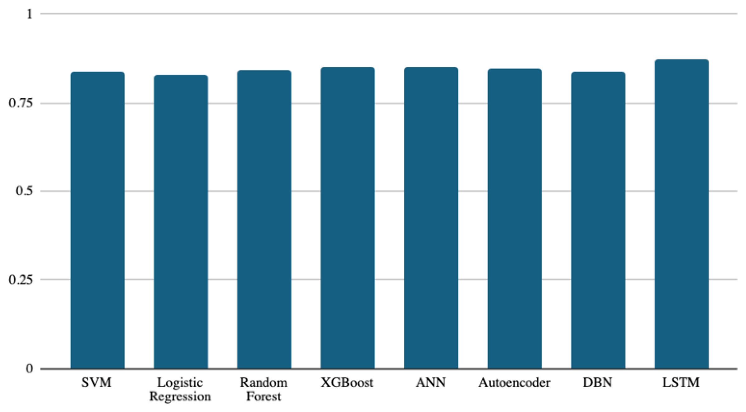
Figure 3 shows the accuracy of the models used in the study to predict buggy classes. Although the results are in a narrow range between 0.82 and 0.87, the deep learning model (LSTM) achieved the best accuracy among all models, with an accuracy score of 0.87. The ANN, XGBoost, and autoencoder models follow the LSTM model, with accuracy scores of 0.85, 0.849, and 0.846, respectively. The performance difference between these three classifiers is very slight but present. It is worth noting that even the lowest performance (logistic regression, at 0.82) is still close to that of the other models. When considering a binary classification, the performance of all classifiers is expected to be similar if the dataset is balanced. However, if the dataset has a majority class, the classifier may predict it generally. Accuracy is a simple evaluation metric for binary classification, which fits if the dataset is balanced. Therefore, we tried to use other metrics besides accuracy to compare classifiers’ performance, as presented next.

Figure 3.
Accuracy results of the eight models.
Figure 4 presents the macro F1 scores for the machine learning classifiers. The macro F1 metric is a very useful evaluation tool if the dataset is unbalanced. As discussed earlier in Figure 3, if there are slight performance differences in the accuracy of the classifiers due to imbalanced classes, the macro F1 metric is an appropriate metric that handles all dataset classes equally, regardless of balance.
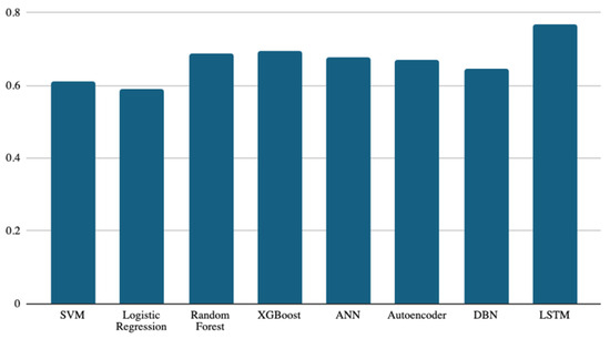
Figure 4.
Macro F1-score results of the eight models.
Again, the LSTM classifier attained the best macro F1 score of 0.76. The next best-performing classifier was XGBoost, with a macro F1 score of 0.69. The random forest, ANN, and autoencoder models were next, with scores of 0.686, 0.675, and 0.670, respectively. Again, the lowest performance was achieved by logistic regression, with a score of 0.59. The best and worst performance scores were achieved by the same classifiers for accuracy and macro F1 score. This supports the results discussed earlier in Figure 3.
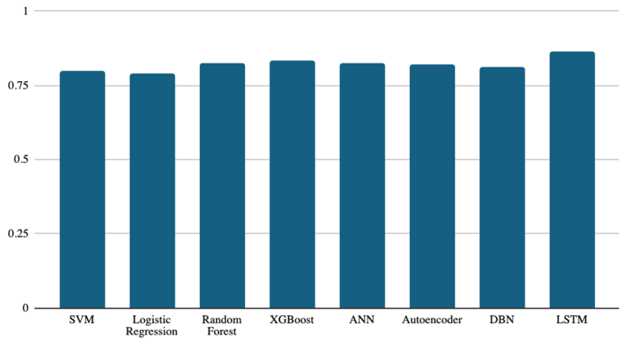
The weighted F1 scores are presented in Figure 5. This metric considers the distribution among classes in the dataset. The LSTM classifier remains the best, with a score of 0.865, followed by the XGBoost classifier, with a score of 0.831. The ANN, random forest, and autoencoder classifiers come next, with small differences between their scores of 0.826, 0.825, and 0.822, respectively. The logistic regression classifier remains at the bottom of the list, with a score of 0.787.

Figure 5.
Weighted F1-score results of the eight models.
The results of the metrics used in this study are consistent so far, with the LSTM still being the best and the logistic regression the worst-performing model among all classifiers compared in this study.
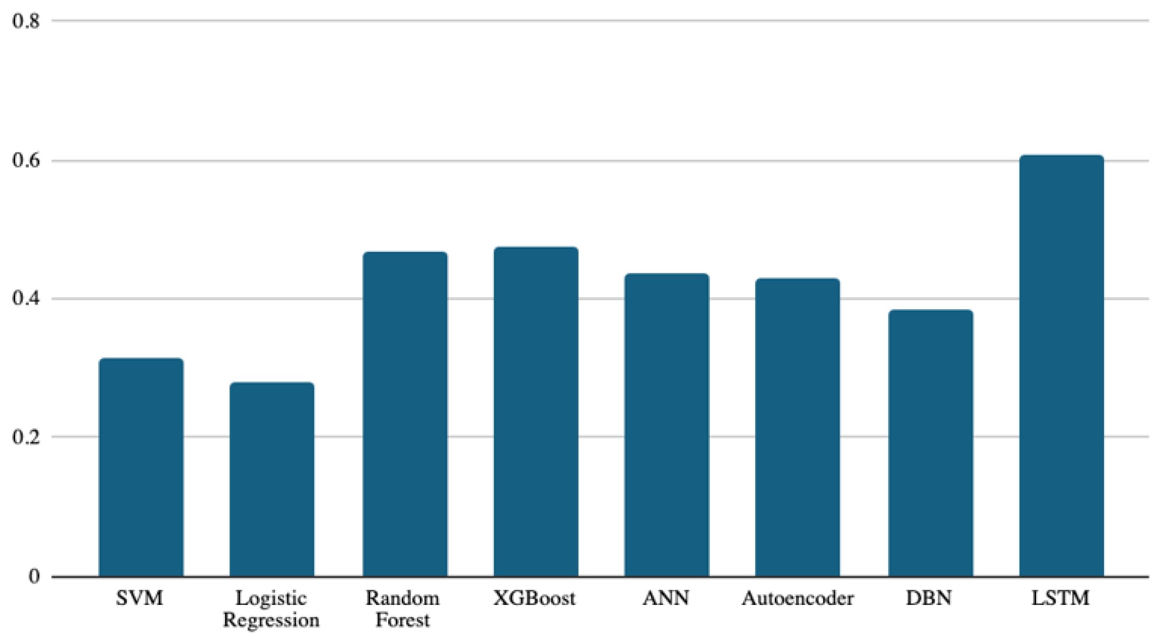
The binary F1, as shown in Figure 6, is the last metric used for classifier performance evaluation. It is worth noting that the LSTM is still the best classifier, with a score of 0.608, and logistic regression remains at the bottom among all classifiers, with a score of 0.279. The rest of the classifiers were in the middle, with score ranges between 0.474 and 0.314.

Figure 6.
Binary F1-score results of the eight models.
The binary F1 score combines the precision and recall metrics. While the accuracy metric might be affected by unbalanced data, the F1 score can control this effect by combining the precision and recall metrics. Despite the current study using four different evaluation metrics (accuracy and macro, micro, and binary F1 scores), the results are consistent, and the LSTM classifier achieved the best performance using these four metrics.
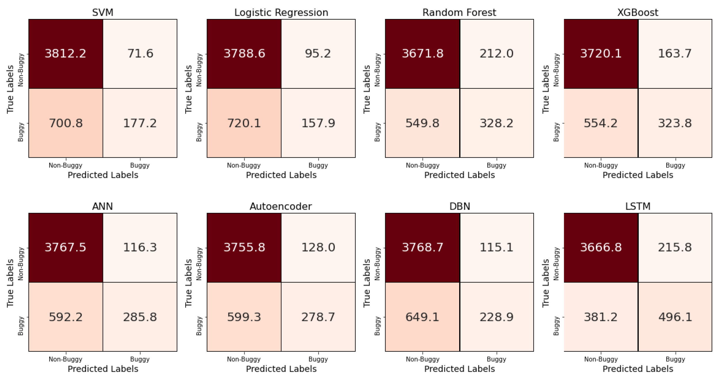
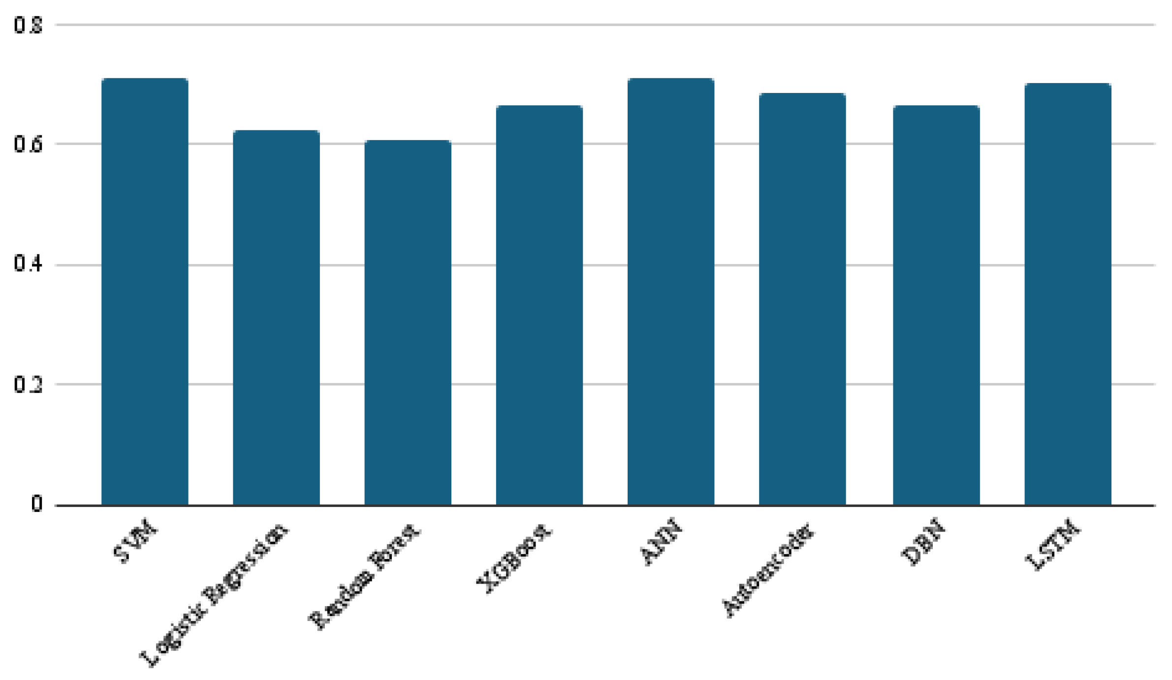
In addition to the results of the main four performance metrics discussed above, the average confusion matrix, precision, and recall obtained from the ten-fold cross-validation for each of the eight models are presented in Figure 7, Figure 8 and Figure 9, respectively. The confusion matrices offer valuable insight into the distribution of true positives and false negatives, revealing that the LSTM model consistently minimized misclassifications of bug-prone classes compared to other models. SVM and ANN achieved the best precision results, with a score of 0.71, while LSTM followed closely, at 0.70. For recall, LSTM significantly outperformed all other classifiers, with a score of 0.55, which is 18 points ahead of the next-best models, namely random forest and XGBoost. These findings demonstrate LSTM’s superior ability to capture bug-prone classes compared to the considered models, particularly in terms of recall, which emphasizes its strength in identifying bug-prone instances, even in imbalanced datasets.
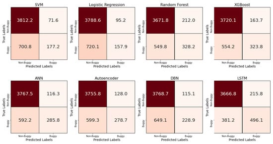
Figure 7.
Average confusion matrix for each the eight models obtained with a ten-fold cross-validation.

Figure 8.
Precision results of the eight models.
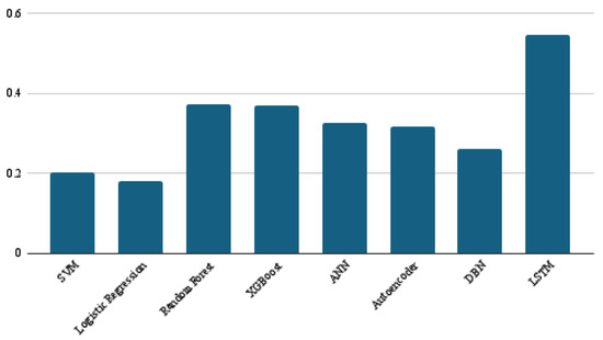
Figure 9.
Recall results of the eight models.
5. Conclusions and Future Work
In conclusion, early bug prediction is pivotal to increasing software reliability and reducing maintenance costs. This study employed eight machine learning and deep learning techniques to construct bug prediction models using the Unified Bug dataset, which contains bug information and 60 software metrics for 47,618 classes extracted from a wide range of open-source systems. We preprocessed the dataset by applying standardization and converting the bug information into a binary class. The performance of the prediction models was evaluated using accuracy, macro F1 score, weighted F1 score, and binary F1 score. Our empirical results show that the LSTM deep learning technique outperformed the other considered techniques, indicating its potential usefulness in the context of software bug prediction. This is an important finding because most studies in the literature have used traditional and ensemble machine learning techniques for bug prediction. Therefore, we recommend further investigations into the use of deep learning techniques such as LSTM to predict the occurrence of software bugs.
In future work, several directions can be considered to extend this study. An empirical investigation could explore the impact of applying feature selection techniques on the performance of the machine learning and deep learning methods used in this study with the Unified Bug Dataset. Additionally, further investigations and experiments could be conducted to fine tune the hyperparameters of such techniques to identify the configurations that achieve the best performance for each method in bug prediction. Finally, many hybrid classification models that combine different machine learning and deep learning techniques could be developed and empirically evaluated to improve the accuracy of bug prediction.
Author Contributions
Conceptualization, W.A. and M.A.; methodology, M.A.; software, M.A.; validation, W.A. and M.A.; formal analysis, W.A.; investigation, W.A. and M.A; resources, W.A. and M.A.; data curation, M.A.; writing—original draft preparation, W.A.; writing—review and editing, W.A. and M.A.; visualization, M.A.; supervision, W.A.; project administration, W.A. All authors have read and agreed to the published version of the manuscript.
Funding
This research received no external funding.
Institutional Review Board Statement
Not applicable.
Informed Consent Statement
Not applicable.
Data Availability Statement
Dataset available on request from the authors.
Acknowledgments
The Researchers would like to thank the Deanship of Graduate Studies and Scientific Research at Qassim University for financial support (QU-APC-2024-9/1).
Conflicts of Interest
The authors declare no conflicts of interest.
References
- Malhotra, R.; Chug, A. Software maintainability: Systematic literature review and current trends. Int. J. Softw. Eng. Knowl. Eng. 2016, 26, 1221–1253. [Google Scholar] [CrossRef]
- Huang, Q.; Shihab, E.; Xia, X.; Lo, D.; Li, S. Identifying self-admitted technical debt in open source projects using text mining. Empir. Softw. Eng. 2018, 23, 418–451. [Google Scholar] [CrossRef]
- Guo, J.; Yang, D.; Siegmund, N.; Apel, S.; Sarkar, A.; Valov, P.; Czarnecki, K.; Wasowski, A.; Yu, H. Data-efficient performance learning for configurable systems. Empir. Softw. Eng. 2018, 23, 1826–1867. [Google Scholar] [CrossRef]
- Boussaïd, I.; Siarry, P.; Ahmed-Nacer, M. A survey on search-based model-driven engineering. Autom. Softw. Eng. 2017, 24, 233–294. [Google Scholar] [CrossRef]
- Gondra, I. Applying machine learning to software fault-proneness prediction. J. Syst. Softw. 2008, 81, 186–195. [Google Scholar] [CrossRef]
- Iyer, S.; Konstas, I.; Cheung, A.; Zettlemoyer, L. Summarizing source code using a neural attention model. In Proceedings of the 54th Annual Meeting of the Association for Computational Linguistics 2016, Berlin, Germany, 7–12 August 2016; Association for Computational Linguistics: Kerrville, TX, USA, 2016; pp. 2073–2083. [Google Scholar]
- Mishra, S.; Sharma, A. Maintainability prediction of object oriented software by using adaptive network based fuzzy system technique. Int. J. Comput. Appl. 2015, 119, 24–27. [Google Scholar] [CrossRef]
- Ahmed, M.A.; Al-Jamimi, H.A. Machine learning approaches for predicting software maintainability: A fuzzy-based transparent model. IET Softw. 2013, 7, 317–326. [Google Scholar] [CrossRef]
- Mohd Adnan, M.; Sarkheyli, A.; Mohd Zain, A.; Haron, H. Fuzzy logic for modeling machining process: A review. Artif. Intell. Rev. 2015, 43, 345–379. [Google Scholar] [CrossRef]
- Chhabra, J.K. Improving package structure of object-oriented software using multi-objective optimization and weighted class connections. J. King Saud-Univ.-Comput. Inf. Sci. 2017, 29, 349–364. [Google Scholar]
- Elish, M.O.; Aljamaan, H.; Ahmad, I. Three empirical studies on predicting software maintainability using ensemble methods. Soft Comput. 2015, 19, 2511–2524. [Google Scholar] [CrossRef]
- Finlay, J.; Pears, R.; Connor, A.M. Data stream mining for predicting software build outcomes using source-code metrics. Inf. Softw. Technol. 2014, 56, 183–198. [Google Scholar] [CrossRef]
- Francese, R.; Risi, M.; Scanniello, G.; Tortora, G. Proposing and assessing a software visualization approach based on polymetric views. J. Vis. Lang. Comput. 2016, 34, 11–24. [Google Scholar] [CrossRef]
- Huo, X.; Li, M.; Zhou, Z.H. Learning unified features from natural and programming languages for locating buggy source code. In Proceedings of the IJCAI, New York, NY, USA, 9–15 July 2016; Volume 16, pp. 1606–1612. [Google Scholar]
- Haije, T.; Intelligentie, B.O.K.; Gavves, E.; Heuer, H. Automatic comment generation using a neural translation model. Inf. Softw. Technol. 2016, 55, 258–268. [Google Scholar]
- Ionescu, V.S.; Demian, H.; Czibula, I.G. Natural language processing and machine learning methods for software development effort estimation. Stud. Inform. Control 2017, 26, 219–228. [Google Scholar] [CrossRef]
- Jamshidi, P.; Siegmund, N.; Velez, M.; Kästner, C.; Patel, A.; Agarwal, Y. Transfer learning for performance modeling of configurable systems: An exploratory analysis. In Proceedings of the 2017 32nd IEEE/ACM International Conference on Automated Software Engineering (ASE), Urbana, IL, USA, 30 October–3 November 2017; pp. 497–508. [Google Scholar]
- Kaur, A.; Kaur, K. Statistical comparison of modelling methods for software maintainability prediction. Int. J. Softw. Eng. Knowl. Eng. 2013, 23, 743–774. [Google Scholar] [CrossRef]
- Li, L.; Feng, H.; Zhuang, W.; Meng, N.; Ryder, B. Cclearner: A deep learning-based clone detection approach. In Proceedings of the 2017 IEEE international conference on software maintenance and evolution (ICSME), Shanghai, China, 17–22 September 2017; pp. 249–260. [Google Scholar]
- Laradji, I.H.; Alshayeb, M.; Ghouti, L. Software defect prediction using ensemble learning on selected features. Inf. Softw. Technol. 2015, 58, 388–402. [Google Scholar] [CrossRef]
- Lin, M.J.; Yang, C.Z.; Lee, C.Y.; Chen, C.C. Enhancements for duplication detection in bug reports with manifold correlation features. J. Syst. Softw. 2016, 121, 223–233. [Google Scholar] [CrossRef]
- Luo, Q.; Nair, A.; Grechanik, M.; Poshyvanyk, D. Forepost: Finding performance problems automatically with feedback-directed learning software testing. Empir. Softw. Eng. 2017, 22, 6–56. [Google Scholar] [CrossRef]
- Menzies, T.; Greenwald, J.; Frank, A. Data mining static code attributes to learn defect predictors. IEEE Trans. Softw. Eng. 2006, 33, 2–13. [Google Scholar] [CrossRef]
- Malhotra, R.; Khanna, M. An exploratory study for software change prediction in object-oriented systems using hybridized techniques. Autom. Softw. Eng. 2017, 24, 673–717. [Google Scholar] [CrossRef]
- Malhotra, R. A systematic review of machine learning techniques for software fault prediction. Appl. Soft Comput. 2015, 27, 504–518. [Google Scholar] [CrossRef]
- Radjenović, D.; Heričko, M.; Torkar, R.; Živkovič, A. Software fault prediction metrics: A systematic literature review. Inf. Softw. Technol. 2013, 55, 1397–1418. [Google Scholar] [CrossRef]
- Rahimi, S.; Zargham, M. Vulnerability scrying method for software vulnerability discovery prediction without a vulnerability database. IEEE Trans. Reliab. 2013, 62, 395–407. [Google Scholar] [CrossRef]
- Tavakoli, H.R.; Borji, A.; Laaksonen, J.; Rahtu, E. Exploiting inter-image similarity and ensemble of extreme learners for fixation prediction using deep features. Neurocomputing 2017, 244, 10–18. [Google Scholar] [CrossRef]
- Yang, X.; Lo, D.; Xia, X.; Sun, J. TLEL: A two-layer ensemble learning approach for just-in-time defect prediction. Inf. Softw. Technol. 2017, 87, 206–220. [Google Scholar] [CrossRef]
- Ferenc, R.; Tóth, Z.; Ladányi, G.; Siket, I.; Gyimóthy, T. A public unified bug dataset for java and its assessment regarding metrics and bug prediction. Softw. Qual. J. 2020, 28, 1447–1506. [Google Scholar] [CrossRef]
- Jureczko, M.; Madeyski, L. Towards identifying software project clusters with regard to defect prediction. In Proceedings of the 6th International Conference on Predictive Models in Software Engineering, Timisoara, Romania, 12–13 September 2010; pp. 1–10. [Google Scholar]
- Zimmermann, T.; Premraj, R.; Zeller, A. Predicting defects for eclipse. In Proceedings of the Third International Workshop on Predictor Models in Software Engineering (PROMISE’07: ICSE Workshops 2007), Minneapolis, MN, USA, 20–26 May 2007; p. 9. [Google Scholar]
- D’Ambros, M.; Lanza, M.; Robbes, R. An extensive comparison of bug prediction approaches. In Proceedings of the 2010 7th IEEE Working Conference on Mining Software Repositories (MSR 2010), Cape Town, South Africa, 2–3 May 2010; pp. 31–41. [Google Scholar]
- Hall, T.; Zhang, M.; Bowes, D.; Sun, Y. Some code smells have a significant but small effect on faults. ACM Trans. Softw. Eng. Methodol. (TOSEM) 2014, 23, 1–39. [Google Scholar] [CrossRef]
- Tóth, Z.; Gyimesi, P.; Ferenc, R. A public bug database of github projects and its application in bug prediction. In Proceedings of the Computational Science and Its Applications—ICCSA 2016: 16th International Conference, Beijing, China, 4–7 July 2016; Proceedings, Part IV 16. Springer: Berlin, Heidelberg, Germany, 2016; pp. 625–638. [Google Scholar]
- Dong, X.; Liang, Y.; Miyamoto, S.; Yamaguchi, S. Ensemble learning based software defect prediction. J. Eng. Res. 2023, 11, 377–391. [Google Scholar] [CrossRef]
- Khleel, N.A.A.; Nehéz, K. Comprehensive study on machine learning techniques for software bug prediction. Int. J. Adv. Comput. Sci. Appl. 2021, 12, 8. [Google Scholar] [CrossRef]
- Ibrahim, A.M.; Abdelsalam, H.; Taj-Eddin, I.A. Software Defects Prediction At Method Level Using Ensemble Learning Techniques. Int. J. Intell. Comput. Inf. Sci. 2023, 23, 28–49. [Google Scholar] [CrossRef]
- Hammouri, A.; Hammad, M.; Alnabhan, M.; Alsarayrah, F. Software bug prediction using machine learning approach. Int. J. Adv. Comput. Sci. Appl. 2018, 9, 2. [Google Scholar] [CrossRef]
- Subbiah, U.; Ramachandran, M.; Mahmood, Z. Software engineering approach to bug prediction models using machine learning as a service (MLaaS). In Proceedings of the Icsoft 2018—Proceedings of the 13th International Conference on Software Technologies, Porto, Portugal, 26–28 July 2018; pp. 879–887. [Google Scholar]
- Khalid, A.; Badshah, G.; Ayub, N.; Shiraz, M.; Ghouse, M. Software defect prediction analysis using machine learning techniques. Sustainability 2023, 15, 5517. [Google Scholar] [CrossRef]
- Alzahrani, M. Using Machine Learning Techniques to Predict Bugs in Classes: An Empirical Study. Int. J. Adv. Comput. Sci. Appl. 2022, 13. [Google Scholar] [CrossRef]
- Marçal, I.; Garcia, R.E. Bug Prediction Models: Seeking the most efficient. 2024. preprint. Available online: https://www.researchsquare.com/article/rs-3900175/v1 (accessed on 20 September 2024).
- Jha, S.; Kumar, R.; Abdel-Basset, M.; Priyadarshini, I.; Sharma, R.; Long, H.V. Deep learning approach for software maintainability metrics prediction. IEEE Access 2019, 7, 61840–61855. [Google Scholar] [CrossRef]
- Yu, T.Y.; Huang, C.Y.; Fang, N.C. Use of deep learning model with attention mechanism for software fault prediction. In Proceedings of the 2021 8th International Conference on Dependable Systems and Their Applications (DSA), Yinchuan, China, 11–12 September 2021; pp. 161–171. [Google Scholar]
- Qiao, L.; Li, X.; Umer, Q.; Guo, P. Deep learning based software defect prediction. Neurocomputing 2020, 385, 100–110. [Google Scholar] [CrossRef]
- Alghanim, F.; Azzeh, M.; El-Hassan, A.; Qattous, H. Software defect density prediction using deep learning. IEEE Access 2022, 10, 114629–114641. [Google Scholar] [CrossRef]
- Al Qasem, O.; Akour, M.; Alenezi, M. The influence of deep learning algorithms factors in software fault prediction. IEEE Access 2020, 8, 63945–63960. [Google Scholar] [CrossRef]
- Tatsunami, Y.; Taki, M. Sequencer: Deep lstm for image classification. Adv. Neural Inf. Process. Syst. 2022, 35, 38204–38217. [Google Scholar]
- Liu, Q.; Zhou, F.; Hang, R.; Yuan, X. Bidirectional-convolutional LSTM based spectral-spatial feature learning for hyperspectral image classification. Remote Sens. 2017, 9, 1330. [Google Scholar] [CrossRef]
- Teshima, Y.; Watanobe, Y. Bug detection based on lstm networks and solution codes. In Proceedings of the 2018 IEEE International Conference on Systems, Man, and Cybernetics (SMC), Miyazaki, Japan, 7–10 October 2018; pp. 3541–3546. [Google Scholar]


Disclaimer/Publisher’s Note: The statements, opinions and data contained in all publications are solely those of the individual author(s) and contributor(s) and not of MDPI and/or the editor(s). MDPI and/or the editor(s) disclaim responsibility for any injury to people or property resulting from any ideas, methods, instructions or products referred to in the content. |
© 2024 by the authors. Licensee MDPI, Basel, Switzerland. This article is an open access article distributed under the terms and conditions of the Creative Commons Attribution (CC BY) license (https://creativecommons.org/licenses/by/4.0/).