
A Simplified One-Parallel-Element Automatic Impedance-Matching Network Applied to Electromagnetic Acoustic Transducers Driving †

Abstract
:1. Introduction
Contribution
2. Backgound Theory
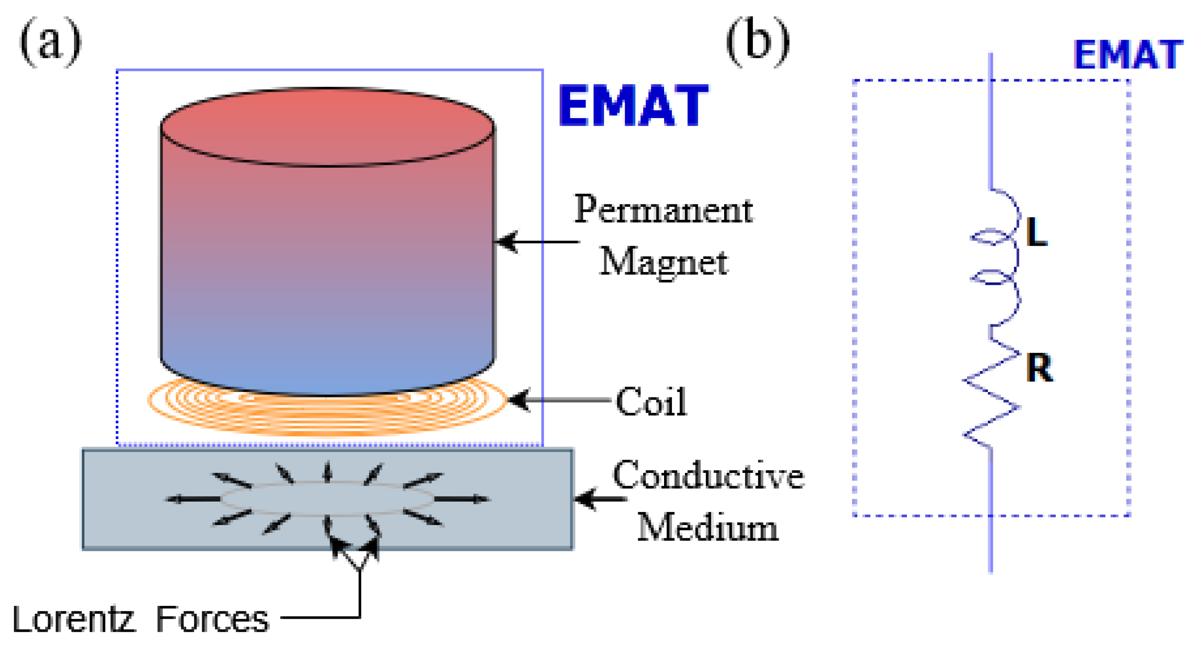
2.1. Ultrasonic Waves and Electromagnetic Acoustic Transducer
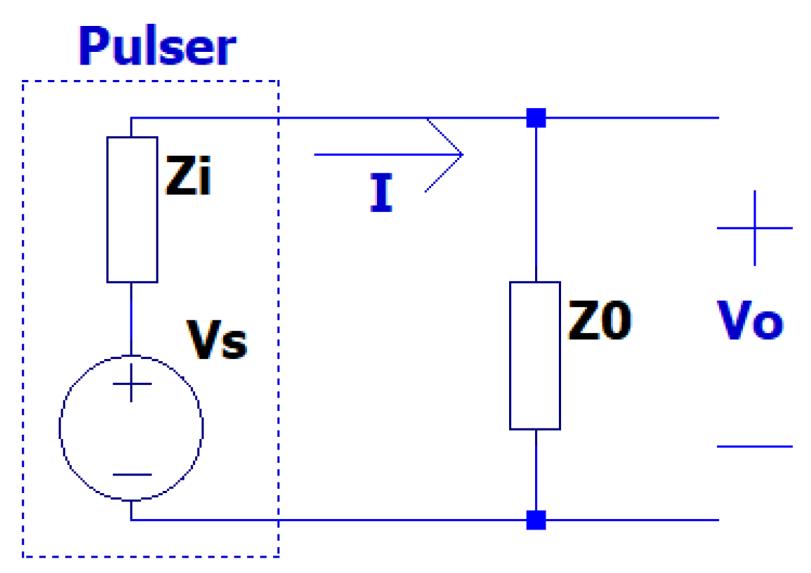
2.2. Maximum Power Transfer Theorem
3. Impedance-Matching Networks
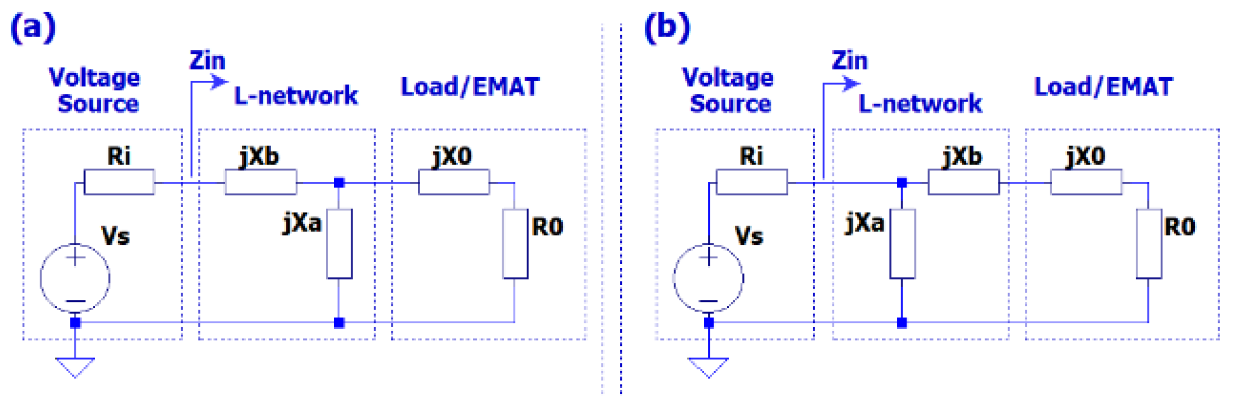
3.1. L-Networks
3.2. Simplified One-Parallel-Element ()
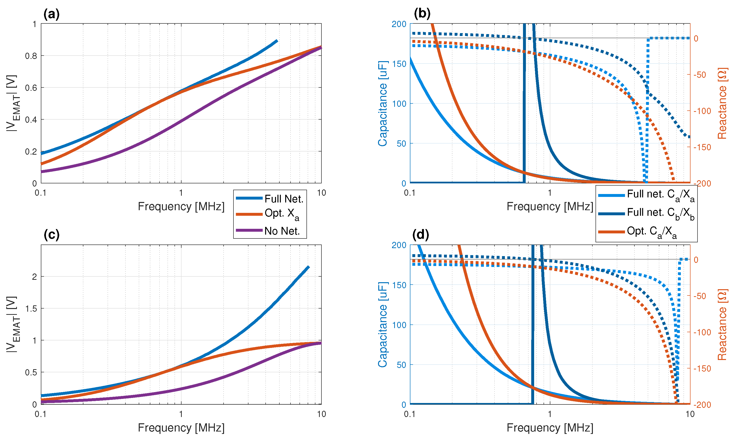
4. EMAT Impedance-Matching Theoretical Assessment
5. Experimental Validation
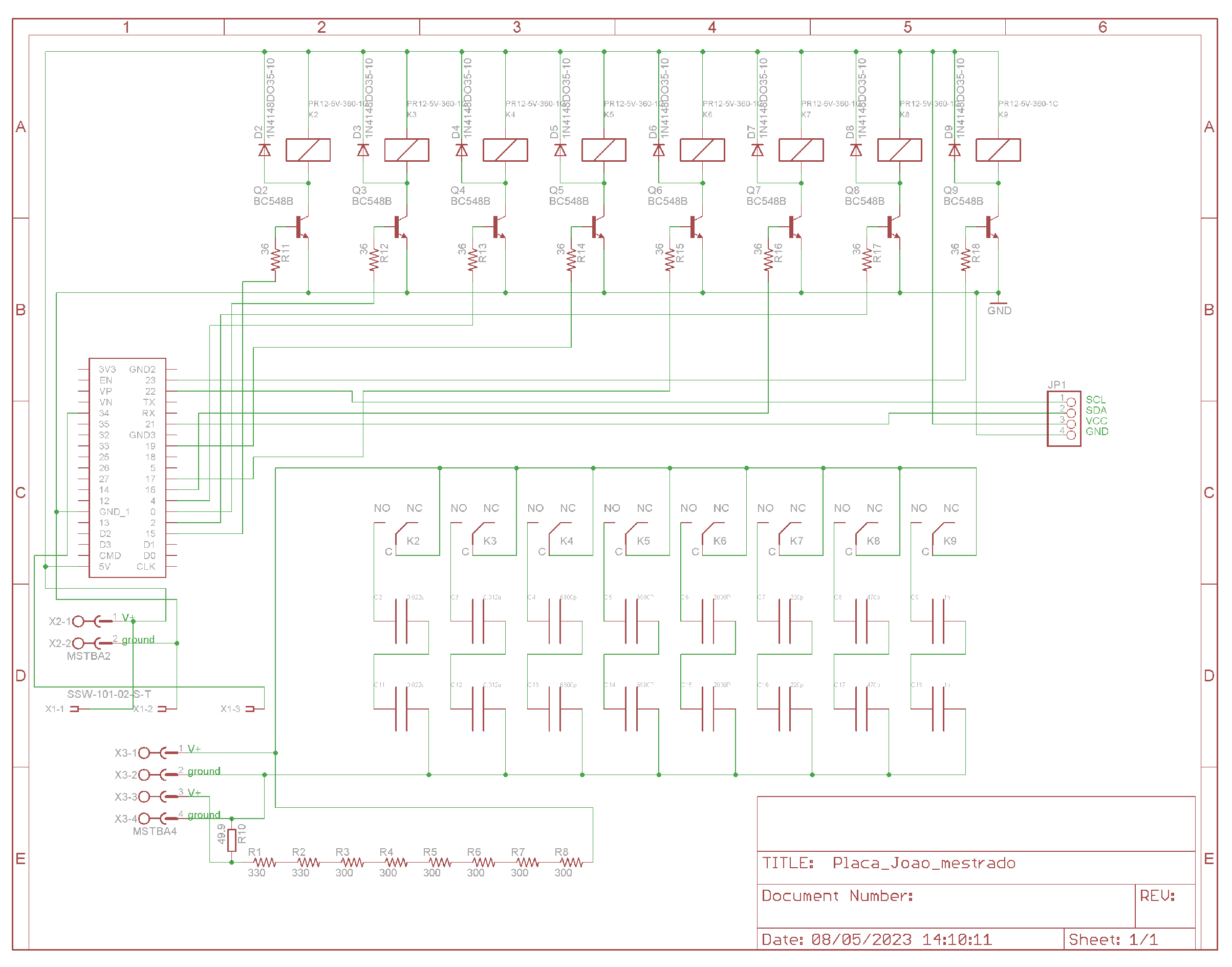
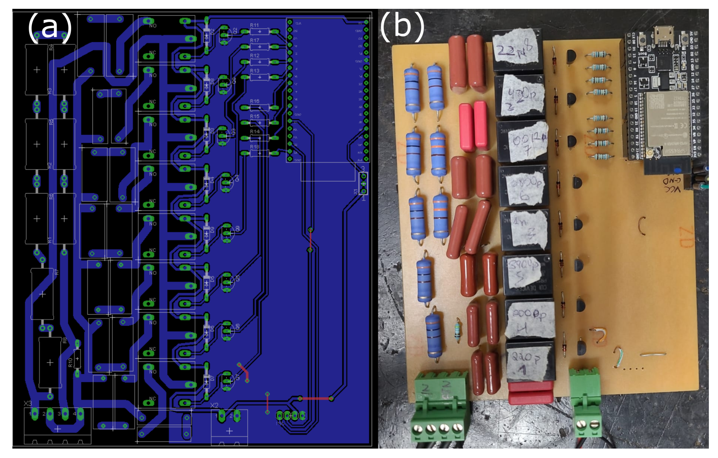
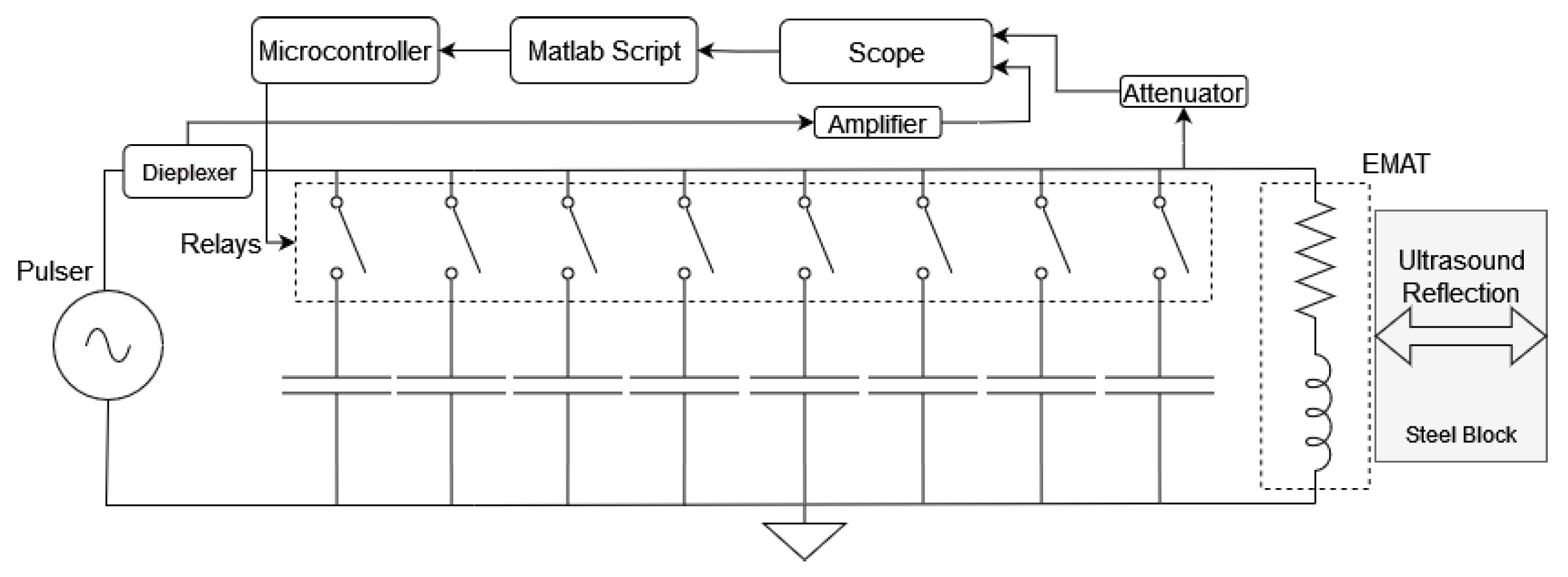
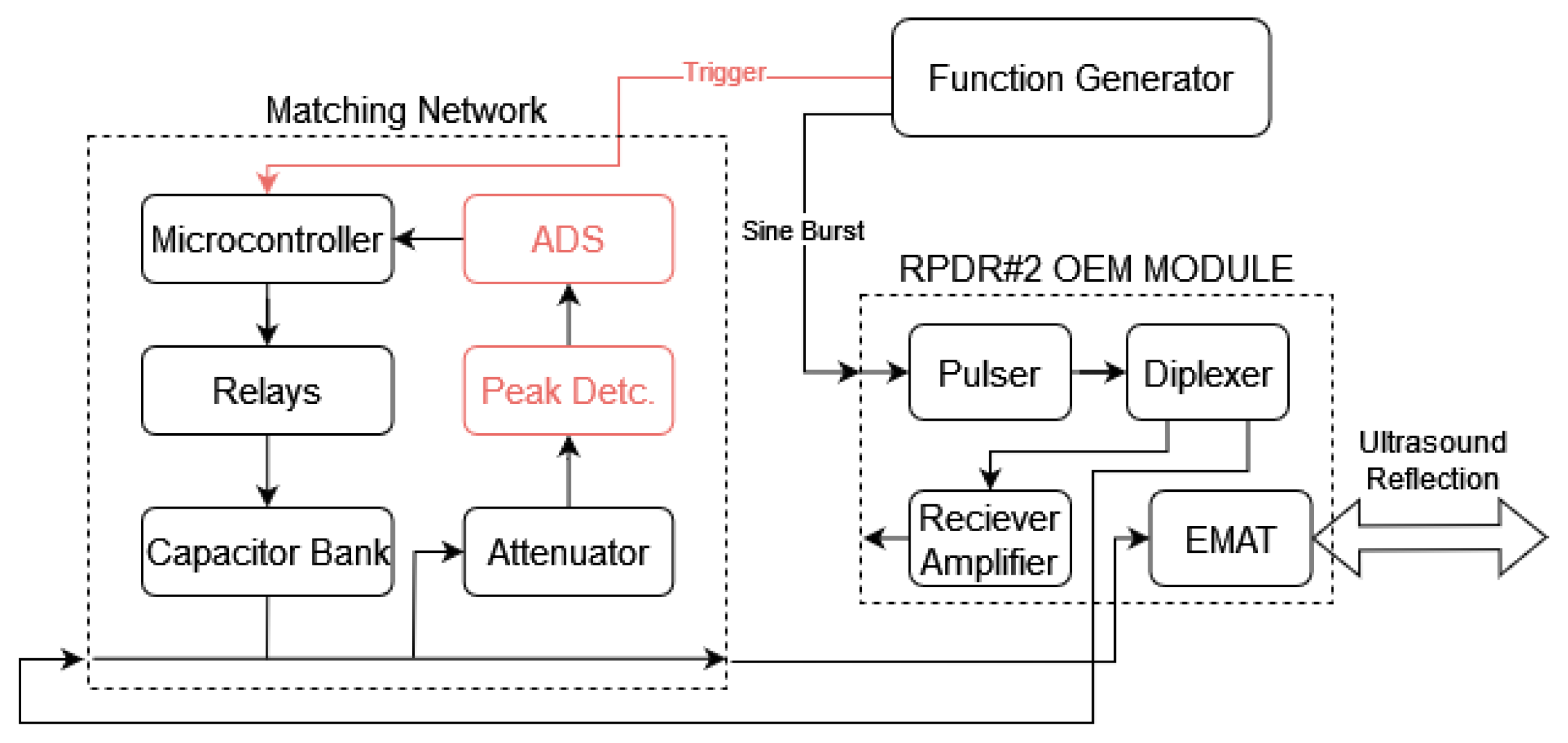
5.1. Experimental Setup
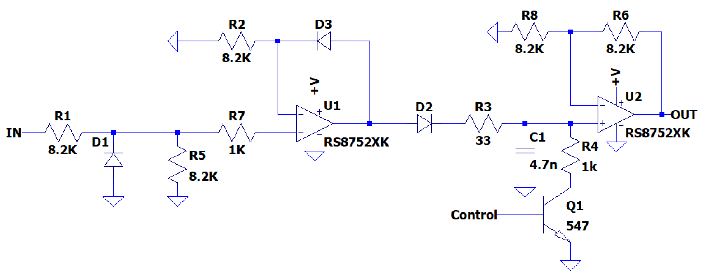
Hardware Peak Detector
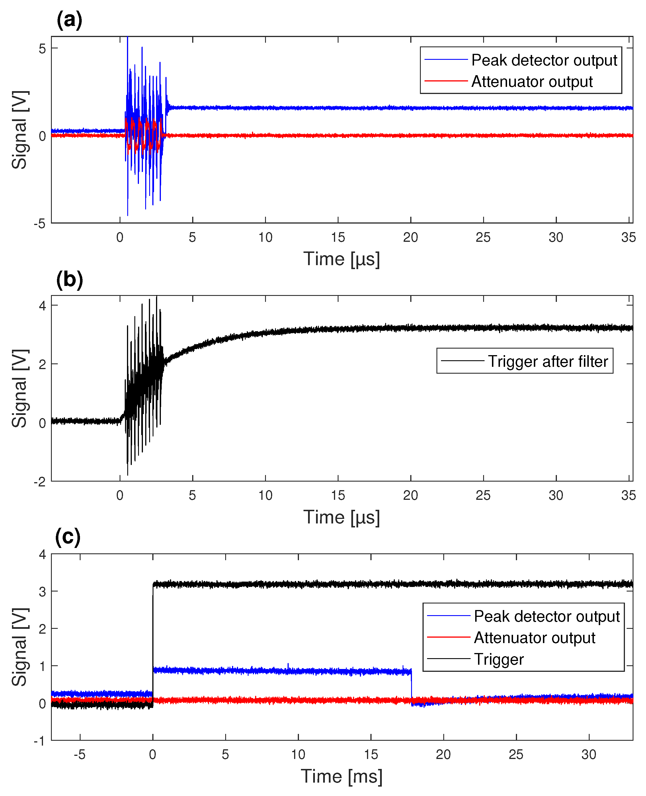
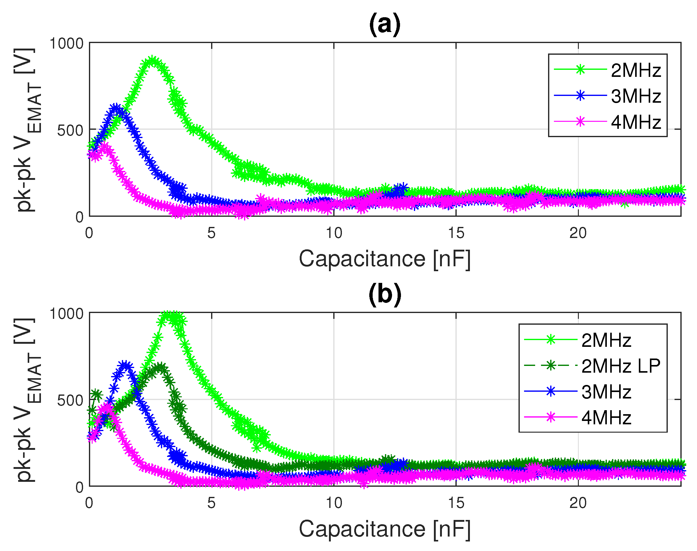
5.2. Experimental Results
Hardware Peak Detector
6. Conclusions
Author Contributions
Funding
Institutional Review Board Statement
Data Availability Statement
Acknowledgments
Conflicts of Interest
References
- Schmerr, L.W. Fundamentals of Ultrasonic Nondestructive Evaluation: A Modeling Approach; Springer: Berlin/Heidelberg, Germany, 2016. [Google Scholar]
- Kubrusly, A.C.; Dixon, S. Application of the reciprocity principle to evaluation of mode-converted scattered shear horizontal (SH) wavefields in tapered thinning plates. Ultrasonics 2021, 117, 106544. [Google Scholar] [CrossRef] [PubMed]
- Hirao, M.; Ogi, H. EMATs for Science and Industry: Noncontacting Ultrasonic Measurements; Springer: Berlin/Heidelberg, Germany, 2017. [Google Scholar]
- Rose, J.L. Ultrasonic Guided Waves in Solid Media; Cambridge University Press: Cambridge, UK, 2014. [Google Scholar]
- Cheeke, J.N.D. Fundamentals and Applications of Ultrasonic Waves, 2nd ed.; CRC Press: Boca Raton, FL, USA, 2017. [Google Scholar]
- Miao, H.; Li, F. Shear horizontal wave transducers for structural health monitoring and nondestructive testing: A review. Ultrasonics 2021, 114, 106355. [Google Scholar] [CrossRef] [PubMed]
- Rose, J.L.; Jiao, D.; Spanner, J. Ultrasonics Guided Waves for Piping Inspection. In Review of Progress in Quantitative Nondestructive Evaluation; Thompson, D.O., Chimenti, D.E., Eds.; Springer: Boston, MA, USA, 1997; Volume 16A, pp. 1285–1290. [Google Scholar]
- Maxfield, Z.W.B. Electromagnetic Acoustic Transducers for Nondestructive Evaluation. In ASM Handbook, Volume 17: Nondestructive Evaluation of Materials; Ahmad, A., Bond, L.J., Eds.; ASM International: Novelty, OH, USA, 2018. [Google Scholar]
- Wu, Y.; Wu, Y. The Effect of Magnet-to-Coil Distance on the Performance Characteristics of EMATs. Sensors 2020, 20, 5096. [Google Scholar] [CrossRef] [PubMed]
- Ding, X.; Hong, B.; Wu, X.; He, L. Lift-off Performance of Receiving EMAT Transducer Enhanced by Voltage Resonance. In Proceedings of the 18th World Conference on Nondestructive Testing, Durban, South Africa, 16–20 April 2012. [Google Scholar]
- Wenze, S.; Chen, W.; Lu, C.; Zhang, J.; Chen, Y.; Xu, W. Optimal Design of Spiral Coil EMATs for Improving Their Pulse Compression Effect. J. Nondestruct. Eval. 2021, 40, 38. [Google Scholar]
- Zao, Y.; Ouyang, Q.; Zhang, X.; Hou, S.; Fang, M. The dynamic impedance matching method for high temperature electromagnetic acoustic transducer. In Proceedings of the 2017 29th Chinese Control and Decision Conference (CCDC), Chongqing, China, 28–30 May 2017; pp. 1923–1927. [Google Scholar]
- Kong, C. A general maximum power transfer theorem. IEEE Trans. Educ. 1995, 38, 296–298. [Google Scholar] [CrossRef]
- Kuang, Y.; Jin, Y.; Cochran, S.; Huang, Z. Resonance tracking and vibration stablilization for high power ultrasonic transducers. Ultrasonics 2014, 54, 187–194. [Google Scholar] [CrossRef] [PubMed]
- Wang, J.; Wu, X.; Song, Y.; Sun, L. Study of the Influence of the Backplate Position on EMAT Thickness-Measurement Signals. Sensors 2022, 12, 8741. [Google Scholar] [CrossRef] [PubMed]
- Pozar, D.M. Microwave Engineering, 4th ed.; University of Massashussets at Amhert: Amherst, MA, USA, 2012; Chapters 2.6 and 5.1. [Google Scholar]
- Jian, X.; Dixon, S.; Edwards, R.; Morrison, J. Coupling mechanism of an EMAT. Ultrasonics 2006, 44, e653–e656. [Google Scholar] [CrossRef] [PubMed]
- Chuck, H. Handbook of Nondestructive Evaluation, 2nd ed.; McGraw Hill Professional: New York, NY, USA, 2012. [Google Scholar]
- Sekhar, P.; Uwizeye, V. 2—Review of sensor and actuator mechanisms for bioMEMS. In MEMS for Biomedical Applications; Bhansali, S., Vasudev, A., Eds.; Woodhead Publishing: Sawston, UK, 2012; pp. 46–77. [Google Scholar]
- Kuperman, W.A. Underwater Acoustics. In Encyclopedia of Physical Science and Technology, 3rd ed.; Meyers, R.A., Ed.; Academic Press: Cambridge, MA, USA, 2003; pp. 317–338. [Google Scholar]
- Ribichini, R. Modelling of Electromagnetic Acoustic Transducers. Ph.D. Thesis, Imperial College London, London, UK, 2011. [Google Scholar]
- Allam, A.; Bhardwaj, A.; Sabra, K.; Erturk, A. Piezoelectric transducer design and impedance tuning for concurrent ultrasonic power and data transfer. In Active and Passive Smart Structures and Integrated Systems XVI; Han, J.H., Shahab, S., Yang, J., Eds.; Society of Photo-Optical Instrumentation Engineers (SPIE) Conference Series; SPIE: Long Beach, CA, USA, 2022. [Google Scholar]
- Agarwal, A.; Lang, J.H. Foundations of Analog and Digital Electronic Circuits; Morgan Kaufmann Publishers: San Francisco, CA, USA, 2005. [Google Scholar]
- Torres de Sousa Andrade, J.P.; Suzano Medeiros, V.; Kubrusly, A.C. A simplified automatic impedance matching network for electromagnetic acoustic transducers. In Proceedings of the 2023 7th International Symposium on Instrumentation Systems, Circuits and Transducers (INSCIT), Rio de Janeiro, Brazil, 28 August–1 September 2023; pp. 1–6. [Google Scholar] [CrossRef]
- Metallized Polypropylene Film Capacitors ECWH(A) Series. Available online: https://industrial.panasonic.com/cdbs/www-data/pdf/RDI0000/ABD0000C187.pdf (accessed on 12 July 2023).
- Metaltex Miniature Relay. Available online: https://www.metaltex.com.br/assets/produtos/pdf/ax.pdf (accessed on 2 May 2023).
- ESP32-WROVER-I and ESP32-WROVER-IE Datasheet. Available online: https://www.espressif.com/sites/default/files/documentation/esp32-wrover-e_esp32-wrover-ie_datasheet_en.pdf (accessed on 25 January 2023).
- Ultra-Small, Low-Power, 12-Bit Analog-to-Digital Converter with Internal Reference. Available online: https://cdn-shop.adafruit.com/datasheets/ads1015.pdf (accessed on 30 April 2023).
- Kelley, H.; Alonso, G. LTC6244 High Speed Peak Detector. Available online: https://www.analog.com/en/technical-articles/ltc6244-high-speed-peak-detector.html (accessed on 2 May 2023).
- Irazabal, J.; Blozis, S. Application Note AN10216-01 I2C Manual. 2003. Available online: https://www.nxp.com/docs/en/application-note/AN10216.pdf (accessed on 13 July 2023).


| Optimal Capacitance Found [nF] | No Network pk-pk [V] | Optimal Network pk-pk [V] | Gain [db] | Time for Full Sweep [s] | |
|---|---|---|---|---|---|
| 2 MHz Man. | 3.06 | 691.5 | 1307.9 | 5.5352 | 1481.9 |
| 3 MHz Man. | 1.235 | 661.4 | 1180.1 | 5.0283 | 1372.7 |
| 4 MHz Man. | 0.61 | 608.8 | 1029.7 | 4.5647 | 1241.7 |
| 2 MHz Aut. | 2.56 | 834.4 | 1104.9 | 2.4386 | 754.4 |
| 3 MHz Aut. | 1.0 | 732.8 | 1052.3 | 3.1424 | 719.3 |
| 4 MHz Aut. | 0.50 | 759.1 | 1022.2 | 2.5843 | 718.3 |
| Optimal Capacitance Found [nF] | No Network pk-pk [V] | Optimal Network pk-pk [V] | Gain [db] | |
|---|---|---|---|---|
| 2 MHz Aut. | 3.06 | 1045.1 | 1488.1 | 3.0698 |
| 3 MHz Aut. | 1.235 | 1002.5 | 1515.9 | 3.5917 |
| 4 MHz Aut. | 0.61 | 852.2 | 1338.1 | 3.9191 |
| RPDR’s EMAT | HWS2225 | |||||||
|---|---|---|---|---|---|---|---|---|
| Optimun Capacitance Found [nF] | No Network pk-pk [V] | Optimal Network pk-pk [V] | Gain [db] | Optimun Capacitance Found [nF] | No Network pk-pk [V] | Optimal Network pk-pk [V] | Gain [db] | |
| 2 MHz Aut. | 2.45 | 402.9 | 897.15 | 6.9533 | 2.795 | 360.75 | 981.75 | 8.6958 |
| 3 MHz Aut. | 1 | 352.65 | 621.15 | 4.9170 | 1.235 | 289.5 | 694.8 | 7.6042 |
| 4 MHz Aut. | 0.5 | 356.7 | 403.35 | 1.0675 | 0.61 | 276 | 459 | 4.4180 |
Disclaimer/Publisher’s Note: The statements, opinions and data contained in all publications are solely those of the individual author(s) and contributor(s) and not of MDPI and/or the editor(s). MDPI and/or the editor(s) disclaim responsibility for any injury to people or property resulting from any ideas, methods, instructions or products referred to in the content. |
© 2023 by the authors. Licensee MDPI, Basel, Switzerland. This article is an open access article distributed under the terms and conditions of the Creative Commons Attribution (CC BY) license (https://creativecommons.org/licenses/by/4.0/).
Share and Cite
Andrade, J.P.T.; Bazan, P.L.F.C.; Medeiros, V.S.; Kubrusly, A.C. A Simplified One-Parallel-Element Automatic Impedance-Matching Network Applied to Electromagnetic Acoustic Transducers Driving. Automation 2023, 4, 378-395. https://doi.org/10.3390/automation4040022
Andrade JPT, Bazan PLFC, Medeiros VS, Kubrusly AC. A Simplified One-Parallel-Element Automatic Impedance-Matching Network Applied to Electromagnetic Acoustic Transducers Driving. Automation. 2023; 4(4):378-395. https://doi.org/10.3390/automation4040022
Chicago/Turabian StyleAndrade, João Pedro T., Pedro Leon F. C. Bazan, Vivian S. Medeiros, and Alan C. Kubrusly. 2023. "A Simplified One-Parallel-Element Automatic Impedance-Matching Network Applied to Electromagnetic Acoustic Transducers Driving" Automation 4, no. 4: 378-395. https://doi.org/10.3390/automation4040022