Abstract
The suitability of different agroecosystems (native forest, soybean, artificial forest with Eucalyptus sp., mixed horticulture and fruticulture, and dairy prairies) for settling and managing hives for honey production were appraised via holistic surveys of the spatial and seasonal occurrence of floral resources. Metadata were obtained from a project developed by our group, which took place between 2014 and 2017. Species richness, abundance, growth habit (tree, shrub, stand, scrub or stem, accompanying species), and the flowering period for each melliferous plant across the different seasons in 120 samplings were measured. Using the Shannon–Wiener diversity index and the floral characteristics of the different species in each environment, an Agroecosystem Apibotanical Index was developed. It revealed that the best agroecosystems for honey production were the most biodiverse native forest as well as mixed horticulture and fruticulture. Knowledge of the floral characteristics and species arrangement enabled the categorization of agroecosystems, aiming for rational management to enhance honey production.
1. Introduction
The environments where honey bees (Apis mellifera; Apidae) live are not isolated. Insects take advantage of both fragments (patches) and the entire matrix that surrounds them [,]. Honeybees tend to optimize their foraging []. Resource availability and landscape structures can affect their foraging behavior [,,]. The total amount of floral resources available and the seasonality of these resources likely influence the ability of a landscape to support bee populations [,]. Bees can be influenced by floral resources at both local and landscape levels []. Also, these resources vary over time due to plant phenology as well as the composition and management of different habitats in the landscape [,]. The scale of the habitat affects bees differently, depending on the ecosystem and their mutual interactions [,]. The connectivity of habitats and landscape composition can affect foraging, population dynamics, interactions within and between habitats between trophic levels, and finally, their structure [,]. To explain this peculiarity within agroecosystems, the concepts of complementary habitat and supplementary or partial habitats arose [,,]. According to []), landscape complementation occurs when the presence of resources in one patch is complemented by the proximity of resources in a similar second patch. Supplementary habitats involve different resources in different patches. According to this idea, the attractiveness of the flowering plants in different patches to bees differs from an apibotanical point of view. There are different methods of evaluating the general availability of pollinators of floral resources and their seasonality. From the review of 18 studies performed by [], there is currently no consensus on which are the most challenging months or seasons for pollinators to forage in any region of the world. April (spring in Europe) was identified in 87% of cases as the most favorable month for foraging. These results suggest that efforts to improve floral resource supply for pollinators may be more effective if targeted at the late summer months, particularly August (northern hemisphere). From a systematic literature review, different indicators were found that integrated seasonal changes in floral resource availability (indicators of “foraging favorability” hereafter). These were defined as metrics that incorporate both the supply and demand of pollen and/or nectar or experimentally examined seasonal changes in exploitative competition [,]. Some indicators of foraging conditions are continuous indices, such as honeybee waggle dance distances or guarding activity, which correlate with local foraging conditions []. Other methods can provide a binary indicator of foraging conditions during a period, such as honeybee colony weight gain versus weight loss [], or by estimating floral resource supply against an estimated threshold of resource demand [].
The floral species in agroecosystems may provide different resource quality from a beekeeping point of view. The hypothesis in this study was that the same floral species considered of apibotanical interest would have different values depending on the floristic ensemble and their location in the different patches of an agroecosystem. A parametric method based on index calculations is presented for measuring and qualifying agroecosystems.
2. Materials and Methods
2.1. Sampling Design
Metadata were obtained from a project developed by our group, which took place between 2014 and 2017 []. Five apiaries of at least twenty beehives were selected and placed in five agroecosystems: (1) native forest (NF); (2) soybean crop (S); (3) artificial Eucalyptus sp. Forest (AF); (4) mixed horticulture and fruticulture (HF); (5) dairy prairies (D) (Supplementary Material Table S1). Each agroecosystem was visited eight times (spring 2014; summer, autumn, winter, and spring 2015; summer, autumn, and spring 2016).
The suitability of the floral communities for honey production was evaluated based on phenological data and the phytosociological method developed by J. Braun-Blanquet in 1979 []. Phytosociological sampling was targeted because the landscape had to be evaluated within the honeybee’s foraging area []. Three patches of 10 m × 20 m (200 m2; total 0.06 ha) were sampled in each agroecosystem []. The first patch was immediately next to the apiary, the others were 500 and 1500 m away. The distance between patches was selected based on the average honeybee foraging distance (Steffan-Dewenter et al., 2002). A census was performed on each patch (all the species in each patch were identified and noted). A total of 120 samplings were performed (5 agroecosystems, 3 patches, and 8 visits). In each patch the following variables were measured: abundance (A) (number of individuals of each species), species richness (SR) (number of species), growth habit of each species (GH) (tree, bush, stand, thicket, or stem), and flowering period (P) during the different seasons. Data regarding rainfall (PP), and temperature (TT) were obtained from the weather stations of the Instituto Nacional de Investigaciones Agrícolas (INIA) and Instituto de Meteorología de Uruguay (INUMET) next to each agroecosystem (Supplementary Material Figure S1). Honey supers remained during the study, and their frames containing honey were counted each time the agroecosystems were visited (each sampling). The number of frames was multiplied by a conversion factor to estimate the honey production of each hive per apiary following the methodology described in [].
2.2. Statistical Evaluation of Sampling
The software environment for statistical computing graphics, R version 4.4.1 [], was used with the Vegan package (Supplementary Material Figure S2). The “specaccum” function was used to evaluate if the number of patches sampled was enough to characterize the landscape []. For the five agroecosystems, the curves were used to detect the differences in the relative dominance between the groups of floral specie, to analyze the floristic ensembles of each patch []. Using the “radfit” function, the patch that represented the floral species better was selected based on the model with lower deviation and Akaike information criterion (AIC) []. Models selected for further analysis were based not on their fitness but on their description of the species richness distribution, so less information was lost.
2.3. Apibotanical Interest Index (ABI) Development
The Apibotanical Interest Index (ABI) was developed as a measurement to classify floral species from the perspective of their functionality (apicultural) and relative benefit, according to their availability in a time–space domain with defined species richness and growth habit, so that it could be considered as a support (So) or convertible (C) species for the beehive (Supplementary Material Table S2) []. Once the patch with the lowest AIC was selected, the generalized linear models (GLMs) function of the statistical program using maximum significance as the partition criterion was used. This model allowed using non-normal distributions of errors (such as binomials: presence or absence of blooms) and nonconstant variances. Throughout this study, there was a binary response: the presence of flowers (1) and the absence of flowers (0). Only the variables with significant differences because of the presence of flowers in the landscapes were selected. Then, the Apibotanical Interest Index (ABI) for each species i in a defined landscape was constructed:
SRip is the relative species richness of species i flowering in patch p with the lowest AIC; GHip is the growth habit of species i in patch p with the lowest AIC; Pip is the flowering period of species i in patch p with the lowest AIC; TT is the accumulated temperatures of the month when sampling was performed; for Ci, if species i is classified as convertible flora, it takes a value of 1, 3, or 5 according to the defined scale; for Soi, if species i is classified as support flora, it takes a value of 1, 3, or 5 according to the defined scale.
2.4. Agroecosystem Apibotanical Interest Index (AABI) Development
The Shannon–Wiener diversity index (ISH) was calculated for each patch [] to evaluate each agroecosystem. This index considers the number of species in the sample and the relative number of individuals of every species, considering richness and abundance []. The ISH was used to classify agroecosystems as supplementary or complementary [,]. The AABI is the sum of the ABI of each species in the patch with the lowest AIC for each agroecosystem. AABIa is calculated according to the following equation:
AABIa is the Apibotanical Interest Index of each species i present in each patch with the lowest AIC in the agroecosystem; n is the total number of floral species registered in the patch with a lower AIC, ISHa is the Shannon–Wiener diversity index f of the patch with the lowest AIC in the agroecosystem.
This study was based on the analysis of flowering resources for stationary beekeeping.
3. Results and Discussion
3.1. Composition and Structure of Agroecosystem Flora
A total of 140 species belonging to 54 families were identified in the five agroecosystems, which are listed in Supplementary Material Table S2.
In Figure 1, the rank–abundance curves for each patch in each agroecosystem are presented. The radfit function fitted the best model for each patch. The patch with the lowest deviation and AIC was selected to analyze the variables and qualify the agroecosystem. According to Table 1, patch 1 had the lowest AIC for all agroecosystems except for native forests (patch 3).
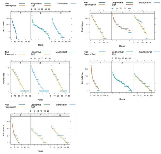
Figure 1.
Rank–abundance curves of floral species in the five agroecosystems (left up-) artificial forest, (right up) mixed horticulture and fruticulture, (left middle) native forest, (right middle) dairy prairies, and (left up) soybean per patch (1, 2, 3), with the abundance axis being in relative terms. In its construction, the range of the species (on the abscissa axis) and the percentage of accumulated abundance (on the ordinate axis) were used. The Vegan package (R) and radfit function were used.

Table 1.
The Apibotanical Interest Index (ABI) and the Agroecosystem Apibotanical Interest Index (AABI) from artificial forest (AF), dairy prairies (D), mixed horticulture and fruticulture (HF), soybean (S), and native forest (NF). Shannon–Wiener diversity index (ISH), number of species, flowering individuals, and Akaike information criterion (AIC) for each patch and agroecosystem.
Supplementary Material Figure S2 shows that agroecosystems AF, HF, D, and NF had asymptotic behavior from patch 2, indicating that the sampling efforts (number of patches sampled) were adequate. The S curve is not asymptotic, suggesting that the sampling effort was insufficient. A total of 46% of the species in the present study were included within the families with the most significant number of flowers in Uruguay []. On the other hand, 60% of the species with flowers belonged to six families. These were mentioned in melissopalynological and entomological studies as important honeybee flora and were present in all the agroecosystems (Supplementary Material Table S2). [,] documented that Asteraceae, Anacardiaceae, Rhamnaceae, Oxalidaceae, and Myrtaceae families highly depend on insect pollination. Moreover, the Myrtaceae family is considered one of the main families that provide resources, and, within this family, Eucalyptus sp. has significant beekeeping value [].
According to [], diversity indices are indicators of the distribution of abundance (or proportion) of species that occur in a territory. However, at the agroecosystem scale, the structure and the arrangement of individuals per species are important, not only the number. From a beekeeping point of view, when evaluating an agroecosystem, it is necessary to consider the availability of food resources for honeybees according to the distance from the hive [,].
Concerning the configuration of the agroecosystem, the presence of flowers was explained by the variable’s species richness, flowering period, seasonality over a year, and temperature conditions in the different agroecosystems (Supplementary Material Table S3). Temperature and seasonality showed significant differences among all agroecosystems (p value ≤ 0.005), except for AF (p value = 0.903). The agroecosystem that presented higher annual average temperatures was D (Supplementary Figure S1). Winter was the only season that did not show significant differences for the five agroecosystems (p value = 0.674). In winter, the average temperatures ranged from 10 to 15 °C, and few flowers were available (low presence) in any of the agroecosystems. The selected model showed significant differences for NF, AF, and HF regarding the species growth habit and flowering period. In these agroecosystems, trees and shrubs predominated, and, in agroecosystems D and S, the growth habit (GH) of solitary species thickets and stands predominated (Supplementary Material Table S4). These data show that the land uses where tree plantations and shrubs predominated had more flowers (high presence), providing food and shelter. In agreement with these results are the findings of te [,]. Furthermore [], stated that tree and shrub assemblies could guide foraging flights since they are more likely to orient bees better than open agricultural fields. Considering our results, the adoption of sustainable tree and shrub management practices surrounding apiaries’ areas of influence could favor future beekeeping scenarios at the agroecosystem scale.
3.2. Apibotanical Interest Index (ABI)
Table 1 shows the number of individuals in each agroecosystem. The results of the Shannon–Wiener diversity index (ISH) per patch and agroecosystem are also presented. This index was calculated because the location of the patches was random, and all species within each patch were present in the sample [].
The most significant number of individuals in AF, HF, and D were found in patch 1, while, in NF, it was patch 3 (Table 1). Supplementary Material Table S3 presents the independent variables that were included in the calculation of the ABI. The GLM was selected because it allowed using non-normal distributions of errors (such as binomials: presence or absence of blooms) and nonconstant variances.
The model was chosen from the 38 possibilities assayed based on the Akaike information criterion (AIC): the non-null model with the lowest AIC value. Within the models, a diversity of responses was found. This criterion measures the goodness of fit from the maximum likelihood of the model and its complexity through the number of parameters chosen. The results of each ABIi for each species are presented in Supplementary Material Table S4. The number of flowered individuals of each species was analyzed per patch, and their spatiotemporal functions were appraised. A quantitative-qualitative comparative value that integrated the heterogeneity of each agroecosystem and its function for beekeeping was calculated. It was possible to generate a list of apibotanical species where the same species obtained different ABIs due to its rating in each agroecosystem. Honeybees are more active in habitats with species diversity [], but the same floral species can be valued differently by bees depending on the ecosystem in which it is assembled.
3.3. Agroecosystem Apibotanical Interest Index (AABI) Development
From the results obtained from the AABI (Supplementary Material Table S4 and Table 1), a scale from one to five to interpret this index from an apicultural perspective was developed. The scores were 5 = prominent for honey harvest; 4 = moderate, which needs management for honey harvest; 3 = admissible agroecosystem, which presents difficulties for honey harvest without beekeepers’ permanent intervention; 2 = modest due to lack of flowering species, which limits honey production 1 = low considered insignificant for honey harvest. The agroecosystem that had outstanding apibotanical functionality was NF (AABI = 5), which was followed by the HF, AF, and D landscapes. We expected to find supplementary habitats when the patches in the agroecosystem were more heterogeneous, thus increasing the importance of biodiversity in the functioning of these agroecosystems. However, from a beekeeping point of view, these would require a greater energy expenditure from honeybees since they would have to travel more (time and distance) to replace species not present near the apiary. In this framework, according to Table 1 and Supplementary Material Figure S2, the agroecosystems that were considered supplementary with heterogeneous patches were AF and D with ISH values of 2.99 ± 0.36 and 3.31 ± 0.50, respectively, which had different ranges of dominance for the two patches within each agroecosystem. The patches with more homogeneous and complementary behavior were NF and HF with ISH values of 3.56 ± 0.001 and 3.37 ± 0.05 and with the same average dominant species in the three patches in each agroecosystem. For S, the data did not allow the inferring of conclusions.
According to Ref. [] Lázaro and Totland (2010), high floral diversity in a territory positively influences the permanence of the bees in the region. Pla (2006) established that the range of Shannon–Wiener diversity index (ISH) value is between 1 and 4.5 []. classified ISH values as follows: values lower than 1.5 are considered low, between 1.6 and 3 are medium, and equal to or greater than 3.1 are systems with high diversity. According to these authors, our results indicated the high diversity of the NF, HF, and D agroecosystems and medium diversity for AF (Table 1. The NF (without agriculture) site presented the most remarkable diversity, this could be a response to its location within a ravine, surrounded to the south and east by a plateau of native forests. Agricultural landscapes contain a lower diversity of resources for bee communities []. On the other hand, according to [], diversity indices are indicators of the species richness in a territory. Considering an agroecosystem as an association of plant covers within patches, represented by species with higher abundance, it was possible to evaluate their assemblies. This could be structured according to the distance from the hive and the availability of trophic resources for bee communities. The patches that showed higher ISH values were not selected as the representative ones of each agroecosystem. Instead, those patches with lower AIC presented the highest number of individuals and were better for beekeeping. For example, patch 1 in AF was the best representative of the agroecosystem (AIC 60.07), but its ISH was 2.37, being the lowest ISH of the three patches, while it had the highest number of individuals.
Agroecosystems with homogeneous structures, particularly natural forests, show that after a certain distance, no new species appear []. NF was the one that was best from a beekeeping point of view. The number of species between the patches differed only by four. Therefore, they were complementary habitats. Unlike the other agroecosystems, honeybees do not have to stray far from their hive looking for flowers. Ref. [] pointed out that the consequences of being eusocial insects are that workers feed mainly to help group members, and foraging efficiency may increase because individuals help each other to find feeding sites near the hive. The areas with a diversity of flowers near the nests compensate for the energy consumed when searching for food. According to our results, the NF and HF landscapes complied with this characterized, while D and AF would need higher energy expenditure due to the patch’s heterogeneity.
Our results showed that the agroecosystems with a higher ISH had a higher AABI (Table 1). In accordance with [,], the number of flowers over time and the presence of particularly attractive flowering species for bees are as important as diversity in the landscape. NF and HF were complementary habitats in composition and functional structure, while landscapes AF and D were supplementary habitats. The data indicated that the spatial–temporal diversity of the floral resources given by different land uses determined the availability of functional flowers for honeybees.
Furthermore, considering the composition of the flowers’ assemblage as a whole within an agroecosystem where bees feed and not a patchwork of different land uses permitted the standardization of the biodiversity of flower resources. According to Ref. [], honeybees only need a limited number of flowering plants to feed on.
Interestingly, the apiaries placed in landscapes where agriculture and artificial prairies were conducted produced very little honey in winter, if any (Figure 2). The native forest was the landscape with the highest AABI and was the most productive. Its biodiversity was a source of apibotanical species throughout the year. The lowest AABI score was obtained for apiaries in extensive soybean plantations. During the summer culturing season, honey production dropped. Still, after soybean was harvested in autumn, the biodiverse weeds served as the nectar source for bees, triggering honey production during spring before the first chemical tillage with glyphosate occurred. Eucalyptus flowers are intensively foraged by bees, so honey production was high in autumn even though this agroecosystem had low biodiversity. The apiaries in AF produced five to six times more honey during autumn than in any other season. A common practice is to move apiaries to Eucalyptus forests in autumn to improve honey yields. However, honey production during summer and spring was low in AF. The intermediate AABI value for the landscape explained the drop in productivity for these two seasons.
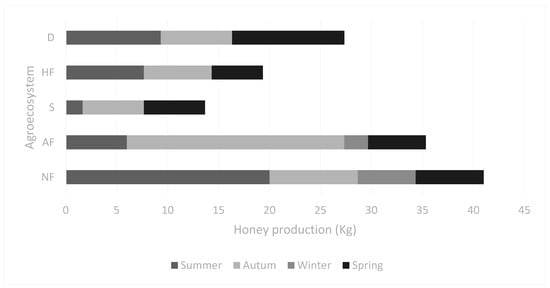
Figure 2.
Seasonal production of honey in the different landscapes. Agroecosystems: D: dairy prairies; AF: artificial Eucalyptus sp. forest; HF: mixed horticulture and fruticulture; S: soybean crop; NF: native forest.
It is necessary to clarify that if edaphoclimatic conditions change, these assemblages will change, and plant species that today complete the landscape may become functional species in the agroecosystems studied. It is worth mentioning that 34% of the species analyzed here were the flowers of spontaneous species threatened by chemical tillage management based on herbicide use. The point is critical for all agroecosystems with strong agricultural inputs. The disappearance of such resources would have a negative impact not only on bee survival but also on the quality of the beehive products collected from these environments [,,].
Plants and animals often respond to different environmental conditions (light, temperature, or their combination). Phenological mismatches driven by global temperature increases may have consequences for the plant and animal species that depend on each other for reproductive success, such as outcrossing plants and their pollinators []. The vegetative tissues of plants respond rapidly to changes in the surrounding environment: leaves and cotyledons often elongate in response to increased temperature [], and lateral root emergence has been observed in plants exposed to drought []. In contrast, to ensure metabolic resilience and the completion of gamete and embryo development, flowers are equipped with a battery of functionally redundant sugar and amino acid transporters []. However, the observation that the yield of many crops is markedly reduced when heat, cold, and drought occur during the flowering season (FAO, Food and Agriculture Organization of the United Nations https://www.fao.org, accessed on 4 February 2024) is an indication that flowers are more vulnerable than vegetative tissues to abiotic stresses [,].
Within this framework, the results presented here may be overestimated for agricultural ecosystems such as annual crops (prairies, soybean). In agreement with [], the flowers produced in large quantities of commercial farm crops to attract pollinators may be affected by the thermal differences that occur between the day and night. This means that nectar secretion may not occur, for example, due to low root development with unfavorable climatic conditions (low temperatures and abundant rainfall). Herbaceous species depend on night temperatures and root development to absorb water, which is translocated it to the nectaries to attract pollinators through nectar secretion. Therefore, the attractiveness of a herbaceous plant (GH = 2) with a high ABI (greater than three) predominating in the prairies, for example, in agroecosystem D, may be overestimated. For this reason, even if flowers are present, the hives sometimes have no honey. The agroecosystems that could have been underestimated in this study were NF, HF, and AF, in which trees and shrubs predominated (GH = 4 and GH = 5). These are nonherbaceous species with a reserve cambium (trunk). They are better adapted and not as dependent on climatic conditions. Therefore, they always have nectar secretions that can be collected by bees. In NF, for example, individuals of the same species bloom at different times throughout a season, while crops are more homogeneous, with shorter flowering and nectar secretion periods.
Agroecosystem management is fundamentally important in agricultural landscapes such as HF, S, D, and AF. The less-impacted landscapes, such as NF, without intensive agriculture, had complementary assemblages; they presented a higher diversity index, and the plots were homogeneous at increasing distances from the apiary. In these cases, their blooms complemented each other. Interestingly, the HF agroecosystem had the same behavior. The high diversity of cultured species, which are most highly attractive to bees, and the crop variation throughout the year could be the explanation (Supplementary Material Figure S1).
4. Conclusions
The sole occurrence of melliferous botanical species with a high ABI is insufficient to evaluate a landscape’s usefulness for honey production properly. It depends on the species’ assemblage, which we proposed to be qualified with the AABI. Bees can use the same species differently depending on the assemblage of the agroecosystem.
The AABI presented in this work, based on assembly rules and expected attributes for beekeeping, constitutes a tool for generating scenarios that allow alleviating the unpredictable effects of changes in landscapes, whether due to climate change or agriculture, and improving honey productivity.
Supplementary Materials
The following supporting information can be downloaded at https://www.mdpi.com/article/10.3390/ecologies6010003/s1, Figure S1: Average rainfall in millimeters (top) and temperatures in degrees Celsius (bottom) for the five agroecosystems for (A) autumn, (SM) summer (SP) spring, and (W) winter; Figure S2: Species accumulation curve (y-axis) as a function of sampling patches (1, 2, and 3) (x-axis) (Rstudio, Library Vegan). The results of the floral species accumulation curves per sampling patch in native forest, soybean, dairy prairies, mixed horticulture and fruticulture, and artificial forest agroecosystem are presented. Table S1: Georeferenced and characterizations of each agroecosystem’s land use; Table S2: Flowering family and species list according to references found for each pollen species in convertible (C) and support honey (So): 5 = frequency classes with dominant pollen (>45%) and secondary pollen (15–45%); 3 = minor pollen importance (13–15%) and trace pollen (<3%); 1 = not found; Table S3. ANOVA of the Generalized Linear Model (GLM) using maximum significance as partition criterion. Independent variables: P: flowering period, SR: species richness, SS: growth habit, Seasonality (summer, autumn, spring and winter), TT: temperature, and US: land use (native forest, artificial forest, dairy, soybean, mixed horticulture and fruticulture). Presented results of a model with better significance or with a strong trend (Number of Fisher Scoring iterations: 5 (of the 38 models proposed) including the different explanatory variables at the landscape scale. Call: glm(formula = cbind(Flo) ~ P * SR + P+ SR + SS + US + US * TT + Seasonality, family = binomial(link = logit)). Signify. Codes: 0 ‘***’ 0.001 ‘**’ 0.01 ‘*’ 0.05 ‘.’ 0.1 ‘ ’ 1,(Dispersion parameter for binomial family taken to be 1) Null deviance: 2236.3 on 2278 degrees of freedom, Residual deviance: 1182.5 on 2262 degrees of freedom; AIC: 1216.5; Table S4: Results of ABI for each agroecosystem per family, species, and growth habit (GH). A = artificial forest; HF = mixed horticulture and fruticulture; NF = native forest; S = soybean and D = dairy prairies. GH scale: 5 = trees; 4 = bush; 3 = stand; 2 = thicket; 1 = stem. ABI scale: 5 = prominent for honey harvest; 4 = moderate, which needs management for honey harvest; 3 = admissible, which presents difficulties for honey harvest without beekeepers’ permanent intervention; 2 = modest due to lack of bloom; 1 = low, considered insignificant for honey harvest. References [,,,,,,,,,,,,,,,,,,,,,,,,,,] are cited in the Supplementary Materials.
Author Contributions
Conceptualization, R.D., S.N., M.V.C. and H.H.; methodology, R.D., S.N. and H.H.; software, R.D.; validation, R.D., S.N. and H.H.; formal analysis, R.D.; investigation, R.D., S.N., M.V.C. and H.H.; resources, R.D., S.N., M.V.C. and H.H.; data curation, R.D., S.N. and H.H.; writing—original draft preparation, R.D., S.N. and H.H.; writing—review and editing, R.D., S.N., M.V.C. and H.H.; visualization, R.D.; supervision, S.N. and H.H.; project administration, S.N. and M.V.C.; funding acquisition, R.D., S.N., M.V.C. and H.H. All authors have read and agreed to the published version of the manuscript.
Funding
This work was supported by the National Institute of Agricultural Research project FPTA 320 and ANII- Fondo Maria Vinas, FMV_1_2023_1_176173.
Institutional Review Board Statement
Not applicable.
Informed Consent Statement
Not applicable.
Data Availability Statement
Data is available in the article and Supplementary Materials.
Conflicts of Interest
The authors declare no conflicts of interest.
References
- Tscharntke, T.; Steffan-Dewenter, I.; Kruess, A.; Thies, C. Characteristics of insect populations on habitat fragments: A mini review. Ecol. Res. 2002, 17, 229–239. [Google Scholar] [CrossRef]
- Fischer, J.; Lindenmayer, D.B.; Manning, A.D. Biodiversity, ecosystem function, and resilience: Ten guiding principles for commodity production landscapes. Front. Ecol. Environ. 2006, 4, 80–86. [Google Scholar] [CrossRef]
- Seeley, T. The Wisdom of the Hive: The Social Physiology of Honeybee Colonies; Harvard Press: Cambridge, MA, USA, 1995. [Google Scholar]
- Steffan-Dewenter, I.; Münzenberg, U.; Bürger, C.; Thies, C.; Tscharntke, T. Scale dependent. Effects of landscape context on three pollinator guilds. Ecology 2002, 83, 1421–1432. [Google Scholar] [CrossRef]
- Garbuzov, M.; Couvillon, M.; Schürch, R.; Ratnieks, F. Honey bee dance decoding and pollen-load analysis show limited foraging on spring-flowering oilseed rape, a potential source of neonicotinoid contamination. Agric. Ecosyst. Environ. 2015, 203, 62–68. [Google Scholar] [CrossRef]
- Danner, N.; Molitor, A.M.; Schiele, S.; Härtel, S.; Steffan-Dewenter, I. Season and landscape composition affect pollen foraging distances and habitat use of honey bees. Ecol. Appl. 2016, 26, 1920–1929. [Google Scholar] [CrossRef] [PubMed]
- Hemberger, J.; Witynski, G.; Gratton, C. Floral resource continuity boosts bumble bee colony performance relative to variable floral resources. Ecol. Entomol. 2022, 47, 703–712. [Google Scholar] [CrossRef]
- Timberlake, T.P.; Vaughan, I.P.; Baude, M.; Memmott, J. Bumblebee colony density on farmland is influenced by late-summer nectar supply and garden cover. J. Appl. Ecol. 2021, 58, 1006–1016. [Google Scholar] [CrossRef]
- Scheper, J.; Bommarco, R.; Holzschuh, A.; Potts, S.G.; Riedinger, V.; Roberts, S.P.; Rundlöf, M.; Smith, H.G.; Steffan-Dewenter, I.; Wickens, J.B.; et al. Local and landscape-level floral resources explain effects of wildflower strips on wild bees across four European countries. J. Appl. Ecol. 2015, 52, 1165–1175. [Google Scholar] [CrossRef]
- Cole, L.J.; Brocklehurst, S.; Robertson, D.; Harrison, W.; McCracken, D.I. Exploring the interactions between resource availability and the utilization of semi-natural habitats by insect pollinators in an intensive agricultural landscape. Agric. Ecosyst. Environ. 2017, 246, 157–167. [Google Scholar] [CrossRef]
- Maurer, C.; Sutter, L.; Martínez-Núñez, C.; Pellissier, L.; Albrecht, M. Different types of semi-natural habitat are required to sustain diverse wild bee communities across agricultural landscapes. J. Appl. Ecol. 2022, 59, 2604–2615. [Google Scholar] [CrossRef]
- Taki, H.; Kevan, P.G.; Viana, B.F.; Silva, O.F.; Buck, M. Artificial covering on trap nests improves the colonization of trap-nesting wasps. J. Appl. Ecol. 2007, 132, 225–229. [Google Scholar] [CrossRef]
- Tscharntke, T.; Brandl, R. Plant-insect interactions in fragmented landscapes. Annu. Rev. Entomol. 2004, 49, 405–430. [Google Scholar] [CrossRef]
- Van de Koppel, J.; Bardgett, R.D.; Bengtsson, J.; Rodriguez-Barrueco, C.; Rietkerk, M.; Wassen, J.; Wolters, V. The effects of spatial scale on trophic interactions. Ecosystems 2005, 8, 801–807. [Google Scholar] [CrossRef][Green Version]
- Dunning, J.B.; Danielson, B.J.; Polliam, H.R. Ecological processes that affect populations in complex landscapes. Oikos 1992, 65, 169–175. [Google Scholar] [CrossRef]
- Westrich, P. Habitat requirements of central european bees and the problems of partial habitats. In The Conservation of Bees; Matheson, A., Buchmann, S.L., O’Toole, C., Westrich, P., Williams, I., Eds.; Academic Press: London, UK, 1996; pp. 1–6. [Google Scholar]
- Díaz, R.; Niell, S.; Cesio, M.V.; Heinzen, H. Floral food resources for Apis mellifera (Hymenoptera: Apidae) in a mountain forest area in Uruguay. Agrociencia Urug. 2021, 25, e426. [Google Scholar] [CrossRef]
- Harris, C.; Balfour, N.J.; Ratnieks, F.L. Seasonal variation in the general availability of floral resources for pollinators in northwest Europe: A review of the data. Biol. Conserv. 2024, 298, 110774. [Google Scholar] [CrossRef]
- Garbuzov, M.; Balfour, N.J.; Shackleton, K.; Al Toufailia, H.; Scandian, L.; Ratnieks, F.L. Multiple methods of assessing nectar foraging conditions indicate peak foraging difficulty in late season. Insect. Conserv. Divers. 2020, 13, 532–542. [Google Scholar] [CrossRef]
- Sponsler, D.; Dominik, C.; Biegerl, C.; Honchar, H.; Schweiger, O.; Steffan-Dewenter, I. High rates of nectar depletion in summer grasslands indicate competitive conditions for pollinators. Oikos 2024, 2024, e10495. [Google Scholar] [CrossRef]
- Meikle, W.G.; Rector, B.G.; Mercadier, G.; Holst, N. Within-day variation in continuous hive weight data as a measure of honey bee colony activity. Apidologie 2008, 39, 694–707. [Google Scholar] [CrossRef]
- Timberlake, T.P.; Vaughan, I.P.; Memmott, J. Phenology of farmland floral resources reveals seasonal gaps in nectar availability for bumblebees. J. Appl. Ecol. 2019, 56, 1585–1596. [Google Scholar] [CrossRef]
- Cesio, V.; Niell, S.; Díaz, R.; Jesús, F.; Gérez, N.; Santos, E.; Heinzen, H.; Franco, J.; Notte, G.; Cancela, H. Estudio de la Distribución de Residuos de Agroquímicos en Productos de la Colmena y su Relación Con Las Zonas de Producción Apícola del País. FPTA INIA Nº 2020; Volume 89, p. 34. Available online: https://inia.uy/sites/default/files/publications/2024-10/Inia-Fpta-89-proyecto-320-2020.pdf (accessed on 1 November 2024).
- Braun-Blanquet, J. Fitosociología. Bases Para el Estudio de las Comunidades Vegetales; Blume: Madrid, Spain, 1979; 820p. [Google Scholar]
- Dengler, J. Phytosociology. Int. Encycl. Geogr. People Earth Environ. Technol. 2016, 12, 1–6. [Google Scholar] [CrossRef]
- Delaplane, K.; Van der Steen, J.; Guzman, E. Standard methods for estimating strength parameters of Apis mellifera colonies. J. Apic. Res. 2013, 52, 5–7. [Google Scholar] [CrossRef]
- Core Team R. Core Team R: A Language and Environment for Statistical Computing, R Development V4.4.1.; R Foundation for Statistical Computing: Vienna, Austria, 2005.
- Buddle, C.M.; Beguin, J.; Bolduc, E.; Mercado, A.; Sackett, T.E.; Selby, D.R.; Varady-Burgos, M.G.; Sánchez, A.C. Preferencias alimenticias en las mieles inmaduras de Apis mellifera en el Chaco Serrano (Jujuy, Argentina). Bol. Soc. Argent. Bot. 2014, 49, 41–50. [Google Scholar]
- Lambshead, P.J.D.; Platt, H.M.; Shaw, K.M. The detection of differences among assemblages of marine benthic species based on an assessment of dominance and diversity. J. Nat. Hist. 1983, 17, 859–874. [Google Scholar] [CrossRef]
- Akaike, H. A new look at the statistical model identification. IEEE Trans. Autom. Control 1974, 19, 716–723. [Google Scholar] [CrossRef]
- Matteucci, S.D. La cuestión del patrón y la escala en la ecología del paisaje. In Sistemas Ambientales Complejos: Herramientas de Análisis Espacial; Matteucci, S.D., Buzai, G.D., Eds.; EUDEBA: Buenos Aires, Argentina, 1998; pp. 219–248. [Google Scholar]
- Magurran, A. Measuring Biological Diversity; Blackwell Publishing: Malden, MA, USA, 2004; 70p. [Google Scholar]
- Brussa, C.; Grela, I. Flora Arbórea del Uruguay. In Con Énfasis en Las Especies de Rivera y Tacuarembó; COFUSA: Montevideo, Uruguay, 2007; p. 544. ISBN 9974963346. [Google Scholar]
- Crane, E. The plant resources of honeybee. Apiacta 1991, 26, 57–64. [Google Scholar]
- Andrada, A.C. Flora utilizada por Apis mellifera L. en el sur del Caldenal (Provincia Fitogeográfica del Espinal) Argentina. Rev. Mus. Argent. Cienc. Nat. 2003, 5, 329–336. [Google Scholar] [CrossRef]
- Basilio, A.M. Cosecha polínica por Apis mellifera (Hymenoptera) en el bajo Delta del Paraná: Comportamiento de las abejas y diversidad del polen. Rev. Mus. Argent. Cienc. Nat. 2000, 2, 111–121. [Google Scholar] [CrossRef][Green Version]
- Ugland, K.I.; Gray, J.S.; Ellingsen, K.E. The species–accumulation curve and estimation of species richness. J. Anim. Ecol. 2003, 72, 888–897. [Google Scholar] [CrossRef]
- Loreau, M.; Mouquet, N.; Holt, R.D. Meta-ecosystems: A theoretical framework for a spatial ecosystem ecology. Ecol. Lett. 2003, 6, 673–679. [Google Scholar] [CrossRef]
- Dimitrakopoulos, P.G.; Schmid, B. Biodiversity effects increase linearly with biotope space. Ecol. Lett. 2004, 7, 574–583. [Google Scholar] [CrossRef]
- Tellería, M.C. Palynological analysis of food reserves found in a nest of Bombus atratus (Hym. Apidae). Grana 1998, 37, 125–127. [Google Scholar] [CrossRef]
- Abrahamovich, A.; Tellería, M.C.; Díaz, N.B. Bombus species and their associated flora in Argentina. Bee World 2001, 82, 60–75. [Google Scholar] [CrossRef]
- Cranmer, M.J.; McCollin, L.; Ollerton, J. Landscape structure influences pollinator movements and directly affects plant reproductive success. Oikos 2012, 121, 562–568. [Google Scholar] [CrossRef]
- Mostacedo, B.; Fredericksen, T. Manual de Métodos Básicos de Muestreo y Análisis en Ecología Vegetal; Proyecto de Manejo Froestal Sostenible (BOLFOR): Santa Cruz, Bolivia, 2000; Volume 87, pp. 1–92. Available online: http://www.bio-nica.info/Biblioteca/Mostacedo2000EcologiaVegetal.pdf (accessed on 1 November 2024).
- Potts, S.; Vulliamy, B.; Dafni, A.; Ne’eman, G.; Willmer, P. Linking bees and flowers: How do floral communities structure pollinator communities? Ecology 2010, 84, 2628–2642. [Google Scholar] [CrossRef]
- Lázaro, A.; Totland, O. Local floral composition and the behavior of pollinators: Attraction to foraging within experimental patches. Ecol. Entomol. 2010, 35, 652–661. [Google Scholar] [CrossRef]
- Roulston, T.H.; Karen, G. The role of resources and risks in regulating wild bee populations. Annu. Rev. Entomol. 2011, 56, 293–312. [Google Scholar] [CrossRef] [PubMed]
- Pla, L. Biodiversidad: Inferencia basada en el índice de Shannon y la riqueza. Interciencia 2006, 31, 583–590. [Google Scholar]
- Beekman, M.; Ratnieks, W. Long-range foraging by the honeybee, Apis mellifera. Funct. Ecol. British Ecol. Soc. 2001, 14, 490–496. [Google Scholar] [CrossRef]
- Tylianakis, J.; Rand, T.; Kahmen, A.; Klein, A.; Buchmann, N.; Perner, J.; Tscharnktke, T. Resource Heterogeneity Moderates the Biodiversity-Function Relationship in Real World Ecosystems. PLoS Biol. 2008, 6, e122. [Google Scholar] [CrossRef]
- Jha, S.; Kremen, C. Resource diversity and landscape -level homogeneity drive native bee foraging. Proc. Natl. Acad. Sci. USA 2013, 110, 555–558. [Google Scholar] [CrossRef] [PubMed]
- Goulson, D.; Nicholls, E.; Botías, C.; Rotheray, E.L. Bee declines driven by combined stress from parasites, pesticides, and lack of flowers. Science 2015, 347, 1255957. [Google Scholar] [CrossRef] [PubMed]
- Kremen, C.; Mc Gonigle, L.K. Small-scale restoration in intensive agricultural landscapes supports more specialized and less mobile pollinator species. J. Appl. Ecol. 2015, 52, 602–610. [Google Scholar] [CrossRef]
- Ekroos, J.; Ödman, A.M.; Andersson, G.K.; Birkhofer, K.; Herbertsson, L.; Klatt, B.K.; Rundlöf, M. Sparing land for biodiversity at multiple spatial scales. Front. Ecol. Evol. 2016, 3, 145. [Google Scholar] [CrossRef]
- Ovaskainen, O.; Skorokhodova, S.; Yakovleva, M.; Sukhov, A.; Kutenkov, A.; Kutenkova, N.; Shcherbakov, A.; Meyke, E.; Delgado, M.d.M. Respuesta fenológica a nivel comunitario al cambio climático. Actas Acad. Nac. Cienc. EE UU 2013, 110, 13434–13439. [Google Scholar]
- Quint, M.; Delker, C.; Franklin, K.A.; Wigge, P.A.; Halliday, K.J.; van Zanten, M. Control molecular y genético de la termomorfogénesis de las plantas. Nat. Plants 2016, 2, 15190. [Google Scholar] [CrossRef] [PubMed]
- Babé, A.; Lavigne, T.; Séverin, J.P.; Nagel, K.A.; Walter, A.; Chaumont, F.; Batoko, H.; Beeckman, T.; Draye, X. Repression of early lateral root initiation events by transient water deficit in barley and maize. Philos. Trans. R. Soc. Lond. B Biol. Sci. 2011, 367, 1534–1541. [Google Scholar] [CrossRef] [PubMed] [PubMed Central]
- Borghi, M.; Fernie, A.R. Floral Metabolism of Sugars and Amino Acids: Implications for Pollinators’ Preferences and Seed and Fruit Set. Plant Physiol. 2017, 175, 1510–1524. [Google Scholar] [CrossRef] [PubMed]
- Barnabas, B.; Jager, K.; Feher, A. The effect of drought and heat stress on reproductive processes in cereals. Plant Cell Environ. 2008, 31, 11–38. [Google Scholar] [CrossRef]
- Prasad, P.V.; Djanaguiraman, M.; Perumal, R.; Ciampitti, I.A. Impact of high temperature stress on floret fertility and individual grain weight of grain sorghum: Sensitive stages and thresholds for temperature and duration. Front. Plant Sci. 2015, 6, 820. [Google Scholar] [CrossRef]
- Achkar, M.; Domínguez, A.; Pesce, F. Los Recursos Naturales en el Actual Modelo de Desarrollo. Poster Central: Ecorregiones del Uruguay; Revista de la Educación del Pueblo: Montevideo, Uruguay, 2012; p. 92. [Google Scholar]
- Fagúndez, G.; Reinoso, D.; Aceñolaza, P. Caracterización y fenología de especies de interés apícola en el departamento Diamante (Entre Ríos, Argentina). Boletín Soc. Argent. Botánica 2016, 51, 243–267. [Google Scholar] [CrossRef]
- Basilio, A.M.; Romero, E.J. Variaciones anuales y estacionales en el contenido polínico de la miel de un colmenar RIA. Rev. Investig. Agropecu. 2002, 31, 41–58. Available online: https://www.redalyc.org/articulo.oa?id=86431103 (accessed on 4 February 2024).
- Granados-Argüello, R.; Villanueva-Gutiérrez, R.; Martínez-Hernández, E.; García Mayoral, L.; González de la Torre, J. Análisis melisopalinológico de mieles de Apis mellifera en la zona centro de Veracruz, México. Polibotanica 2020, 50, 147–163. [Google Scholar] [CrossRef]
- Miranda, D.E.; Molina, R.A.; Aquino, D.Y.; Pellizzer, N.A.; Berdún, A.; Fernández, L.C.; Huk, L.H. Flora utilizada por Apis mellifera L. y Tetragonisca fiebrigi Schwarz en 5 departamentos de la zona centro-norte de la Provincia de Misiones, Argentina. Yvyraretá: Rev. For. País Árboles. Eldorado (Misiones) UNaM. FCF 2018, 26, 38–54. Available online: https://rid.unam.edu.ar/handle/20.500.12219/2638?show=full (accessed on 1 November 2024).
- Salgado, C.R.G.; Piesko, G.; Tellería, M.C. Aporte de la melisopalinología al conocimiento de la flora melífera de un sector de la Provincia Fitogeográfica Chaqueña. Bol. Soc. Argent. Bot. 2014, 49, 513–524. [Google Scholar] [CrossRef]
- Reyes, N.J.; Asesor, P.N.; Albarracín, V.N.; García, M.E.; Espeche, M.L. Caracterización palinológica de la miel de un sector de la región chaqueña de la provincia de Tucumán (Argentina). Bol. Soc. Argent. Bot. 2019, 54, 367–379. [Google Scholar] [CrossRef]
- Gutiérrez, P.B.; Quiroz, D.L. Estudio melisopalinológico de dos mieles de la porción sur del valle de México. Polibotánica 2007, 23, 57–75. Available online: https://www.redalyc.org/pdf/621/62102304.pdf (accessed on 1 November 2024).
- Madanes, N.; Millones, A. Estudio del polen aéreo y su relación con la vegetación en un agroecosistema. Darwiniana 2004, 42, 51–62. [Google Scholar]
- Tellería, M.C.; Salgado, C.; Andrada, C. Rhamnaceae asociada a mieles fétidas en Argentina. Rev. Mus. Argent Cienc. Nat. 2006, 8, 237–241. [Google Scholar]
- Costa, M.C.; Vergara-Roig, V.A.; Kivatinitz, S. A melissopalynological study of artisanal honey produced in Catamarca (Argentina). Grana 2013, 52, 9–37. [Google Scholar] [CrossRef]
- Cabrera, M.M. Identidad de Las Mieles de la Región Nordeste del Distrito Oriental del Parque Chaqueño. Doctoral Thesis, Universidad Nacional del Nordeste, Facultad de Ciencias Agrarias, Corrientes, Argentina, 2021. Available online: http://repositorio.unne.edu.ar/handle/123456789/29641 (accessed on 1 November 2024).
- Daners, G.; Tellería, C. Native vs. introduced bee flora: A palynological survey of honeys from Uruguay. J. Apic. Res. 1998, 37, 221–229. Available online: https://www.researchgate.net/publication/323773206_Uruguay_Daners_Telleria_Journal_Apic_Res_1998 (accessed on 1 November 2024). [CrossRef]
- Méndez, M.; Sánchez, A.; Flores, F.; Lupo, L. Análisis polínico de mieles inmaduras en el sector oeste de las yungas de Jujuy (Argentina). Bol. Soc. Argent. Bot. 2016, 51, 449–462. [Google Scholar] [CrossRef]
- Fagúndez, G.A. Estudio de Los Recursos Nectaríferos y Poliníferos Utilizados Por Apis mellifera L. en Diferentes Ecosistemas del Departamento Diamante (Entre Ríos). Doctoral Thesis, UNS. Bahía Blanca, Provincia de Buenos Aires, Argentina, 2011. Available online: https://repositoriodigital.uns.edu.ar/handle/123456789/500 (accessed on 1 November 2024).
- Valtierra, M.; Bonifacino, J. Revisión taxonómica de Baccharis Sect. Heterothalamus (Less.) (Asteraceae: Asterae) en Uruguay. Boletín Soc. Argent. Botánica 2014, 49, 613–620. [Google Scholar] [CrossRef][Green Version]
- Basilio, A.M.; Romero, E.J. Contenido polínico en las mieles de la región del Delta del Paraná (Argentina). Darwiniana 1996, 34, 113–120. Available online: https://www.ojs.darwin.edu.ar/index.php/darwiniana/article/view/384 (accessed on 1 November 2024).
- Basilio, A.M. Estudio Melitopalinológico de Los Recursos Alimentarios y de la Producción de un Colmenar en la Región del Delta del Paraná, Argentina. Doctoral Dissertation, Universidad de Buenos Aires. Facultad de Ciencias Exactas y Naturales, Buenos Aires, Argentina, 1992. Available online: https://hdl.handle.net/20.500.12110/tesis_n3012_Basilio (accessed on 1 November 2024).
- Bazurro, D.; Díaz, R.; Sánchez, M. Tipificación de miel de Palma Butiá (Butia capitata) Durante la Floración de 1995–1996 en el Departamento de Rocha. Rocha: Universidad de la República. Documentos de Trabajo: 12, 1997, 29page. Available online: https://www.probides.org.uy/imagenes/ckfinder/files/files/Documentos%20de%20Trabajo/DT12.pdf (accessed on 1 November 2024).
- Alaniz-Gutiérrez, L.; Ail-Catzim, C.E.; Villanueva-Gutiérrez, R.; Delgadillo-Rodríguez, J.; Ortiz-Acosta, M.E.; García-Moya, E.; Medina Cervantes, T.S. Caracterización palinologica de las mieles del Valle de Mexicali, Baja California, México. Polibotánica 2017, 43, 257–285. [Google Scholar]
- Flores, F.; Sánchez, A. Primeros resultados de caracterización botánica de mieles de tetragonisca angustula Latreille (Apidae, Meliponinae) criadas en la localidad Los Naranjos-Orán–Salta. Bol. Soc. Argent. Bot. 2010, 45, 81–91. [Google Scholar]
- Perez de Zabalza, A. Análisis polínico de mieles de los valles pirenaicos navarros (España). In Actes del Simposi Internacional de Botànica “Pius Font i Quer” Vol. II Fanerogàmia; Institut d’Estudis Ilerdencs: Lleida, Spain, 1992; pp. 183–187. Available online: https://hdl.handle.net/10171/27665 (accessed on 1 November 2024).
- Hidalgo, M.I.; Cabezudo, B. Producción de néctar en matorrales del Sur de España. Acta Botánica Malacit. 1995, 20, 123–132. [Google Scholar] [CrossRef]
- Corbella, E.; Tejera, L.; Cernuschi, F. Calidad y origen botánico de mieles del noreste de Uruguay. Rev. INIA 2005, 3, 6–7. Available online: http://www.ainfo.inia.uy/digital/bitstream/item/215/1/111219220807150246.pdf (accessed on 1 November 2024).
- Basilio, A. Polen de las especies hidrófitas en las mieles del delta del Río Paraná (Argentina). Bol. Soc. Argent. Bot. 1996, 31, 231–234. Available online: https://botanicaargentina.org.ar/wp-content/uploads/2018/08/231-234011.pdf (accessed on 1 November 2024).
- Jato, M.V.; Iglesias, M.I.; Rodríguez-Gracia, V. A contribution to the environmental relationship of the pollen spectra of honeys from Ourense (NW Spain). Grana 1994, 33, 260–267. [Google Scholar] [CrossRef]
- Paredes, A.M.; Sosa, R.; Valdez, E.; Surkan, S. Evaluación diagnostica de mieles de distintas zonas apícolas de Misiones VI. Jorn. Científico Tecnológicas 2007, 317–320. Available online: www.alimentosargentinos.gob.ar (accessed on 1 November 2024).
Disclaimer/Publisher’s Note: The statements, opinions and data contained in all publications are solely those of the individual author(s) and contributor(s) and not of MDPI and/or the editor(s). MDPI and/or the editor(s) disclaim responsibility for any injury to people or property resulting from any ideas, methods, instructions or products referred to in the content. |
© 2024 by the authors. Licensee MDPI, Basel, Switzerland. This article is an open access article distributed under the terms and conditions of the Creative Commons Attribution (CC BY) license (https://creativecommons.org/licenses/by/4.0/).