Proceeding Paper

A Regression Line for a Laser Doppler Anemometer †

by
Karolina Weremijewicz
1 and
Andrzej Gajewski
2,*
1
Students’ Scientific Society “Heat Engineer”, Bialystok University of Technology, Wiejska Street 45 A, 15-351 Białystok, Poland
2
Department of HVAC, Bialystok University of Technology, Wiejska Street 45 A, 15-351 Białystok, Poland
*
Author to whom correspondence should be addressed.
Presented at Innovations-Sustainability-Modernity-Openness Conference (ISMO’21), Bialystok, Poland, 14 May 2021.
Environ. Sci. Proc. 2021, 9(1), 12; https://doi.org/10.3390/environsciproc2021009012
Published: 21 October 2021
(This article belongs to the Proceedings of Innovations-Sustainability-Modernity-Openness Conference (ISMO’21))

Abstract

:
Refrigeration and air conditioning consume 15% of the total generated electricity. Vapor condensation devices need a heat sink which may come in the form of absorption cycles devices. Two fluids, which change phase and concentration, flow through these devices. These changes take place amid a two-phase flow in contact with a solid phase. Hence, an extended study of the velocity profiles across the thin liquid layer is necessary, which is assumed to be conducted by a laser Doppler anemometer. The preliminary studies concerning the calibration of this anemometer are reported.

1. Introduction

The International Institute of Refrigeration in Paris estimated that 15% of the global electrical energy production is supplied to refrigeration and air conditioning systems; the latter consume about 45% of the energy in households and commercial buildings. However, driving the traditional vapor compression devices needs electricity generated in a thermal power station, which depletes limited fuel resources [1]. A limitation of electrical energy usage enables the absorption cycle devices whose electricity demands are less than 5% of the cooling capacity. These devices may utilize energy from renewable resources or wasted energy with a temperature of at least 80 °C [2]; their main weakness is a great volume in relation to the cooling capacity [3]. These systems consist of the devices through which two fluid substances flow in different phases and concentrations [4]. In order te the most effective, phase and concentration changes need a thin liquid film covering all of the exchange surface. Hence, the process of a film break up into the rivulets is the subject of the investigations that needs acquaintance with the velocity profile; the simplest formula of this profile was derived by Nusselt (1916) (cf. Madejski [5]) as a one dimensional function. Hartley and Murgatroyd [6] discussed two stability criteria: a force balance in the stagnation point and a thermodynamic equilibrium. Bankoff [7] presumed both discharge mass and the sum of the kinetic and surface energies in the liquid film were equal to these in the rivulets. Mikielewicz and Moszyński [8], [9] included in their analysis, the surface energy of the solid-gas phase. Two dimensional velocity profiles for a rivulet on a vertical surface were obtained by El-Genk and Saber [10], as well as by Perazzo and Gratton [11], while Tanasijczuk et al. [12] received a profile for a rivulet hanging from a horizontal plane. Ataki and Bart [13] used the Nusselt profile in the analysis of their experiments. Charogiannis et al. [14] experimentally determined the laminar velocity profile for a Reynolds number (Re) of less than 5.9 and a Kapitza number (Ka) of 14; they also obtained the average velocity profiles for the wavy flow of Re ≈ 5.2, with a forcing frequency between 2 and 6 Hz, as well as for Re = 25 and Re = 27, Ka = 85, with the frequencies 7 and 10 Hz.
The main area of research was the experimental determination of velocity profile in thin liquid layers for a wide range of Reynolds numbers with a laser Doppler anemometer (LDA) used as a measuring device. For this reason a calibration of LDA system was necessary and was the subject of the study.

2. Methodology

The experiments are conducted using a system of apparatus [15]. Figure 1 shows the laser beams (1) intersecting in the cross-section with a fully developed flow. They are generated by the laser Doppler anemometer (5) and directed through an optical fiber (3) to the optical system (2) moved to the desired positions by the optical benches system (8) regulated by the controller (6). These devices are controlled by a piece of software installed on the microcomputer (9) and run by a researcher who also fixes the desired flow rates by using the valve (19) and the float meter (20). A stable flow is maintained by the constant height difference between the water levels in the tanks (12) and (21).
A benchmark is a laminar flow whose velocity profile is measured 30 times at 31 points across the tube, ∅30 mm (15). The fixed errors δfixed(ri), which are the differences between a laminar velocity v l ( r i ) in a point at the radius ri and a mean velocity v ¯ L D A ( r i ) from a set of 30 measurements made by the LDA system in this point, and the standard deviation σ for the arithmetic mean, v ¯ L D A ( r i ) are determined as follows:
δ f i x e d ( r i ) = v l ( r i ) v ¯ L D A ( r i ) ,
σ ( r i ) = 1 30 ( j = 1 30 ( v ¯ L D A ( r i ) v L D A j ( r i ) ) 2 ) 1 / 2 .
Next the overall errors δoverall(ri) are computed as the square root of the sum of the squares of the fixed error and doubled standard deviation [16]; their inverse squares are the weights wi:
w i = 1 ( δ o v e r a l l ( r i ) ) 2 = 1 ( δ f i x e d ( r i ) ) 2 + ( 2 σ ( r i ) ) 2 .
Finally, a weighted regression line slope a and a Pearson’s correlation coefficient rxy are obtained [17]:
a = w i v ¯ L D A ( r i ) v l ( r i ) w i [ v ¯ L D A ( r i ) ] 2 ,
r x y = w i v ¯ L D A ( r i ) v l ( r i ) { w i [ v ¯ L D A ( r i ) ] 2 w i [ v l a m ( r i ) ] 2 } 1 / 2 .

3. Results and Discussion

The regression line is computed from Equation (4) and the experimental results are plotted in Figure 2 where the regression equation and Pearson’s correlation coefficient value are also recorded.
Since the slope of the function is close to 1 and the Pearson’s correlation coefficient value is much higher, then its critical value equals 0.3557 for 29 degrees of freedom at a 95% confidence level and it may be concluded the applied system of apparatus maintains a high measurement quality.

Author Contributions

A.G. conceived and designed the experiments; K.W. and A.G. performed the experiments; K.W. and A.G. analyzed the data; A.G. and K.W. wrote the paper. All authors have read and agreed to the published version of the manuscript.

Funding

The paper was prepared at Students’ Scientific Society “Heat Engineer” at Bialystok University of Technology and was financed by this university. The research was carried out at the Bialystok University of Technology at the Department of HVAC Engineering as the project, WZ/WB-IIŚ/4/2019, and was subsidised by the Ministry of Science and Higher Education of the Republic of Poland from funding for statutory R&D activities. The research was conducted using equipment which was purchased from either “INNO–EKO–TECH” Innovative Research and Didactic Centre for Alternative Energy Sources, of from the Energy Efficient Construction and Environmental Protection Project implemented by the Technical University of Bialystok (PB), co-funded by the European Union through the European Regional Development Fund under the Programme Infrastructure and Environment or “Research on the efficacy of active and passive methods of improving the energy efficiency of the infrastructure with the use of renewable energy sources”—The project was co-financed by the European Regional Development Fund under the Regional Operational Programme of the Podlaskie Voivodship for the years, 2007–2013.

Conflicts of Interest

The founding sponsors had no role in the design of the study; in the collection, analyses, or interpretation of data; in the writing of the manuscript, and in the decision to publish the results.

References

  1. Choudhury, B.; Chatterjee, P.K.; Sarkar, J.P. Review paper on solar-powered air-conditioning through adsorption route. Renew. Sustain. Energy Rev. 2010, 14, 2189–2195. [Google Scholar] [CrossRef]
  2. Abed, A.M.; Alghoul, M.A.; Sopian, K.; Majdi, H.S.; Al-Shamani, A.N.; Muftah, A.F. Enhancement aspects of single stage absorption cooling cycle: A detailed review. Renew. Sustain. Energy Rev. 2017, 77, 1010–1045. [Google Scholar] [CrossRef]
  3. Asfand, F.; Bourouis, M. A review of membrane contactors applied in absorption refrigeration systems. Renew. Sustain. Energy Rev. 2015, 45, 173–191. [Google Scholar] [CrossRef]
  4. Sehgal, S.; Alvarado, J.L.; Hassan, I.G.; Kadam, S.T. A comprehensive review of recent developments in falling-film, spray, bubble and microchannel absorbers for absorption systems. Renew. Sustain. Energy Rev. 2021, 142, 110807. [Google Scholar] [CrossRef]
  5. Madejski, J. (Ed.) Theory of Heat Transfer; Technical University of Szczecin Press: Szczecin, Poland, 1998. (In Polish) [Google Scholar]
  6. Hartley, D.E.; Murgatroyd, W. Criteria for the break-up of thin liquid layers flowing isothermally over solid surfaces. Int. J. Heat Mass Transf. 1964, 7, 1003–1015. [Google Scholar] [CrossRef]
  7. Bankoff, S.G. Minimum thickness of a draining liquid film. Int. J. Heat Mass Transf. 1971, 14, 2143–2146. [Google Scholar] [CrossRef]
  8. Mikielewicz, J.; Moszynski, J.R. Minimum thickness of a liquid film flowing vertically down a solid surface. Int. J. Heat Mass Transf. 1976, 19, 771–776. [Google Scholar] [CrossRef]
  9. Mikielewicz, J.; Moszynskl, J.R. An improved analysis of breakdown of thin liquid filmse. Arch. Mech. 1978, 30, 489–500. [Google Scholar]
  10. El-Genk, M.S.; Saber, H.H. Minimum thickness of a flowing down liquid film on a vertical surface. Int. J. Heat Mass Transf. 2001, 44, 2809–2825. [Google Scholar] [CrossRef]
  11. Perazzo, C.A.; Gratton, J. NavierStokes solutions for parallel flow in rivulets on an inclined plane. J. Fluid Mech. 2004, 507, 367–379. [Google Scholar] [CrossRef]
  12. Tanasijczuk, A.J.; Perazzo, C.A.; Gratton, J. Navier–Stokes solutions for steady parallel-sided pendent rivulets. Eur. J. Mech. B/Fluids 2010, 29, 465–471. [Google Scholar] [CrossRef]
  13. Ataki, A.; Bart, H.-J. Experimental Study of Rivulet Liquid Flow on an Inclined Plate. In Proceedings of the International Conference on Distilation & Absorpiton, Baden-Baden, Germany, 30 September–2 October 2002; GVC-VDI-Society of Chemical and Process Engineering: Baden-Baden, Germany, 2002; pp. 1–13. [Google Scholar]
  14. Charogiannis, A.; An, J.S.; Markides, C.N. A simultaneous planar laser-induced fluorescence, particle image velocimetry and particle tracking velocimetry technique for the investigation of thin liquid-film flows. Exp. Therm. Fluid Sci. 2015, 68, 516–536. [Google Scholar] [CrossRef] [Green Version]
  15. Teleszewski, T.J. Experimental investigation of the kinetic energy correction factor in pipe flow. E3S Web Conf. 2018, 44, 177. [Google Scholar] [CrossRef] [Green Version]
  16. Moffat, R.J. Describing the uncertainties in experimental results. Exp. Therm. Fluid Sci. 1988, 1, 3–17. [Google Scholar] [CrossRef] [Green Version]
  17. Szydłowski, H. (Ed.) Regression. In Theory of the Measurements; Państwowe Wydawnictwo Naukowe: Warszawa, Poland, 1981; p. 267. ISBN 83-01-01843-7. (In Polish) [Google Scholar]
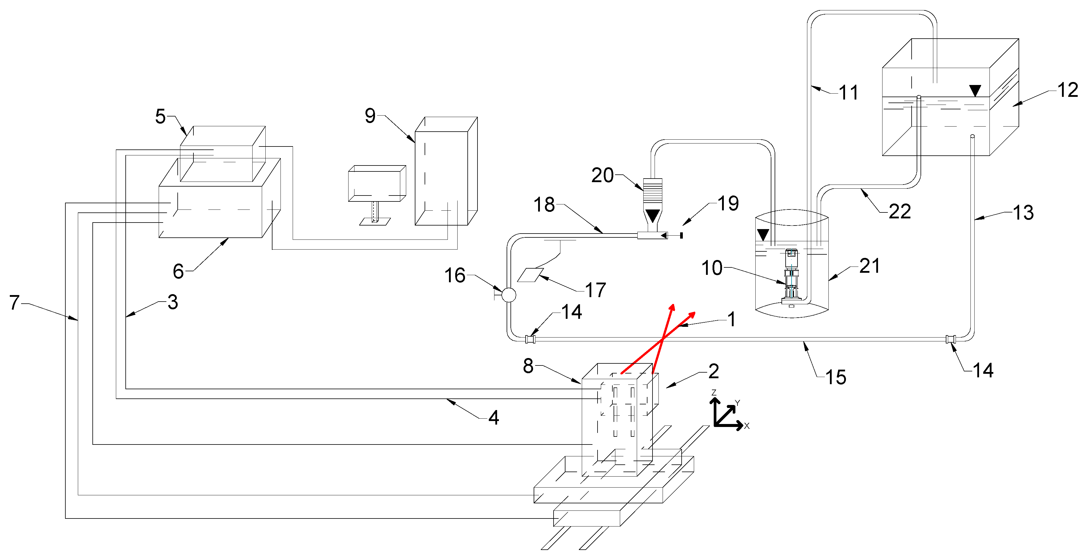
Figure 1. The system of apparatus [15]: 1—laser beams, 2—LDA optical system, 3—optical fiber, 4—return signal wire, 5—laser Doppler anemometer, 6—traverse controller, 7—x,y,z movement signal wires, 8—system of the optical benches with engines, 9—microcomputer, 10—pump, 11—supply pipe, 12—upper tank, 13—inlet pipe, 14—straight coupler, 15—transparent tube, 16—valve, 17—thermometer, 18—outlet pipe, 19—adjustment valve, 20—float meter, 21—bottom tank, 22—overflow pipe.
Environsciproc 09 00012 g001
Figure 2. The plot of the regression line and experimental results.
Environsciproc 09 00012 g002
Publisher’s Note: MDPI stays neutral with regard to jurisdictional claims in published maps and institutional affiliations.