Article

Predicting the Compression Capacity of Screw Piles in Sand Using Machine Learning Trained on Finite Element Analysis

1
Department of Civil, Structural and Environmental Engineering, Trinity College Dublin, College Green, Dublin 2, D02 PN40 Dublin, Ireland
2
Department of Civil Engineering, Azarbaijan Shahid Madani University, Tabriz 5375171379, Iran
*
Author to whom correspondence should be addressed.
Geotechnics 2024, 4(3), 807-823; https://doi.org/10.3390/geotechnics4030042
Submission received: 10 July 2024 / Revised: 4 August 2024 / Accepted: 13 August 2024 / Published: 21 August 2024
(This article belongs to the Special Issue Recent Advances in Geotechnical Engineering (2nd Edition))

Abstract

:
Screw piles (often referred to as helical piles) are widely used to resist axial and lateral loads as deep foundations. Multi-helix piles experience complex interactions between the plates which depend on the soil properties, pile stiffness, helix diameter, and the number of helix plates among other factors. Design methods for these piles are typically highly empirical and there remains significant uncertainty around calculating the compression capacity. In this study, a database of 1667 3D finite element analyses was developed to better understand the effect of different inputs on the compression capacity of screw piles in clean sands. Following development of the numerical database, various machine learning methods such as linear regression, neural networks, support vector machines, and Gaussian process regression (GPR) models were trained and tested on the database in order to develop a prediction tool for the pile compression capacity. GPR models, trained on the numerical data, provided excellent predictions of the screw pile compression capacity. The test dataset root mean square error (RMSE) of 29 kN from the GPR model was almost an order of magnitude better than the RMSE of 225 kN from a traditional theoretical approach, highlighting the potential of machine learning methods for predicting the compression capacity of screw piles in homogenous sands.

1. Introduction

The use of screw piles has increased significantly in recent years mainly due to their excellent performance under axial loading, their relatively low noise and vibration compared to impact driven piles, and their suitability for a wide range of ground conditions. The in-service performance of the screw piles largely depends on the embedded pile length L, helix diameter D, pile shaft diameter d, spacing between the helix plates S (for multi-helix anchors), installation method, as well as the properties of the soil deposit. Screw piles are ideally installed in a pitch-matched manner [1] to avoid disturbance to the soil which could then have a detrimental effect on post-installation pile capacity [2]. Pitch-matching is where the rate of vertical advancement of the pile per rotation Δ z , corresponds to the distance between the helix leading edge and the end of the helix and is usually defined with the advancement ratio AR:
A R = Δ z P h
where P h is the geometric pitch of the helical plate. Sharif et al. [2] suggested that the torque required to install a screw pile can be predicted based upon a unique factor that relates the observed installation torque to pile capacity, which is typically determined based upon published empirical techniques (for example [1]). Therefore, predicting the screw piles capacity can be important for assessing both installation and in-service performance. Current methods for predicting the compression capacity of screw piles rely on empirical factors to account for the efficiency of load transfer between helix plates. These empirical factors tend to follow simple linear equations and are dependent on a small number of variables (e.g., soil friction angle, and normalized spacing). These simple factors are incapable of fully capturing the complex interaction behavior between the screw pile helix plates.
Several studies have investigated the effect of inter-helix spacing on the load transfer mechanism of screw piles in sands. For multi-helix piles, two modes of failure have been suggested: (1) cylindrical shear (CS, also referred to as perimeter shear or envelope failure) between adjacent plates and (2) individual plate bearing [3]. Livneh and El Naggar [4] investigated the behavior of the screw piles under axial compressive and tensile loads through full-scale testing and numerical modelling. They suggested that the ground-line load–displacement response of a screw pile consisted of three distinct stages: (I) a linear elastic stage, (II) a nonlinear stage with little interaction between helix plates (individual plate bearing), and (III) a near-linear stage where significant interaction occurs between the helix plates and a cylindrical shear failure mechanism forms around the trailing helix plates. Alwan and El Naggar [5] used 3D finite element (FE) modelling to study the load transfer mechanism of screw piles with various normalized helix spacing (S/D) and showed that the load transfer mechanism of the screw piles depends on the selected failure criteria. They demonstrated that the load-transfer mechanism in compression is primarily cylindrical shear for S/D = 1 and individual plate bearing for S/D ≥ 1.5 based on a failure criteria of 25 mm (≈5% of D) displacement at pile head. Using a failure criteria of 8–10% of D at pile head, the cylindrical shear behavior was dominant for spacing ratio ≤ 1.5, and individual plate bearing governed for S/D > 1.5. They further suggested that using a failure criteria of 12% of D, the load transfer is cylindrical shear for S/D ≤ 2, and individual plate bearing for S/D ≥ 3. Zhang [6] suggested that for screw piles in sand with S/D < 2, cylindrical shear behavior will occur. Donal and Calyton [7] and Livro [8] reported when S/D > 3 independent plate bearing will occur. Moreover, Salhi et al. [9] reported for S/D = 1.5–2 is the optimal normalized helix spacing, and Knappet et al. [10] recommended an S/D > 3 for individual plate bearing in sandy soil.
Elsherbiny and El Naggar [11] studied the axial response of the helical piles through numerical analyses and field tests. They proposed a method for calculating the bearing capacity of double helix screw piles in sand which included a reduction factor and helix efficiency factor to account for interaction between the helix plates. They suggested the theoretical compressive capacity, Q c , of a screw pile at a normalized displacement of 5% of diameter can be given by the following:
Q c = γ H 2 A 2 N q R + E h γ H 1 A 1 N q R + π d 2 H e f f 2 γ K s tan δ
where:
γ is the effective unit weight of the soil
H 2 is the depth to bottom helix
A 2 is the surface area of bottom helix
N q is the bearing capacity factor (= e π tan ϕ tan 2 45 + ϕ 2 )
D is the helix diameter
d is the shaft diameter
H 1 is the depth to top helix
A 1 is the surface area of top helix
ϕ is the soil peak angle of internal friction
δ is the shaft–soil interface friction angle (=0.65 ϕ adopted in this paper)
H e f f is the effective shaft length (= H 1 D )
R is a bearing capacity reduction factor
E h is a helix efficiency factor
There is little agreement in the literature for the optimum value of the normalized helix spacing. Many of the previous experimental studies focused on the response from full-scale tests where it was not possible to identify the development of soil strains between helix plates during loading. The complex soil-structure interaction with multiple dependent soil and geometric parameters makes it challenging for traditional theoretical methods to fully capture the response.
Machine learning (ML) methods offer a more powerful means of capturing this complex behavior compared with traditional theoretical approaches. Machine learning methods have been applied to numerous problems in geotechnical analysis including for estimating the capacity of driven piles ([12,13,14] and others), bored piles ([15,16], and others). For screw piles, Wang et al. [17] employed artificial neural networks (ANN) to predict the uplift capacity of screw piles in sand, based on data from 36 small-scale laboratory tests. Similarly, Wang et al. [18] used gradient-boosting decision trees, fine-tuned with particle swarm optimization on a dataset derived from centrifuge tests. Peres et al. [19] employed ML techniques to predict the installation torque of helical piles. Nevertheless, the literature on the application of machine learning (ML) in the design of helical piles remains limited.
In this study, the relationship between the pile response and the load bearing mechanism of the screw piles with different spacing of helix plates under compressive loading in sands was investigated through 3D finite element (FE) modelling. Screw piles with different inter-helix spacing, length, and helix diameter with varying soil properties were modelled in 3DFE and analyzed under compressive loading. A number of different ML models were then trained on the outputs of the 3DFE models to provide a tool capable of predicting the pile capacity with improved accuracy over the traditional theoretical methods with minimum computation time. Further insights into the effect of inter-helix spacing and other parameters were obtained through the trained ML models.

2. 3D FE Modelling

2.1. Methodology

An FE model was developed using the Plaxis 3D (v20) software to simulate the screw pile behavior. An extensive parametric study to further the understanding of the behavior of helical piles in different soil conditions was undertaken. In all analysis cases the soil was modelled using the linear elastic-perfectly plastic Mohr–Coulomb constitutive soil model in Plaxis. The helix plates were simplified as circular disks without pitch, and a linear elastic model was used to represent the pile materials, as specified in Table 1. The width and breadth of all models was 40 × 40 m and the depth of the model was 30 m in order to minimize boundary effects on the results of numerical analyses (see Figure 1b). Mesh generation was undertaken with fine 15-node triangular elements and a very fine local meshing was applied in the vicinity of the pile because of considerable changes of soil stresses and strains in this zone. The pile shaft and helix plates were modelled by plate elements with virtual thickness. To simulate the pile and soil interaction, interface elements with property based on Mohr–Coulomb criteria with shear strength reduction factor of (Rint) 0.65 were selected [20]. The piles were wished-in-place and no installation effects were considered (discussed later). The authors acknowledge that 2D axis-symmetric FE analysis would offer similar accuracy and significant improvements in computation time, however, this was unavailable to the authors at the time of undertaking the analysis.

2.2. Validation

In order to validate the 3DFE modelling approach, three separate field test piles from the literature were modelled and the groundline response was compared with the field test results. Sakr [21] performed full-scale tests to investigate the axial capacity of screw piles in sand. The ST-1 test reported in [21] had an embedded length, L, of 9 m and shaft diameter, d, of 0.324 m, and a helix diameter, D, of 0.76 m, installed in medium to dense sand, was selected to calibrate the numerical analyses. The soil properties used were adopted directly from Sakr [21] and are provided in Table 2. Elsherbiny and El Naggar [11] performed 5 screw pile tests in sand with pile PA-1 being selected for validations in this paper. Pile PA-1 is a single helix pile with an embedded length, L, of 5.5 m and helix diameter, D, of 0.61 m, embedded in a medium-dense sand deposit. The soil properties adopted in modelling PA-1 are given in Table 3. Livneh and El Naggar [4] carried out field tests at two clayey silt sites (site 1 and site 2). While silt/clayey sites are not the focus of the paper, this validation is included to further showcase the performance of the FE modelling approach. The test performed at site 1 with properties listed in Table 4 were considered for validation in this study. Figure 2 shows that in all three cases, the 3DFE provided excellent predictions of the field test response.

2.3. Developing 3DFE Dataset

In order to investigate the effect of helix spacing on the screw pile response, two batches of analyses with a total 1667 3DFE models were conducted. In all models, dry sand was assumed with the water table supposed to be well below the base of the model. The results from these analyses were interrogated to examine the influence of different input parameters on the load–displacement response. For batch 1 analyses, the base case pile geometry and soil conditions were used and the helix spacing (S) was varied. The patterns of shear strain development around screw piles with different helix spacing was studied. In batch 2 analyses, the soil conditions and pile geometries were varied to provide a database with more general applicability. The base case pile geometry used in batch 1 analyses considers a 3-helix pile with length (L) of 10 m, shaft diameter (d) of 0.1 m, helix diameter (D) of 0.4 m and helix thickness of 0.02 m. The base case soil considered in this study was a medium dense sand, with specification listed in Table 5.
For batch 2 analyses, the screw pile geometry and soil properties were varied (7 different input features) using different combinations of the values shown in Table 6. Each 3DFE model used a homogenous soil profile or pile geometry. The values in Table 6 were chosen to cover the range of values of screw pile experiments reported in the literature.

3. FE Modelling Results

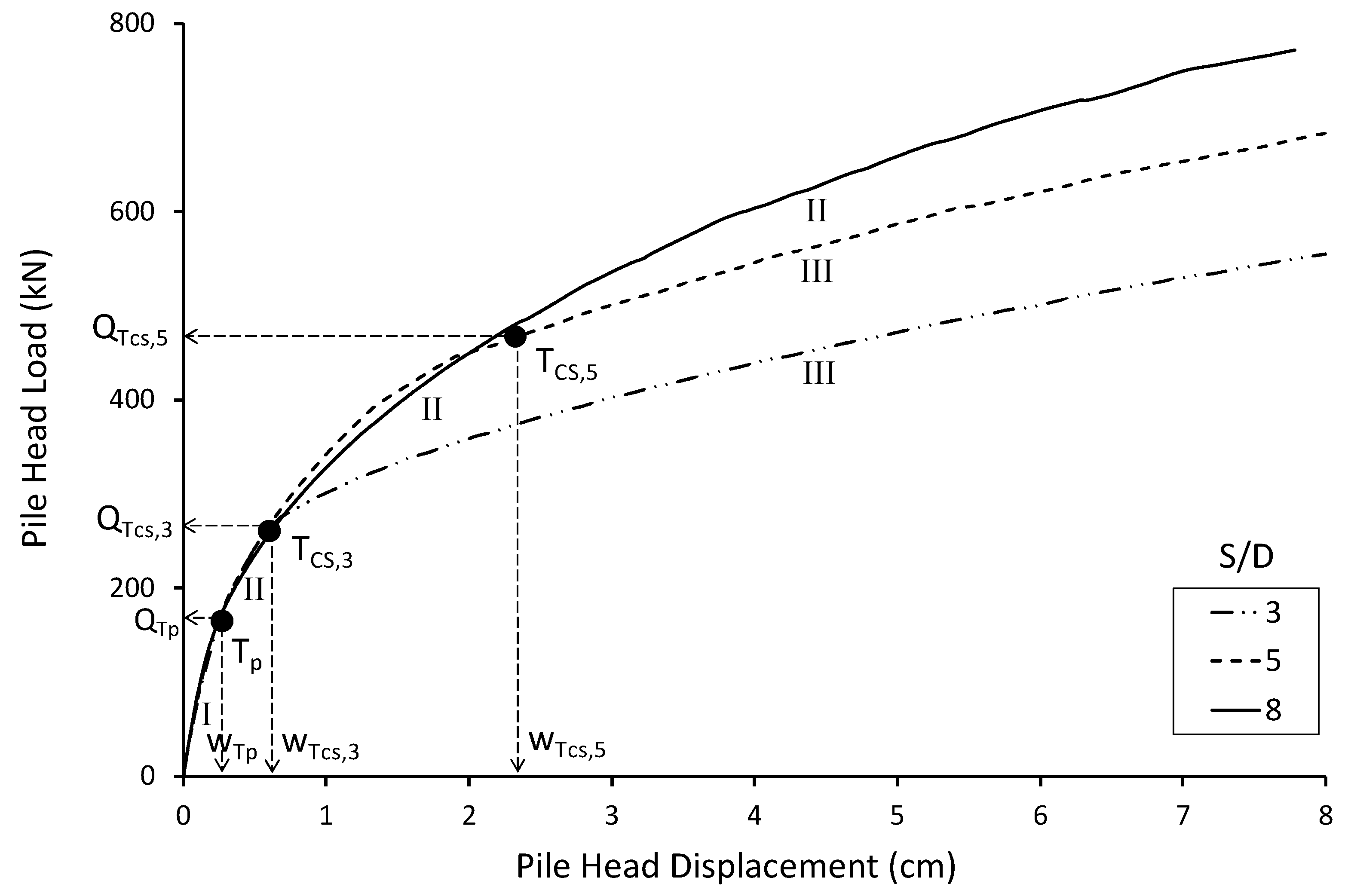
Figure 3 shows that the axial load–displacement response for screw piles in compression can be considered as three stages as described by Livneh and El Naggar [4]. The pile load–displacement response as well as the development of shear strain within the soil around screw piles with inter-helix spacing of small (S/D = 3), moderate (S/D = 5), and large (S/D = 8) are presented in Figure 4, Figure 5 and Figure 6. For S/D > 6 little interaction occurs between the plates and therefore the curve is restricted to the stages I and II (i.e., stage III is never reached). The displacement at which the transition between elastic stages I and plastic stage II occurs is referred to as the plastic transition point (wTp) and the displacement at which the transition between II (no helix interaction) and III (helix interaction) occurs is referred to as cylindrical shear transition point wTcs (see Figure 3). The plastic transition point wTp appears to be independent of the inter-helix spacing while the distance between wTp and wTcs increases with the values of S/D as would be expected (as larger displacement is required to mobilize interaction between the plates which are further apart). The loads corresponding to displacements wTp and wTcs are referred to as the plastic transition load QTp and the cylindrical shear transition load, QTcs.
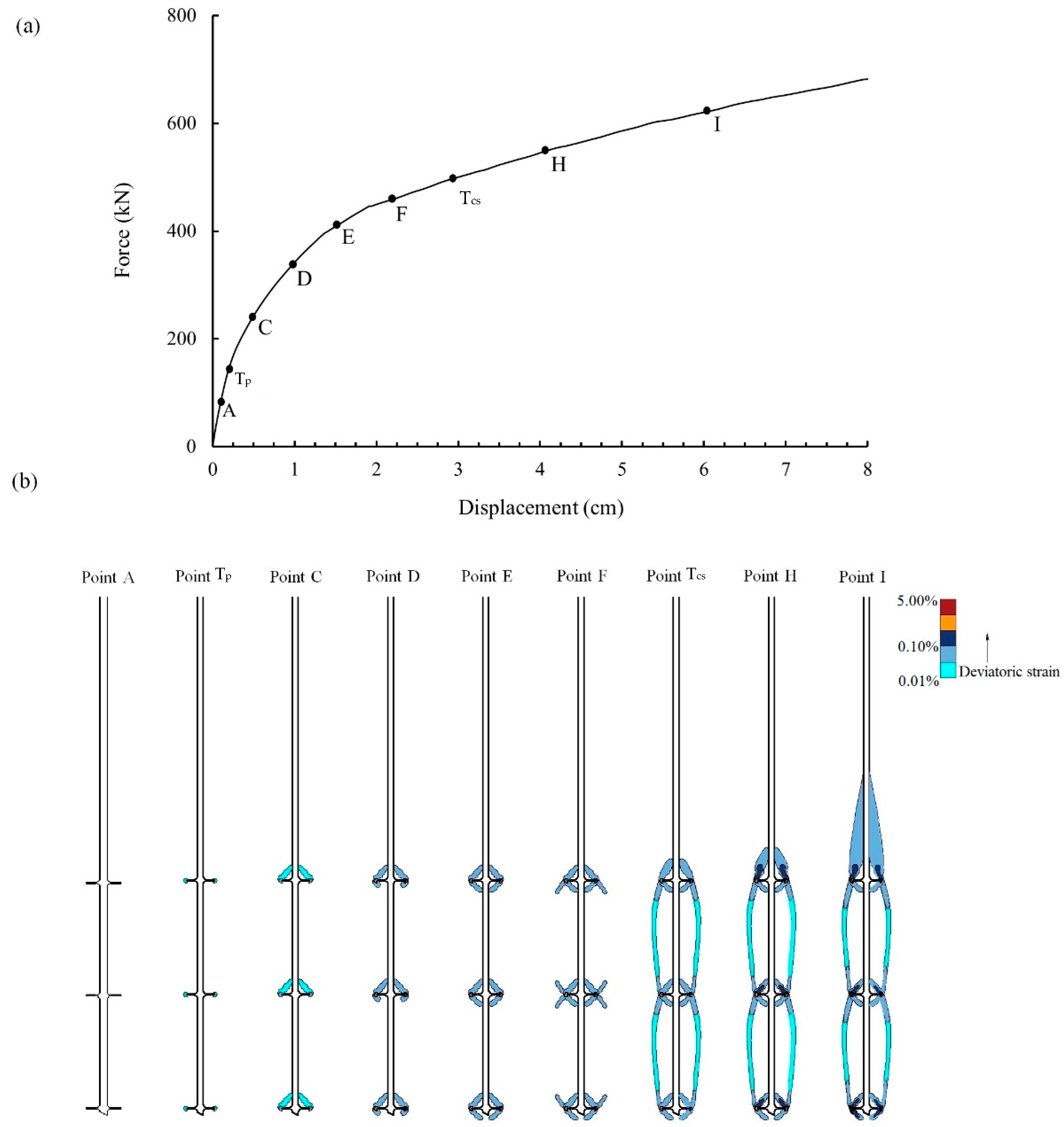
For piles with small S/D < 3, shown in Figure 4, the shear strains initially form at the vicinity of helix plates, when the loading value passes QTp and the soil response moves from elastic (stage I) to plastic (stage II). As the loading increases, the shear strains around each helix plate develop and create a cylindrical shear zone when the force reaches QTcs and the pile response enters stage III. As the loading increases further, the magnitudes of the shear strains between the helix plates increase and the strained zone spreads toward the ground surface from the top plate (see points D to F in Figure 4b). These patterns are in agreement with those reported by [6,9,10,22]. For piles with an S/D of 5 (shown in Figure 5), similar behavior was noted. As the load increases from QTp, the shear strains were first concentrated in the vicinity of the helix plates (stage II) and eventually extended within the soil between the helix plates to form the cylindrical shear zone when the applied load exceeded QTcs (stage III). In this case, much larger displacements, wtcs, were required to mobilize the cylindrical shear zone. For piles with an S/D of 8 (shown in Figure 6), the first two stages were noted. It is clear from Figure 6b that full plate interaction and the cylindrical shear zone do not form even after large displacements.

4. Application of Machine Learning Methods to Predict Compression Capacity

4.1. Training and Testing Datasets

In order to develop datasets for training and testing machine learning models, the full dataset of 1667 3DFE models was postprocessed to extract the compression capacity (Qc), which in this paper was defined as a load that produces a vertical settlement of 10 percent of the largest helix diameter [23]. The dataset used seven input features including pile geometrical input features pile diameter D, normalized helix spacing S/D, number of helix plates n, and pile embedded length L, along with soil features of peak friction angle ϕ , soil Young’s modulus E, and soil unit weight. The target feature was the compression capacity (Qc). The compression capacity from each 3DFE model along with the input features form the training and testing samples (one sample per 3DFE model). For the training and validation 80% of the 1667 samples were randomly selected while the remaining 20% were retained as the holdout (or test) dataset for testing the trained models. To compare the performance of different ML models 10-fold cross validation was used on the training dataset and these validation metrics were compared along with the test dataset metrics to assess the best performing models.

4.2. Machine Learning Models

In this paper, 27 different machine learning models were trained using the regression learner application in Matlab [24] to quickly assess which machine learning models performed best. The application provides tools for model training, including cross-validation, to prevent overfitting and ensure generalizability. Performance metrics such as root mean squared error (RMSE), mean absolute error (MAE), and coefficient of determination (R-squared) were used for model evaluation. The machine learning methods tested include the following:
  • Linear regression models: Simple and multiple linear regression, enabling the modelling of relationships between predictors and a continuous response variable.
  • Support vector machines (SVM) with various kernel functions (linear, quadratic, cubic, and Gaussian).
  • Decision trees and ensembles: Including regression trees, bagged trees, boosted trees, and random forests.
  • Gaussian process regression (GPR): With different kernel functions (squared exponential, Matern, rational quadratic, etc.).
  • Neural networks: Bilayer and trilayer basic feedforward neural networks which can model complex, non-linear relationships through hidden layers.
Further description of the mathematical basis for the various ML models can be found in Sheil et al. [25]. The default models as per the Matlab regression learner app [24] were used. All the GPR and NN models were trained using the hyperparameter settings as listed in Table 7 and Table 8, respectively. Each of the 27 models were trained on the training dataset. The models were then used to predict the compression capacity for the testing dataset.

5. Results and Discussion

The list of ML models trained and the performance metrics for each model are compared in Table 9. The table is ranked based on the RMSE of the test dataset. The best performing models were Gaussian process regression models followed by neural networks. The single best performing model, ranked based on RMSE test and MAE test, was the rational quadratic Gaussian process regression (RQGPR). Other GPR models with different kernel functions (e.g., Matern 5/2 GPR and squared exponential GPR) had similar performance metrics.
In order to further explore the model capability and to assess how much training data (i.e., 3DFE models) was needed to train the model with high accuracy, the RQGPR model was selected and retrained with subsets of the training dataset, starting with 2% of the full training dataset and increasing in increments of 2% up to 100%. The effect of the training set size on the RMSE for the RQGPR model is shown in Figure 7a. Substantial improvement in both test and validation performance is seen up to a training set size of ~200 samples, after which the rate of improvement decreases before levelling out at around 600 samples. Only marginal improvement in both validation and test RMSE is seen, once more than 600 samples are used.
For the RQGPR models trained on the full training dataset, the predicted response is plotted against the true response (from 3DFE models) in Figure 7b for both the training dataset (blue circles) and testing dataset (red circles). It can be seen, as reflected in the performance metrics, that that RQGPR provides excellent predictions for both the training and testing datasets. For comparison with traditional capacity calculation methods, the theoretical pile capacity prediction approach proposed by Elsherbiny and El Naggar [11], was implemented in Matlab and used to calculate the compression capacity (green cross). The RMSE for the theoretical approach is 225 kN, almost an order of magnitude greater than the RMSE of 29 kN from the RQGPR model. It is evident that the trained RQGPR significantly outperforms the theoretical approach in this case.
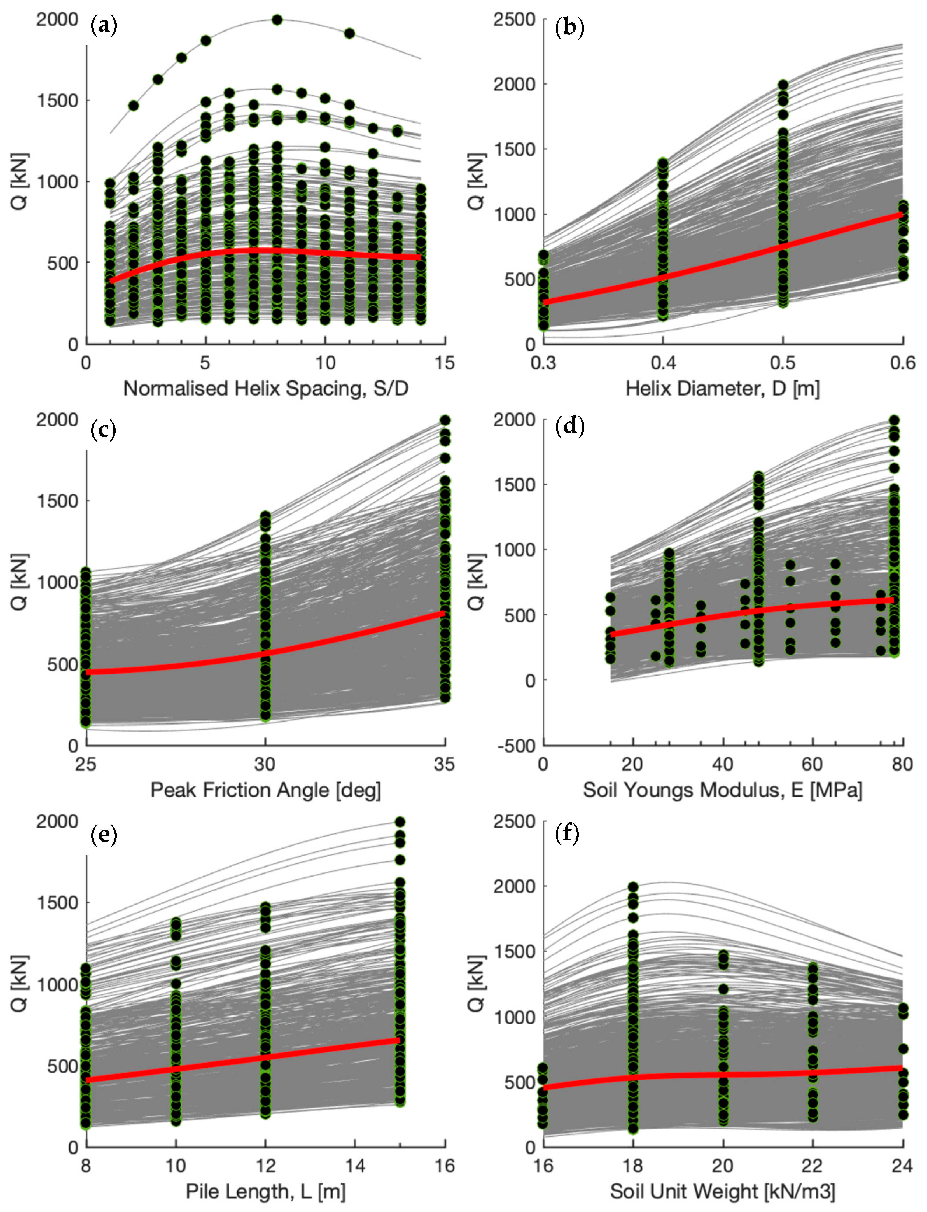
The GPR model can also be used to provide insights into the influence of different features on the pile capacity. Conditional expectation plots for each input feature are provided in Figure 8. On average, the effect of increasing normalized helix spacing, S/D, can be seen to significantly increase pile capacity up until a helix spacing of between 6 to 7 after which further increase of the spacing has no influence. Therefore, the optimum S/D ratio based on this analysis is considered to be approximately 6. The effect of increasing helix diameter D, pile length L, or soil unit weight γ are seen to have an almost linear increase in pile capacity. Increasing the friction angle is seen to have a non-linear convex response while increasing the soil Young’s modulus is seen to have a non-linear concave response.
There are a number of limitations in the analysis provided in this paper which require further discussion:
  • The linear elastic perfectly plastic constitutive soil model was used for the 3DFE analysis. This model is the most widely used constitutive model for soil behavior, but it has limitations compared to more advanced models. Its advantages include its straightforward formulation, making it easy to understand simple input parameters which are intuitive and easy to obtain from common soil tests, and it is computationally efficient compared to more complex models. However, it should be noted that significant drawbacks include its inability to accurately capture the soil strength as described by critical state soil mechanics, its inability to capture nonlinear stress–strain behavior, and its inability to account for the evolution of soil fabric anisotropy under loading. Future work will focus on the use of more advanced soil models, such as the SANISAND family of models, to provide more accurate predictions of the soil response. It should also be noted that the 3DFE analysis used in this paper did not include installation effects, which have been shown to have a significant influence on the response of screw piles, particularly regarding the pullout resistance [2,26].
  • The database 3DFE model was initially developed in an adhoc manner and therefore not optimized to provide the best ML training outcomes with the minimum number of models. Potential biases exist within the dataset where sample points may be clustered around certain input features. Better planning at an early stage and using approaches such as Latin hypercube, Sobol sampling, or active learning approaches may require fewer FE models to achieve similar ML model accuracy. Future work will explore the use of different sampling strategies to optimize the production of training data and the training of the ML models.
  • All the 3DFE models analyzed in this paper assumed dry homogenous sand. Future work will explore the effect of water table depth and layered soils on the compression capacity [27].
  • Future work will also focus on using physics informed machine learning approaches and incorporating multi-modal data, for example low-fidelity theoretical models along with high-fidelity 3DFE models and experimental field test data, similar to the approach suggested in Surysentana et al. [28].

6. Conclusions

In this study a database of 1667 3DFE models was created in order to explore the factors which affect the bearing capacity of screw piles in dry sand. Machine learning models including linear regression, neural networks, support vector machines and Gaussian process regression models were then trained on the numerical database in order to develop a predictive tool for quickly estimating the screw pile capacity. The main conclusions were the following:
  • Out of the 27 different machine learning models tested, Gaussian process regression models offered the best performance when ranked based on MAE on the test dataset. The ML models offered an almost 10-fold improvement in RMSE when compared with traditional theoretical methods.
  • The best performing model ranked based on MAE (test) and RMSE (test) was the rational quadratic Gaussian process regression (RQGPR). This model was explored further. Training the model using subsets of the full training database indicated very good predictions could be obtained using only 200 randomly selected training samples (3DFE models), and only marginal improvements were seen once the number of training samples increased beyond 600. Similar accuracy could potentially be achieved with less training data through improved parameter space sampling methods such as Latin hypercube sampling or the Sobol methods.
  • Further insights into the factors affecting the screw pile capacity were obtained through conditional expectation plots which indicate an inter-helix spacing of ~6 helix diameters may be optimum.
  • Traditional theoretical methods used for screw pile design suffer from an inability to fully capture the complex soil-structure interaction which occurs in multi-helix screw piles. This paper shows the potential for ML models as a design tool which can have significantly higher accuracy than traditional design approaches. Future work will focus on training ML models on multi-modal data including field test results.
  • The database developed in this paper and used for training and trained ML models has been made available open access on Github (https://github.com/igoed1/Screw-pile-3DFE-and-ML-models.git).

Author Contributions

Conceptualization, D.I. and P.Z.; 3DFE analysis, P.Z. and H.S.-J.; Machine learning analysis, D.I.; writing—original draft preparation, D.I. and P.Z.; writing—review and editing, D.I.; visualization, D.I. and P.Z.; supervision of 3DFE analysis, H.S.-J.; funding acquisition, D.I. All authors have read and agreed to the published version of the manuscript.

Funding

The authors are grateful for the financial support provided by the Science Foundation Ireland Centre for Applied Geosciences (ICRAG), grant number 13/RC/2092_2 who provided support for this work.

Data Availability Statement

The ML Dataset and Trained RQGPR model are available open access on Github (https://github.com/igoed1/Screw-pile-3DFE-and-ML-models.git).

Conflicts of Interest

The authors declare no conflicts of interest. The funders had no role in the design of the study; in the collection, analyses, or interpretation of data; in the writing of the manuscript; or in the decision to publish the results.

References

  1. Perko, H.A. Helical Piles: A Practical Guide to Design and Installation; John Wiley & Sons, Inc.: Denver, CO, USA, 2009. [Google Scholar] [CrossRef]
  2. Sharif, Y.U.; Brown, M.J.; Cerfontaine, B.; Davidson, C.; Ciantia, M.; Knappett, J.; Brennan, A.; Ball, J.D.; Augarde, C.; Coombs, W.; et al. Effects of screw pile installation on installation requirements and in-service performance using the Discrete Element Method. Can. Geotech. J. 2021, 58, 1334–1350. [Google Scholar] [CrossRef]
  3. Lutenegger, A.J. Screw piles and helical anchors—What we know and what we don’t know: An academic perspective. In Proceedings of the International Symposium on Screw Piles for Energy Applications, West Park Dundee, UK, 27–28 May 2019. [Google Scholar]
  4. Livneh, B.; El Naggar, M.H. Axial testing and numerical modeling of square shaft helical piles under compressive and tensile loading. Can. Geotech. J. 2008, 45, 1142–1155. [Google Scholar]
  5. Alwalan, M.F.; El Naggar, M.H. Load-transfer mechanism of helical piles under compressive and impact loading. Int. J. Geomech. 2021, 21, 04021082. [Google Scholar]
  6. Zhang, D. Predicting Capacity of Helical Screw Piles in Alberta Soils. MSc. Thesis, University of Alberta, Edmonton, AB, Canada, 1999. [Google Scholar]
  7. Donal, J.; Calyton, P.E. Basic Helical Screw Pile Design. ECP Torque Anchor Brand of Helical Screw Piles; Earth Contact Products: Olathe, Kansas, 2005; pp. 1–28. [Google Scholar]
  8. Livro. Helical Pile Engineering Handbook, 7th ed.; Helical Pier Systems: Nisku, AB, Canada, 2010; pp. 20–28. Available online: www.helicalpiersystems.com (accessed on 9 July 2024).
  9. Salhi, L.; Nait-Rabah, O.; Deyrat, C.; Roos, C. Numerical modeling of single helical pile behavior under compressive loading in sand. Electron. J. Geotech. Eng. 2013, 18, 4319–4338. [Google Scholar]
  10. Knappet, J.A.; Brown, M.J.; Brennan, A.J.; Hamilton, L. Optimising the compressive behaviour of screw piles in sand for marine renewable energy applications. In Proceedings of the DFI/EFFC 11th International Conference on Piling and Deep Foundations, Stockholm Fair, Stockholm, Sweden, 21–23 May 2014. [Google Scholar]
  11. Elsherbiny, Z.H.; El Naggar, M.H. Axial compressive capacity of helical piles from field tests and numerical study. Can. Geotech. J. 2013, 50, 1191–1203. [Google Scholar]
  12. Samui, P. Prediction of friction capacity of driven piles in clay using the support vector machine. Can. Geotech. J. 2008, 45, 288–295. [Google Scholar]
  13. Liu, Y.; Liang, S.; Wu, J.; Fu, N. Prediction method of vertical ultimate bearing capacity of single pile based on support vector machine. Adv. Mater. Res. 2011, 168–170, 2278–2282. [Google Scholar]
  14. Zhang, M.; Liang, L.; Song, H.; Li, Y.; Peng, W. Intelligent prediction for side friction of large-diameter and super-long steel pipe pile based on support vector machine. Appl. Mech. Mater. 2012, 170–173, 747–750. [Google Scholar]
  15. Kordjazi, A.; Pooya Nejad, F.; Jaksa, M.B. Prediction of ultimate axial load-carrying capacity of piles using a support vector machine based on CPT data. Comput. Geotech. 2014, 55, 91–102. [Google Scholar] [CrossRef]
  16. Kardani, N.; Zhou, A.; Nazem, M.; Shen, S.L. Estimation of Bearing Capacity of Piles in Cohesionless Soil Using Optimised Machine Learning Approaches. Geotech. Geol. Eng. 2020, 38, 2271–2291. [Google Scholar] [CrossRef]
  17. Wang, B.; Moayedi, H.; Nguyen, H.; Foong, L.K.; Rashid, A.S.A. Feasibility of a novel predictive technique based on artificial neural network optimized with particle swarm optimization estimating pullout bearing capacity of helical piles. Eng. Comput. 2020, 36, 1315–1324. [Google Scholar]
  18. Wang, L.; Wu, M.; Chen, H.; Hao, D.; Tian, Y.; Qi, C. Efficient Machine Learning Models for the Uplift Behavior of Helical Anchors in Dense Sand for Wind Energy Harvesting. Appl. Sci. 2022, 12, 10397. [Google Scholar] [CrossRef]
  19. Peres, M.S.; Schiavon, J.A.; Ribeiro, D.B. A Machine Learning-Based Approach for Predicting Installation Torque of Helical Piles from SPT Data. Buildings 2024, 14, 1326. [Google Scholar] [CrossRef]
  20. Brinkgrevee, R.B.J.; Broere, W.; Waterman, D. Plaxis V8, Reference Manual; Delft University of Technology and PLAXIS: Delft, The Netherlands, 2002. [Google Scholar]
  21. Sakr, M. Installation and performance characteristics of high capacity helical piles in cohesionless soils. DFI J. 2011, 5, 39–57. [Google Scholar]
  22. Mitsch, M.P.; Clemence, S.P. The uplift capacity of helix anchors in sand. In Proceedings of the Uplift Behavior of Anchor Foundations in Soil: A Session Sponsored by the Geotech; American Society of Civil Engineers: Reston, VA, USA, 1985. [Google Scholar]
  23. Mohajerani, A.; Bosnjak, D.; Bromwich, D. Analysis and design methods of screw piles: A review. Soils Found. 2016, 56, 115–128. [Google Scholar]
  24. Matlab. Available online: https://uk.mathworks.com/help/stats/regression-learner-app (accessed on 25 June 2024).
  25. Sheil, B.B.; Suryasentana, S.K.; Mooney, M.A.; Zhu, H. Machine learning to inform tunnelling operations: Recent advances and future trends. Proc. ICE–Smart Infrastruct. Constr. 2020, 173, 74–95. [Google Scholar] [CrossRef]
  26. Cerfontaine, B.; White, D.; Kwa, K.; Gourvenec, S.; Knappett, J.; Brown, M. Anchor geotechnics for floating offshore wind: Current technologies and future innovations. Ocean Eng. 2023, 279, 114327. [Google Scholar] [CrossRef]
  27. Yan, G.; Li, Z.; Galindo Torres, S.A.; Scheuermann, A.; Li, L. Transient Two-Phase Flow in Porous Media: A Literature Review and Engineering Application in Geotechnics. Geotechnics 2022, 2, 32–90. [Google Scholar] [CrossRef]
  28. Suryentana, S.; Sheil, B.; Stuyts, B. Practical Approach for Data-Efficient Metamodeling and Real-Time Modeling of Monopiles Using Physics-Informed Multifidelity Data Fusion. J. Geotech. Geoenviron. Eng. 2024, 150, 06024005. [Google Scholar] [CrossRef]
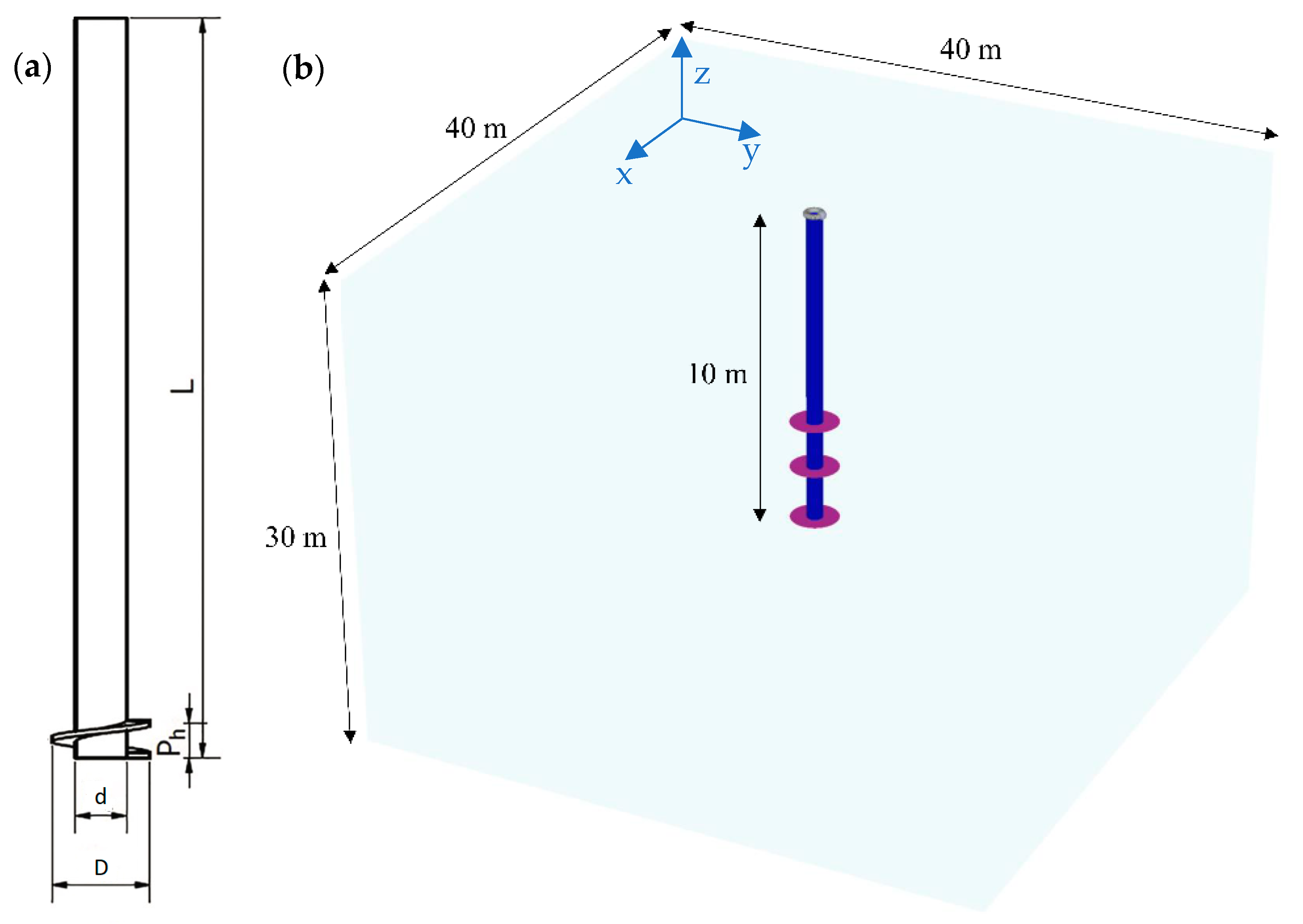
Figure 1. (a) Screw pile geometry (adapted from [2]) and (b) dimensions of the 3DFE model.
Geotechnics 04 00042 g001
Figure 2. Validation of 3DFE modelling against field test data from (a) Sakr [21], (b) Livneh and El Naggar [11] and (c) Elsherbiny and El Naggar [4].
Geotechnics 04 00042 g002
Figure 3. The schematic presentation of axial load–displacement response of a screw pile with different S/D values showing the transition point from elastic to plastic behavior (Tp) and transition point from individual plate bearing to cylindrical shear behavior (Tcs) with corresponding load (Q) and displacement (w).
Geotechnics 04 00042 g003
Figure 4. Batch 1 analysis (a) ground-line load–displacement response of screw pile with inter-helix spacing ratio (S/D) of 3, (b) distribution of shear strains around helix plates at given ground-line displacements.
Geotechnics 04 00042 g004
Figure 5. Batch 1 analysis (a) ground-line load–displacement response of screw pile with inter-helix spacing ratio (S/D) of 5, (b) distribution of shear strains around helix plates at given ground-line displacements.
Geotechnics 04 00042 g005
Figure 6. Batch 1 analysis (a) ground-line load–displacement response of screw pile with inter-helix spacing ratio (S/D) of 8, (b) distribution of shear strains around helix plates at given ground-line displacements.
Geotechnics 04 00042 g006
Figure 7. (a) RMSE vs. training set size for RQGPR model and (b) predicted capacity vs. true capacity comparison between RQGPR model and theoretical pile capacity approach.
Geotechnics 04 00042 g007
Figure 8. Batch 2 analysis partial dependence plot (red line) and individual conditional expectation (grey lines) for different input features: (a) Normalized Helix Spacing (S/D); (b) Helix Diameter (D); (c) Peak Friction Angle; (d) Soil Young’s Modulus; (e) Pile Embedded Length (L); and (f) Soil Unit Weight.
Geotechnics 04 00042 g008
Table 1. Pile material properties adopted in this paper.
ParametersValues
Poisson ratio, υ0.33
Pile unit weight, γ (kN/m3)78
Modulus of elasticity of pile, Ep (GPa)210
Table 2. Soil properties for ST-1 analysis (from [21]).
ParametersValues
Internal friction angle, ϕ (deg) 35
Dilation angle, ψ (deg)0
Cohesion, c (kPa)0.1
Poisson ratio, υ0.3
Unit weight, γ (kPa)18
Modulus of elasticity, E (MPa)50
Table 3. Soil properties for PA-1 analysis (from [11]).
ParametersValues
Internal friction angle, ϕ (deg) 25
Dilation angle, ψ (deg)0
Cohesion, c (kPa)0.1
Poisson ratio, υ0.3
Unit weight, γ (kPa)20
Modulus of elasticity, E (MPa)50
Table 4. Soil properties for site 1 analysis (from [4]).
LayersDepth to (m)γ
(kN/m3)
c
(kPa)
ϕ
(deg)
E
(MPa)
Stiff brown sandy clayey silt2.417.31028100
Very stiff brown clayey silt4.117.5212785
Stiff grey clayey silt5.816.5923100
Very stiff grey sandy clayey silt7.3152030400
Dense grey silt>7.317193465
Table 5. Base case soil properties used for batch 1 analyses.
Soil Input ParametersValues
Internal friction angle, ϕ (deg) 30
Dilation angle, ψ (deg)0
Cohesion, c (kPa)0
Poisson ratio, υ0.33
Unit weight, γ (kPa)18
Modulus of elasticity, E (MPa)48
Table 6. The soil and pile geometrical features used in batch 2 analyses.
Feature NumberFeatureValue
1Unit weight, γ (kN/m3)16, 18, 20, 22
2Internal friction angle, ϕ (deg) 25, 30, 35
3Modulus of elasticity, E (MPa)18, 48, 78
4Number of helix plates, n2, 3
5Pile length, L (m)8, 10, 12, 15
6Helix diameter, D (m)0.3, 0.4, 0.5
7Inter–helix spacing ratio, S/D1–14
Table 7. Hyperparameter settings used in Gaussian process regression (GPR) models.
HyperparameterSetting
Basis Function Constant
Use Isotropic Kernel Yes
Kernel ScaleAutomatic
Signal Standard DeviationAutomatic
SigmaAutomatic
Standardize DataYes
Optimize Numeric ParametersYes
Table 8. Hyperparameter settings used in neural network (NN) models.
HyperparameterSetting
Number of Fully Connected LayersDefault = 1, Bilayered = 2, Trilayered = 3
Layer Size (all layers)Default = 10, Medium NN = 25, Wide NN = 100
ActivationReLu
Iteration Limit1000
Regularization Strength (Lambda)0
Standardize DataYes
Optimize Numeric ParametersYes
Table 9. Trained ML models and performance metrics.
Model TypeRMSE
(Validation)
R-Squared (Validation)MAE
(Validation)
MAE
(Test)
RMSE
(Test)
R-Squared
(Test)
Training Time
(s)
Rational Quadratic GPR33.10.9916.214.530.00.99130.0
Matern 5/2 GPR33.00.9916.114.630.30.9971.5
Squared Exponential GPR34.50.9918.116.330.90.9948.0
Trilayered Neural Network45.90.9725.523.135.80.98132.2
Medium Neural Network74.40.9341.022.336.10.9895.4
Exponential GPR38.60.9817.916.036.50.9874.5
Bilayered Neural Network56.00.9634.122.137.00.98116.9
Wide Neural Network43.50.9820.219.238.10.98114.4
Cubic SVM41.70.9822.921.538.70.9812.3
Medium Gaussian SVM43.10.9824.121.439.50.989.7
Least Squares Regression59.80.9639.633.954.40.96119.6
Quadratic SVM57.50.9635.136.260.30.969.1
Fine Tree77.20.9344.437.767.60.944.8
Narrow Neural Network71.20.9442.342.868.90.9491.4
Boosted Trees74.70.9347.144.373.90.9316.9
Bagged Trees76.50.9347.746.277.20.9318.4
Interactions Linear71.30.9447.650.377.70.937.2
Stepwise Linear71.80.9447.950.578.10.93117.6
Coarse Gaussian SVM89.60.9050.849.691.30.909.5
Medium Tree99.80.8866.564.5100.60.887.2
Linear109.80.8576.980.5117.60.838.4
Efficient Linear Least Squares111.50.8577.180.1118.00.8311.8
Fine Gaussian SVM124.90.8169.861.6119.70.838.6
Linear SVM116.60.8371.173.7122.80.827.7
Robust Linear127.20.8072.673.2131.20.795.8
Coarse Tree136.60.894.893.9140.30.86.7
SVM Kernel243.40.3163.5134.4224.10.4119.8
Efficient Linear SVM234.40.3173.7170.9230.60.411.5
Disclaimer/Publisher’s Note: The statements, opinions and data contained in all publications are solely those of the individual author(s) and contributor(s) and not of MDPI and/or the editor(s). MDPI and/or the editor(s) disclaim responsibility for any injury to people or property resulting from any ideas, methods, instructions or products referred to in the content.