Abstract
Three-dimensional transfer functions (3D TFs) are generally assumed to fully describe the transfer behavior of optical topography measuring instruments such as coherence scanning interferometers in the spatial frequency domain. Therefore, 3D TFs are supposed to be independent of the surface under investigation resulting in a clear separation of surface properties and transfer characteristics. In this paper, we show that the 3D TF of an interference microscope differs depending on whether the object is specularly reflecting or consists of point scatterers. In addition to the 3D TF of a point scatterer, we will derive an analytical expression for the 3D TF corresponding to specular surfaces and demonstrate this as being most relevant in practical applications of coherence scanning interferometry (CSI). We additionally study the effects of temporal coherence and disclose that in conventional CSI temporal coherence effects dominate. However, narrowband light sources are advantageous if high spatial frequency components of weak phase objects are to be resolved, whereas, for low-frequency phase objects of higher amplitude, the temporal coherence is less affecting. Finally, we present an approach that explains the different transfer characteristics of coherence peak and phase detection in CSI signal analysis.
1. Introduction
CSI is a well-established and widely used technique for many years. CSI instruments typically comprise Mirau, Michelson, and Linnik interference microscopes [1] (Chapter 15). Recently, progress has been made with respect to a full understanding of the transfer characteristics of these instruments [2,3,4,5,6,7,8,9,10]. An appropriate theoretical description of the transfer characteristics of CSI instruments is based on the physical optics or Kirchhoff approximation and results in a three-dimensional transfer function (3D TF), which represents not only the transfer range in the 3D spatial frequency domain but also the weighting of certain spatial frequency components [11,12,13,14,15,16,17]. The 3D TF is generally assumed to be independent of the surface under investigation. The surface can be mathematically treated by the foil model represented by a set of Dirac functions at certain height values depending on the -coordinates in the object space [3,15,17]. The 3D Fourier transform (3D FT) of this foil representation multiplied by the 3D TF results in the 3D Fourier transform of the image stack as it is obtained by a CSI measurement. Alternatively, the surface can be treated as a phase object [5,6,10,18]. According to Fourier optics, the 2D Fourier transform of the phase object with respect to the transverse coordinates x and y equals the 3D FT according to the foil model and thus can be multiplied by the 3D TF in order to obtain the 3D image stack by an inverse 3D FT [6,9].
This contribution is our third paper of a trilogy of current publications. First, we discussed the implications of the 3D TF bandwidth limitations in the context of CSI applications [6]. To achieve consistency, we introduced the double foil model that treats the reference wave field in the same way as the object field. However, the 3D TF used throughout this first paper was just an approximation. In our second contribution, we present a mostly analytical formula that enables the computation of the 3D TF of a microscope of high numerical aperture in reflection mode assuming monochromatic uniform spatially incoherent pupil illumination and a surface, which consists of point scatterers [19]. From the 3D TF obtained under this assumption, the familiar modulation transfer function (MTF) of a conventional microscope [20] results via integration along the axial spatial frequency coordinate. Furthermore, the 3D FT of this 3D TF results in a 3D point spread function (PSF) of a CSI system that perfectly fits to the point spread function obtained by an integration approach under the same assumptions [8].
However, to the best of our knowledge, all common approaches to 3D transfer functions of CSI instruments are valid under the assumption that the surface under investigation is characterized by single point scatterers. This consideration holds for rough surfaces, but CSI is often applied to measure objects with specularly reflecting surfaces or at least specularly reflecting surface structures. For confocal microscopes, it is well known that the transfer characteristics depend on whether the object under investigation is a point scatterer or a specular surface [21] (Chapter 1), [22] (Chapter 3).
In this contribution, we will show that also in CSI the 3D TF for a specularly reflecting surface differs from the 3D TF obtained in [19] for a scattering surface. We derive an analytical formula, which allows for quantifying these differences. Unfortunately, this complicates the modeling of CSI instruments, since, in some cases, the surface under investigation consists of both specular surface sections and sharp edges, at which a portion of the incident light is scattered. Note that specular surfaces encompass tilted plane mirrors as well as curved deterministic structures such as sinusoidal or chirped surfaces [23].
In order to motivate our study, we start with a phase object, i.e., the optical field on a surface immediately after reflection is given by
where represents the surface height function and is the axial spatial frequency, which depends on the wave number and thus on the wavelength of light as well as on the angle of incidence , the incident plane wave includes with the optical axis, i.e., the z-axis. For simplicity, (1) assumes constant reflectivity of the surface and unit amplitude of the reflected field. Considering all possible angles of incidence, the mean value of the axial spatial frequency is related to the so-called equivalent wavenumber by
Note that the phase object according to (1) can be also derived from the foil representation of the surface
via Fourier transform
The expression on the right-hand side of (1) is the first order Taylor series expansion and thus holds only for weak phase objects, where If the surface is a reflective one-dimensional sinusoidal diffraction grating of amplitude and period , which is translationally invariant with respect to the y coordinate, then
and the corresponding phase object can be expressed by the Fourier series
with the m-th order Bessel function of the first kind. Fourier transformation of the corresponding optical field with respect to the x and y coordinate results in:
where and are the transverse spatial frequencies. The last expression in (5) again holds for weak phase objects, i.e., for surface amplitudes, . If the surface amplitude is zero, i.e., ,
Due to the limited numerical aperture (NA) of the objective lens, the diffracted far-field is low-pass filtered with respect to the transverse spatial frequencies and bandpass filtered with respect to the axial spatial frequency. If the grating frequency is small enough to be transferred by the objective lens, the grating structure can be resolved. However, as soon as the low-pass filtering effect by the objective lens goes ahead with an attenuation of the first and higher order spatial frequency components compared to the zero order contribution represented by the first term in (5) the amplitude of the surface, reconstructed based on the measured phase values, will be attenuated too, i.e., the measured grating amplitude will be smaller than the real amplitude.
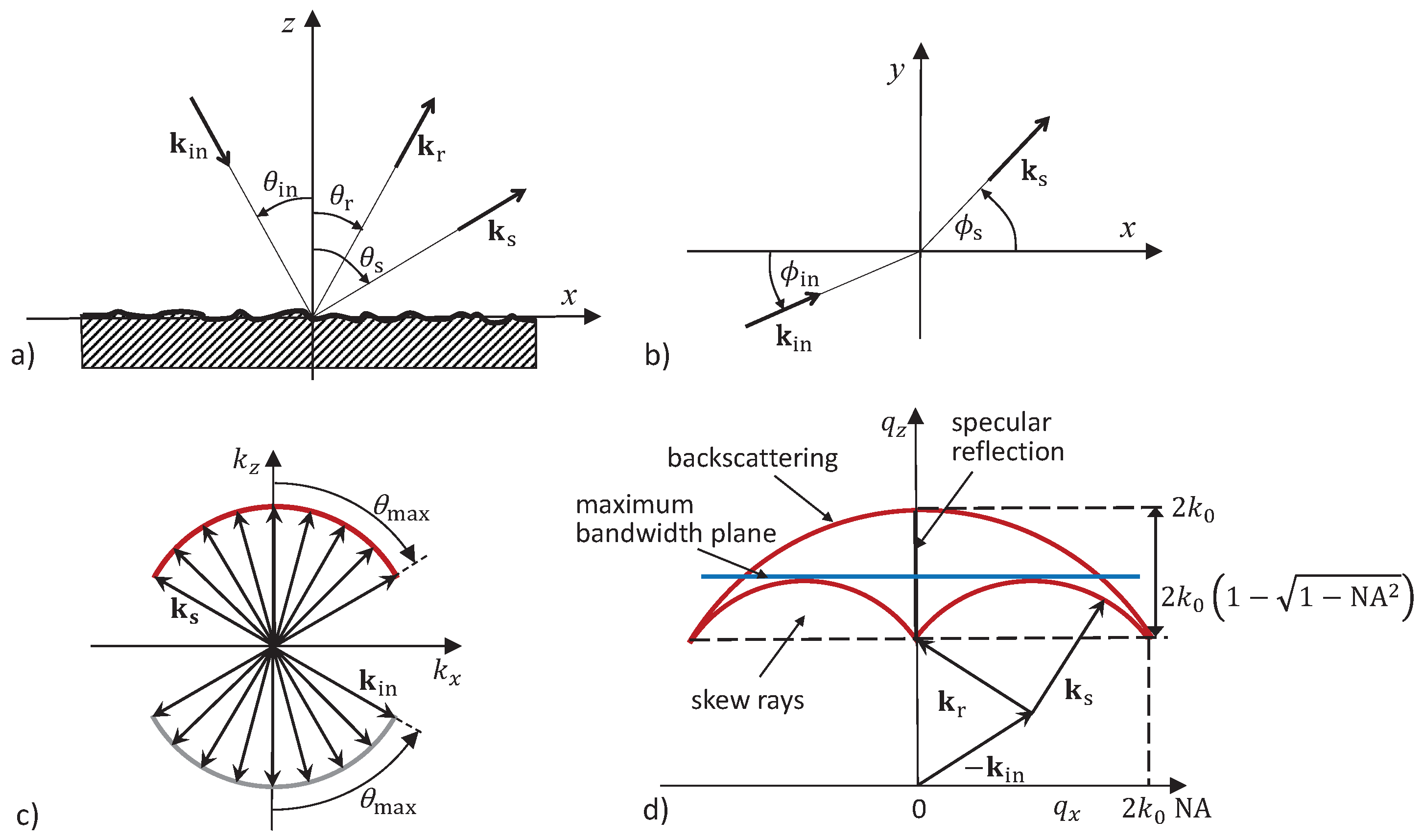
In order to quantify these effects, we briefly summarize the Kirchhoff formulation of [11,15,17] with respect to the scattering geometry of a microscope in reflection mode as already published in our previous paper [6]. For simplicity, we assume a perfectly reflecting surface and a monochromatic plane wave of wavelength and wavenumber . According to Figure 1a, is the angle of incidence with respect to the z-axis and the angle, the -component of the incident wave vector includes with the x-axis (see Figure 1b). For an incident plane wave characterized by and , the normalized scattered far-field under the azimuthal angle and the scattering angle according to Figure 1a,b results from the integration:
where
and the area A of integration corresponds to the field of view of the microscope. For a surface, which is rough in the x-direction only, i.e., , is given by
where the angle depends on the scattering angle . The wave vector shown in Figure 1a holds for specular reflection from a plane mirror in the -plane, i.e., .
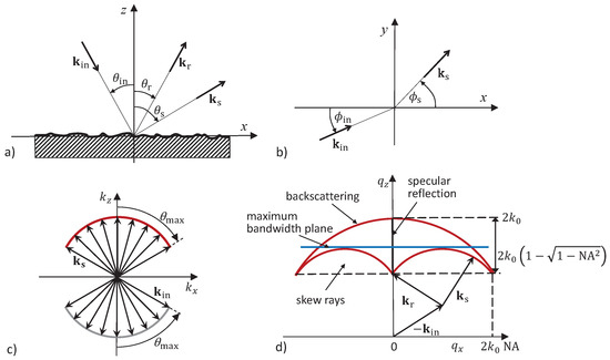
Figure 1.
Scattering geometry [6] (a) in the -plane; (b) in the -plane; (c) Ewald sphere construction for a reflection-type microscope assuming plane wave illumination incident under an angle taking all angles of incidence and all scattering angles that are covered by the objective’s NA into account; (d) Ewald limiting sphere construction showing the vertical line corresponding to specular reflection, an outer sphere of radius and an axial low-frequency limit given by . The blue line represents the maximum transverse spatial frequency bandwidth along the axis at a certain value.
Since a transfer function is defined as the system’s response with respect to a single point scatterer represented by a 3D -function , determining the transfer characteristics of a CSI instrument assumes a spherical wave propagating from a (virtual) point source in the measurement arm for each reflected plane wave in the reference arm of the CSI instrument [2,7,8,19].
Due to the symmetry of a microscope objective lens, the 3D transfer function shows rotational symmetry with respect to the -axis. Thus, replacing the coordinates and by the new coordinate results in:
As according to (9) no longer depends on or , any cross section including the -axis represents the complete TF. In the backscatter direction, equals , and thus .
2. Results
2.1. Derivation of the 3D Transfer Function for Monochromatic Light
With respect to the following derivation, we refer to our paper [19] using the Ewald or McCutchen sphere construction according to Figure 1c [7,13] considering that the angles of incidence and the scattering angles are limited by the NA of the microscope objective. The side view of the resulting Ewald limiting sphere (Figure 1) represents the cut-off in the spatial frequency domain due to the NA of the objective lens [12,21,24].
For the calculation of the 2D MTF, two uniformly-filled circular apertures are correlated [20]. The generalized physical situation is explained by Figure 2, where the incident and the scattered wave vectors form spherical caps of radius (see Figure 2a. The NA limits the lateral extension of these caps, which are inverted with respect to each other as shown in Figure 1c because of the different propagation direction of the incident and scattered waves with respect to the optical axis of the objective lens. The lateral and vertical shift of the caps represents the lateral and the axial spatial frequency, respectively. Under the assumption that the caps must intersect, the maximum axial shift is , whereas the minimum axial shift equals (see Figure 1c and Figure 2a). Contributions of the lateral spatial frequency components to the imaging process can be expected as long as . Integration along the -axis results in the sum of the areas and area , which equals the intersection area of two laterally shifted circular apertures (see Figure 2c). results via integration from to . The corresponding lines of intersection of the two caps are full circles tilted by the angle (see Figure 2b). Hence, area resulting from integration is an ellipse (see Figure 2c). Area is attributed to the integration range from to and represents the difference between the intersecting area of the two circles and . The areas and used to obtain the 3D TF are related to and by
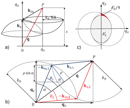
Figure 2.
Geometry for the derivation of the 3D TF according to [19]: (a) two spherical caps corresponding to wave vectors of incident waves and scattered waves are correlated. The point P is defined by vector with coordinates and in the spatial frequency domain representing the shift of the centres of the two spheres of radius ; (b) the circle of intersection of the two spheres is characterized by the radius and the tilt angle . The vectors , , , and corresponding to point P are located in the plane of incidence (-plane); (c) top view representing the area for height shifts between and as well as area for height shifts between and .
As shown in Figure 2b, area is given by a circle of radius . In the -plane, the points of intersection of circles of radius centered around the origin and point P are the end points of the two vectors and and the starting points of the vectors and . These vectors exhibit that each point P of the TF can be reached by two different ray paths in the -plane as described by Quartel and Sheppard [16]. Due to the symmetry of the configuration,
where The angle is given by
In order to calculate the 3D TF related to a point scatterer, we used the derivations and [19]. According to the projection slice theorem [25], this leads to the familiar MTF formula for a diffraction limited system by -integration. Here, we are interested in the transfer function that holds for specularly reflective surfaces. In the ideal case, according to energy conservation, the light reflected or diffracted at a specular surface hitting the open aperture of the objective lens will contribute to the measured signal without loss of energy. Under this assumption for a certain value, the 3D TF should no longer depend on the coordinate. This is achieved if the multiplication by is renounced and the derivations and are used to define the 3D TF. As a consequence, the intensity distribution of the reflected and diffracted light in the pupil plane is no longer uniform. According to Figure 2b, is given by
and, therefore,
where the negative sign agrees with the fact that the circle of the largest radius is assigned to the smallest -value.
The contribution to the TF coming from the area originates from skew rays [17], the wave vectors of which leave the plane of incidence (-plane). Consistent with [19], the derivation of with respect to results in
Hence, the desired formula for the 3D transfer function is:
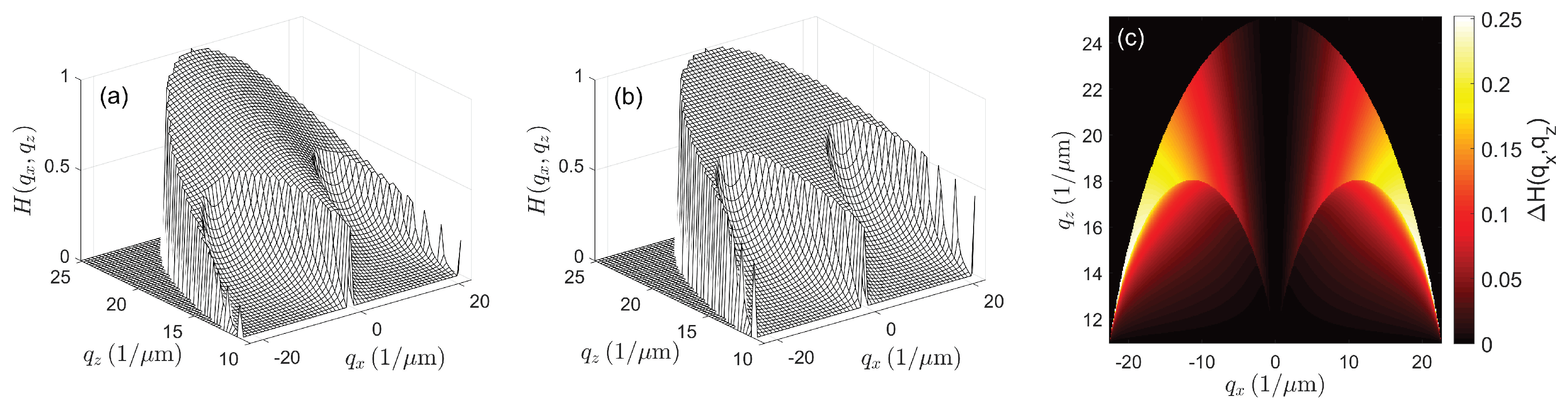
where and are given by (14) and (15). This result is in agreement with earlier calculations of interference signals arising from perfectly adjusted perfect mirrors, i.e., for [26,27]. In the following, is normalized to a maximum value of . The dependency on in the argument indicates that is the 3D TF for the monochromatic case, where (16) is an analytical formula that calculates the 3D TF for specularly reflective and diffractive surfaces, comprising often used calibration standards in CSI. The differences between the 3D TFs obtained in [19] for scattering surfaces and the 3D TFs according to (16) are shown in Figure 3 and Figure 4 for a wavelength of 500 nm and an NA of 0.55 (Figure 3) as well as 0.9 (Figure 4). Note that, due to the rotational symmetry with respect to the -axis, the results presented in this paper are cross sections of in the -plane. In the paraxial case, i.e., for small NA values, the differences between the TFs for specular reflection and scattering will be negligible. However, for an NA of 0.9, differences of up to 0.25 appear. The deviations between the results can be explained by the different scattering behaviour in the two situations, which is well known from confocal microscopy [21] (Chapter 1), [22] (Chapter 3). For the point scatterer, a constant intensity distribution of the scattered light is assumed to appear in the pupil plane of the objective lens. This leads to a scattering characteristic, which is similar to a Lambertian emitter, i.e., for a constant , the scattered light intensity is maximum in the direction of reflection () and falls down continuously until the backscattering direction () is reached. This can be obtained from the factor according to (12), which represents the major difference in the calculation of the TF for a point scatterer and a specular surface. Equation (12) can be rewritten as:
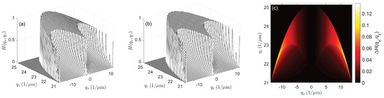
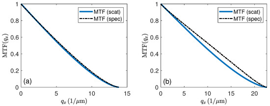
Figure 3.
3D representations of cross sections of the transfer functions for and nm: (a) for scattering objects; (b) for specularly reflecting objects; and (c) cross sectional view of the difference between (b) and (a).
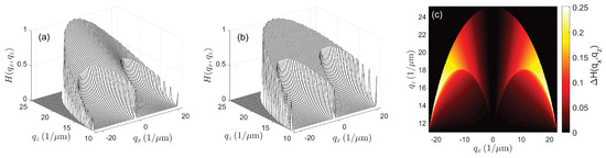
Figure 4.
3D representations of cross sections of the transfer functions for and nm: (a) for scattering objects; (b) for specularly reflecting objects; and (c) cross sectional view of the difference between (b) and (a).
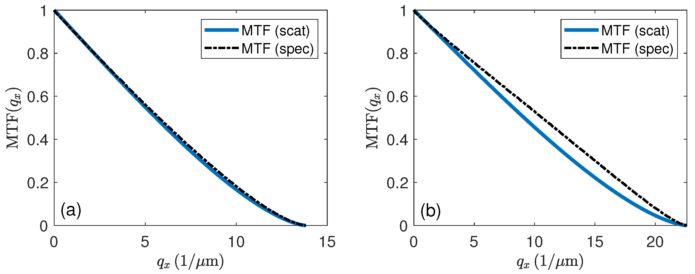
On the other hand, the irradiance of reflected light incident on a perfect mirror under an angle must be the same whether the mirror is perfectly aligned in the -plane or if it is tilted by an angle such that the plane wave is incident normal to the surface. This is achieved by (14), which no longer depends on the coordinate. The 3D TF discussed so far holds for conventional microscopes. Therefore, it should be mentioned that, due to the symmetry of the arrangement according to Figure 2a,b and the uniform pupil illumination, it equals the 3D TF of an interference microscope [6,19]. As a consequence of the different 3D TFs shown in Figure 3 and Figure 4, the MTFs also resulting from -integration will be different as Figure 5 confirms. For the point scatterer, the MTF exactly agrees with the MTF of a diffraction limited system [19], whereas in the specular case at high NA values, the resulting MTF comes closer to a linear function (see Figure 5b). Additionally, note that the plateau of for enables the perfect reconstruction of the weak phase grating as long as
which is the Abbe criterion of lateral resolution.
2.2. Dependence of 3D Transfer Functions on Temporal Coherence
The results for monochromatic illumination shown so far can be easily extended to the case of broadband illumination if the spectral distribution of the light source and the spectral sensitivity of the optical system including the camera is considered for the calculation of the 3D TF by
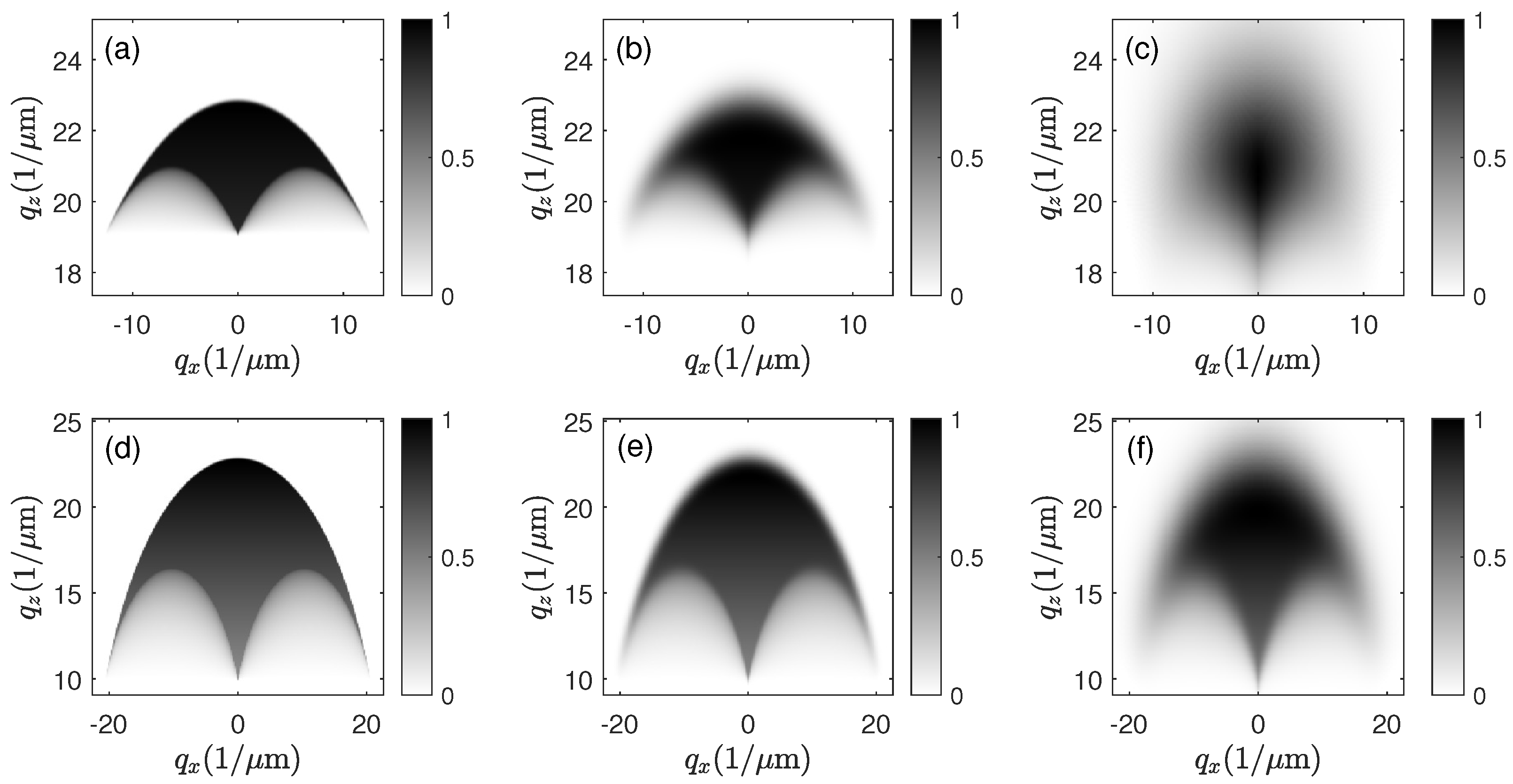
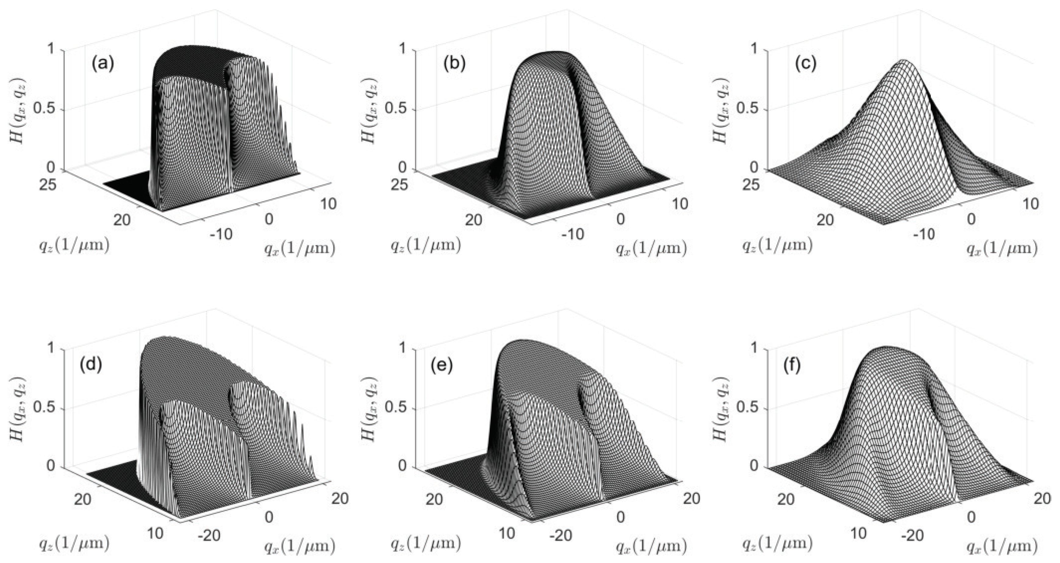
where . With respect to the transfer function , it should be noticed that all Cartesian axes in -space scale with the wavenumber . As a consequence, the ’wings’ of the transfer function at high and low -values will be significantly shifted if the wavenumber changes. This is shown in Figure 6 for two series of TFs. Figure 6a–c are related to an NA of 0.55 and a center wavelength of 550 nm. The spectral distribution obeys a Gaussian wavenumber distribution. From Figure 6a–c, the spectral FWHM bandwidth as a function of the wavelength of light increases from 2.5 nm (a) to 25 nm (b) and 100 nm (c). Figure 6d–f show the same for an NA of 0.9. With respect to practical applications of CSI, a central wavelength of 550 nm is chosen. Instead of the wavelength of 500 nm according to Figure 3 and Figure 4, 550 nm is a realistic value even if the FWHM equals 100 nm. In both cases shown in Figure 6, with increasing spectral bandwidth, the transfer functions look more and more blurred. 3D representations of the cross sections of the same transfer functions are depicted in Figure 7. These exhibit that the size of the plateau in the center of the 3D TF decreases as the spectral bandwidth increases. In Figure 7c for NA = 0.55 and FWHM = 100 nm, the plateau-like area is no longer visible.

Figure 6.
Cross sectional views of the transfer functions : (a–c) for , nm and spectral FWHM of 2.5 nm (a); 25 nm (b); and 100 nm (c); (d–f) for , nm and spectral FWHM of 2.5 nm (d); 25 nm (e); and 100 nm (f).
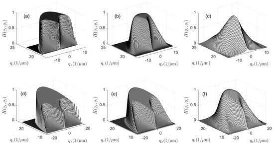
Figure 7.
3D representations of cross sections of the transfer functions according to Figure 6: (a–c) for , nm and spectral FWHM of 2.5 nm (a); 25 nm (b); and 100 nm (c); (d–f) for , nm and spectral FWHM of 2.5 nm (d); 25 nm (e); and 100 nm (f).
2.3. 3D Transfer Functions and Surface Topography Reconstruction
This section is intended to investigate the impact of the shape of the 3D TF of an interference microscope on the related surface topography reconstruction capabilities. Recent publications by different researchers elucidating this subject [5,7,10,28] come to the conclusion that, for the case of a uniformly-filled illumination pupil and sufficiently small surface height deviations, the transfer function of a CSI instrument takes the form of the familiar modulation transfer function (MTF) given by the autocorrelation function of a circular pupil [20]. In our nomenclature, this means that, in order to obtain the CSI measurement result in the spatial frequency domain, for a certain axial spatial frequency value, the scattered field would be multiplied by the 2D MTF, which depends solely on the coordinate defined in (9) due to the rotational symmetry. However, according to the above sections, our results differ with respect to the following two points:
- The 2D MTF can be derived from the 3D TF via integration with respect to the coordinate [19]. Expressing the 2D MTF by an autocorrelation of a uniformly-filled 2D circular pupil function assumes that both the illumination as well as the imaging pupil plane is uniformly-filled. As discussed before, this requires single point scatterers with certain scattering characteristics on the surface under investigation. In contrast, specularly reflecting surfaces such as typical surface standards lead to a non-uniformly filled image pupil function even if the illumination pupil is uniformly-filled (see Figure 5).
- The stack of interference images resulting from a CSI measurement can be analyzed at certain axial spatial frequencies. According to [5,10], this analysis is typically performed for the so-called equivalent wavelength , which corresponds to the axial spatial frequency value . As a consequence, not the integration of with respect to plays a crucial role for surface reconstruction but the coarse of the function for a certain constant -value. This value is related to what we call the ‘evaluation wavelength’ byNote that may equal the equivalent wavelength or not.
Sheppard and Larkin [26] introduce the -factor
for an aplanatic system with uniformly filled pupils. This NA-factor describes the increasing fringe spacing depending on the NA of the optical system and, therefore, it can be used to define the equivalent wavelength by
or the equivalent axial spatial frequency
Equation (20) can be derived as the center of gravity of the transfer function i.e.,
In practical applications of CSI, the evaluation wavelength is mostly chosen such that . A slightly different alternative is to choose an evaluation wavelength
which corresponds to a maximum bandwidth of the corresponding partial transfer function (see the blue line in Figure 1d). This results in
If maximum lateral resolution is required, the evaluation wavelength should be chosen such that
as marked by the dashed black line in Figure 1d. The three functions , , and are plotted in Figure 8.
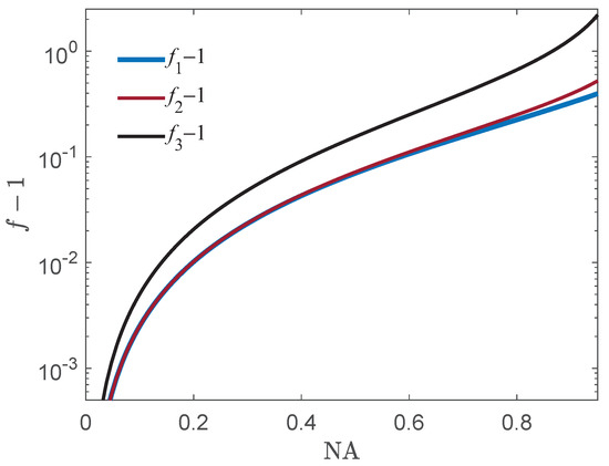
Figure 8.
Numerical aperture factors: is related to the equivalent wavelength, corresponds to the maximum bandwidth wavelength, and to the maximum effective wavelength.
Once the evaluation wavelength is chosen, the corresponding partial transfer function is calculated and multiplied by the Fourier transformed phase object resulting in the filtered Fourier transformed phase object
Fourier transform with respect to the transverse coordinates leads to the filtered phase object
from which the reconstructed surface profile surface can be obtained by
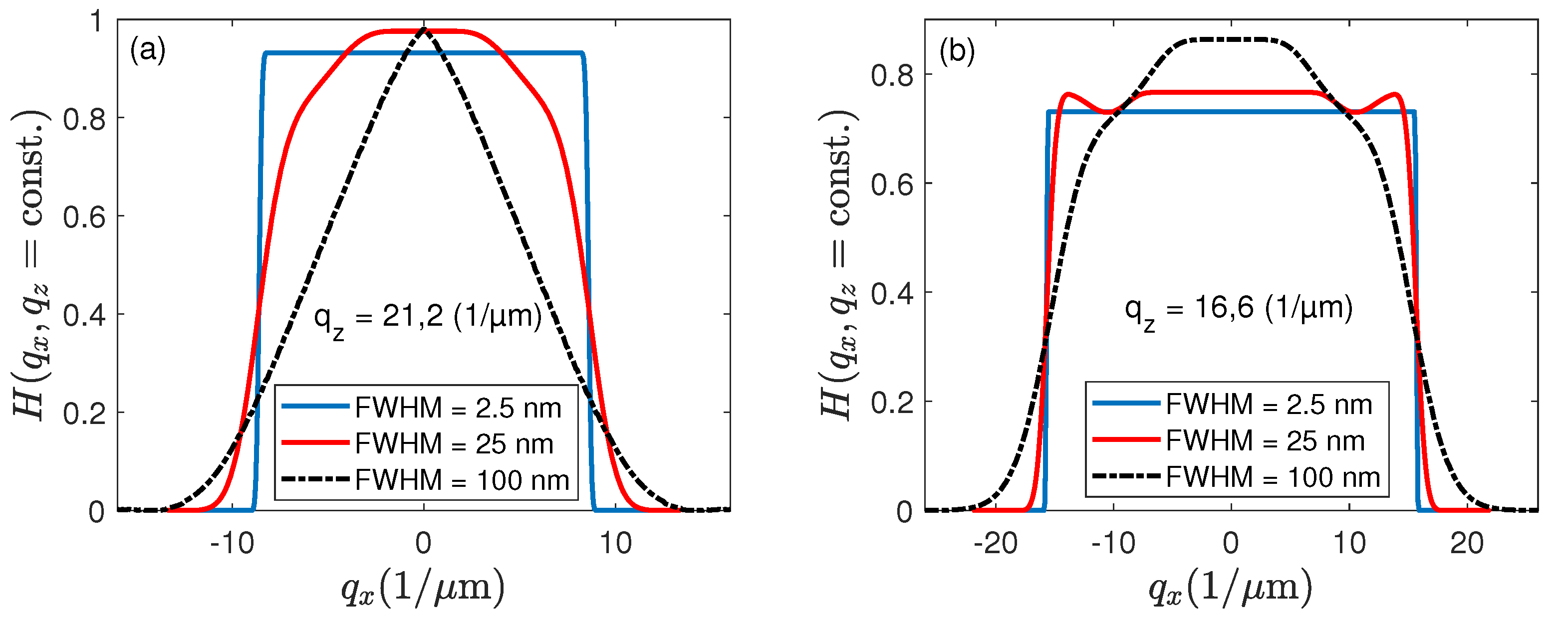
where represents the imaginary part and the real part. Figure 9 depicts cross sectional views of the 3D TFs according to Figure 6 and Figure 7 for NA = 0.55 and µ (Figure 9a) as well as for NA = 0.9 and µ (Figure 9b). Note that the values of are chosen slightly higher than . Thus, shows a plateau even for spectral distributions of slightly broader FWHM. For the lower NA, the cross sectional views in Figure 9a exhibit a strong dependence on the spectral FWHM, whereas, in Figure 9b, the changes are less significant.
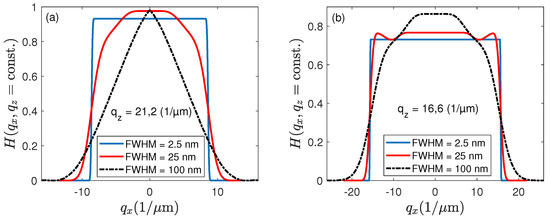
Figure 9.
Cross sectional views of the transfer functions for different spectral bandwidth given by the FWHM, (a) for , nm, and , (b) for , nm, and .
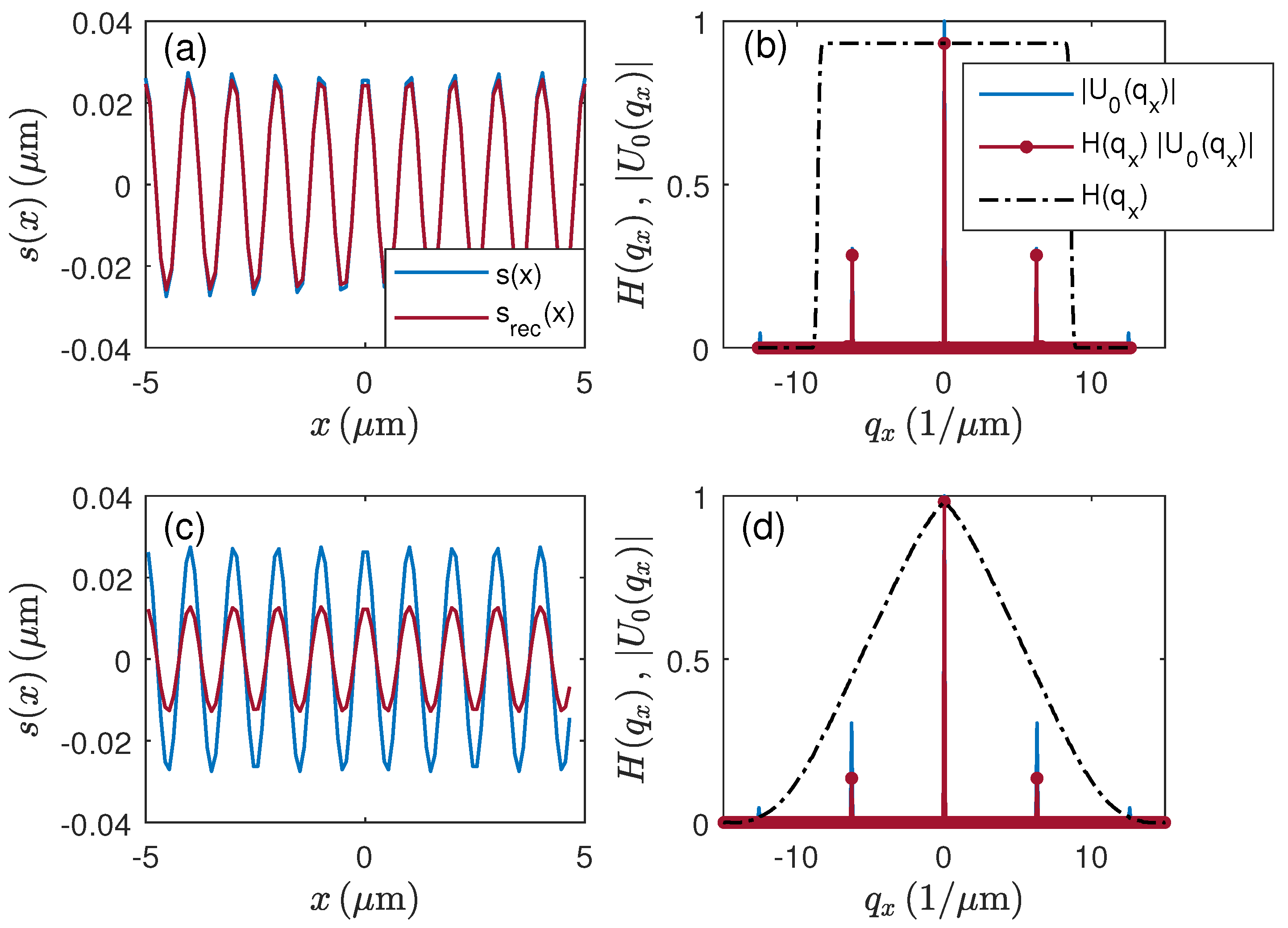
Figure 10a shows the surface profile and the reconstructed surface profile of a cosine-shaped surface according to (2) of nm peak-to-valley (PV) amplitude and 0.5 µm period length. For the corresponding phase object (1) represents a satisfactory approximation. The absolute value of the Fourier transform of with respect to the x coordinate (see (5)) is displayed in Figure 10b together with the partial transfer function for µ and an FWHM of 2.5 nm (see Figure 9a) as well as the product Due to the rectangular shape of the reconstructed profile shows only slight amplitude deviations caused by higher diffraction orders which are not considered in the reconstruction. For Figure 10c,d, the same profile and evaluation wavelength but an FWHM of 100 nm (see Figure 9a) is presumed. Since the value of the partial transfer function is below 0.5 at the -position of the spatial frequency of the surface, the amplitude of the reconstructed surface profile is less than half of the original amplitude too.

Figure 10.
Surface profile reconstruction using the transfer function for and nm: (a,c) cosinusoidal input profile of 0.5 µm period length and 55 nm PV-amplitude and reconstructed profiles ; (b,d) corresponding partial transfer functions for µ, absolute value of the electric field and product , (a,b) for FWHM = 2.5 nm, (c,d) for FWHM = 100 nm.
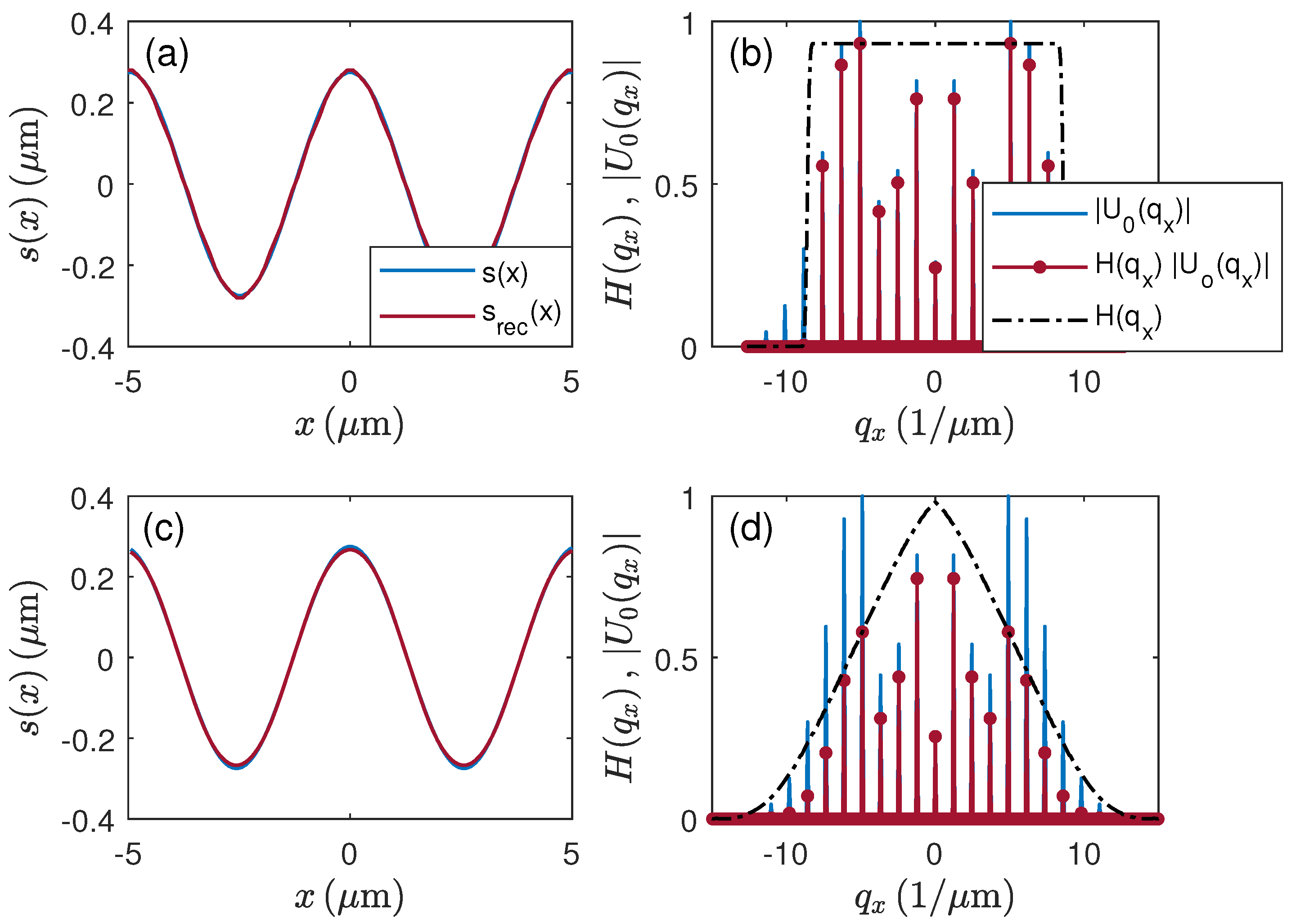
Figure 11 shows surface profiles and reconstructed surface profiles of a cosine-shaped surface of 550 nm peak-to-valley (PV) amplitude and 5 µm period length. In this case, the corresponding Fourier transformed phase object comprises numerous diffraction orders as it can be seen in Figure 11b,d. In Figure 11b, for an FWHM of 2.5 nm, higher order spatial frequency contributions are cut by the corresponding partial transfer function for µ. For the broader spectral bandwidth according to Figure 11d, corresponding to an FWHM of 100 nm, the higher order diffraction maxima are damped down significantly. However, in both cases, the reconstructed profiles agree quite well with the original input profiles (see Figure 11a,c).
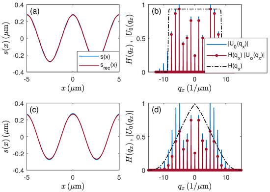
Figure 11.
Surface profile reconstruction using the transfer function for and nm: (a,c) cosinusoidal input profile of 5 µm period length and 550 nm PV-amplitude and reconstructed profiles ; (b,d) corresponding partial transfer functions for µ, absolute value of the electric field and product , (a,b) for FWHM = 2.5 nm, (c,d) for FWHM = 100 nm.
In Figure 12, an input profile with 50 nm PV-amplitude and 0.3 µm period length is presumed. This period is close to the resolution limit of 0.28 µm for NA = 0.9 and nm. According to Figure 12a for µ, the first order diffraction component is cut by the corresponding partial TF in Figure 12b, such that the cosinusoidal structure does not appear in the reconstructed profile. However, if is reduced to 13.0 µ (Figure 12c,d), the bandwidth of the partial TF increases and the cosinusoidal structure is resolved, although the PV-amplitude is reduced approximately by a factor of 3. This is in accordance with our experimental results published earlier [6,29].
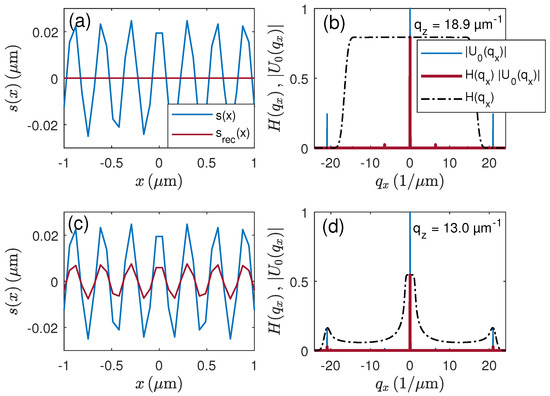
Figure 12.
Surface profile reconstruction using the transfer function for and nm: (a,c) cosinusoidal input profile of 0.3 µm period length and 50 nm PV-amplitude and reconstructed profiles (b,d) partial transfer functions for FWHM = 25 nm, absolute value of the electric field and product , (a,b) for µ, (c,d) for µ.
All results of surface profile reconstruction shown so far are based on the analysis of the phase of the corresponding interference signals at the certain wavelength . However, in practical applications, CSI signal processing is usually a combination of coherence peak detection and phase analysis [30,31,32]. Since the 3D TF is defined in the 3D spatial frequency domain, it is obvious to determine the maximum position of the signal envelope in the spatial frequency domain, too. As pointed out by de Groot and Deck [30], the envelope’s position equals the derivative of the phase with respect to the axial spatial frequency Considering (1) and (2), the phase of
results in
Thus, the surface topography can be reconstructed by:
where is an infinitesimal increment with respect to the coordinate.
In order to obtain the envelope position in the spatial frequency domain, we first define based on (5)
and
Then, the derivative of the phase function is calculated numerically and the reconstructed surface profile called coherence profile results in:
Note that and are normalized such that as long as and as long as . Under these assumptions, .
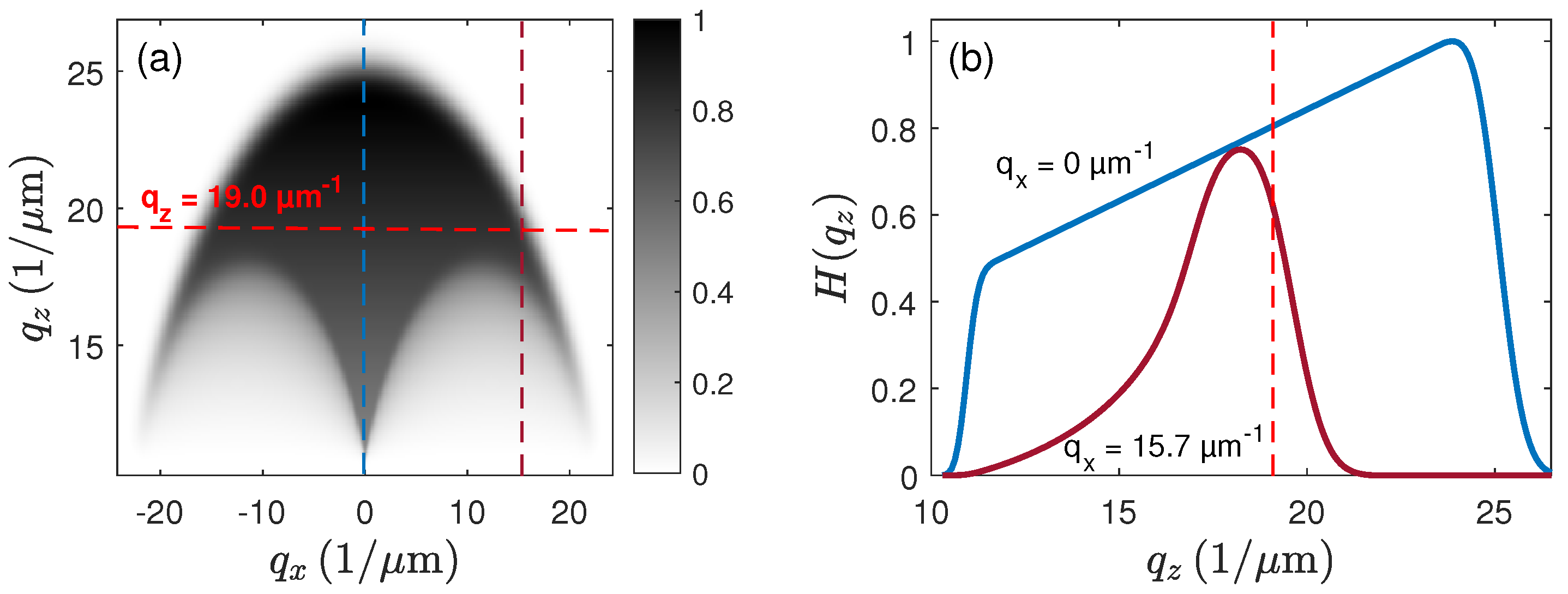
Since (34) contains the difference of the electric fields depending on at and , we can describe the influence of the instrument by the use of the envelope transfer function defined as the normalized difference quotient
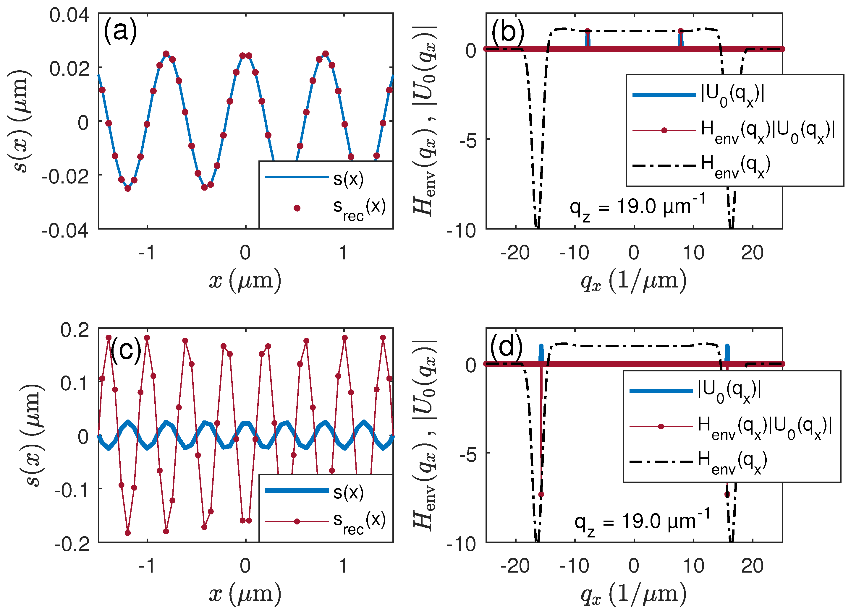
where As long as , the reconstructed coherence profile equals the original profile, i.e., . Unfortunately, the function no longer shows a simple low-pass filter characteristic and thus the results of envelope and phase evaluation may be different. The occurring problem is explained by Figure 13, which shows and cross sections of for constant values of µ and µ belonging to the real and the imaginary part of . The horizontal dashed red line in Figure 13a and the vertical dashed red line in (b) correspond to µ. Equation (35) results in the normalized derivative of with respect to at . Figure 13b shows that is positive for µ, whereas it is negative with a much higher gradient for µ. As a consequence, the transfer function according to Figure 14b,d results, which leads to the reconstructed coherence profiles in Figure 14a,c depending on the period of the input surface. Due to the large absolute value and the negative sign of for µ, the reconstructed profile in Figure 14c is inverted and the amplitude is approximately seven times the amplitude of the original profile. This effect has already been obtained from experimental investigations [33]. If the period of the surface is doubled (i.e., µm), the evaluation of the coherence peak position results in Figure 14a,b. In this case, the reconstructed profile perfectly agrees with the original profile.
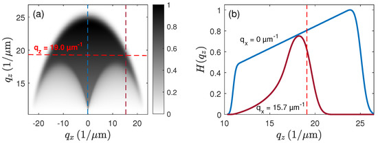
Figure 13.
(a) Cross sectional view of the transfer function for , nm and FWHM of 25 nm, (b) for (blue line) and = 15.7 (red line).
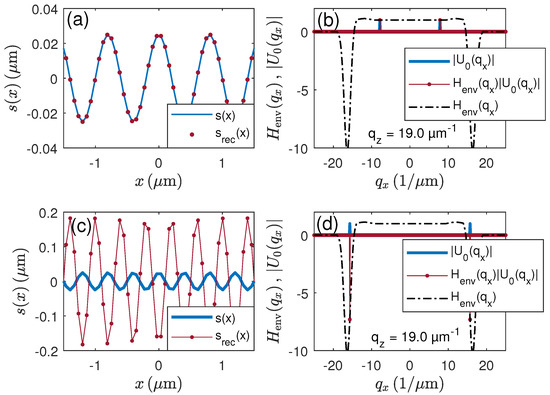
Figure 14.
Surface profile reconstruction by coherence peak detection using the transfer function for and nm: (a) cosinusoidal input profile of 0.8 µm period length and 50 nm PV-amplitude and reconstructed coherence profile ; (b) partial transfer function for and FWHM = 25 nm, absolute value of the electric field and ; (c) cosinusoidal input profile of 0.4 µm period length and 50 nm PV-amplitude and reconstructed coherence profile ; (d) same corresponding partial transfer function , absolute value of the electric field and .
Note that the enhancement-effect of high-frequency contributions depends on the coherence length of the contributing light. Furthermore, the NA of the system affects its extension along the -axis. It should be mentioned that the same phenomenon appears at higher surface slopes, where the reflected light is attributed to higher transverse spatial frequency contributions [6,9,34,35,36]. Furthermore, the effect hardly depends on whether the 3D TF of a specular surface or a point scatterer is presumed to be valid.
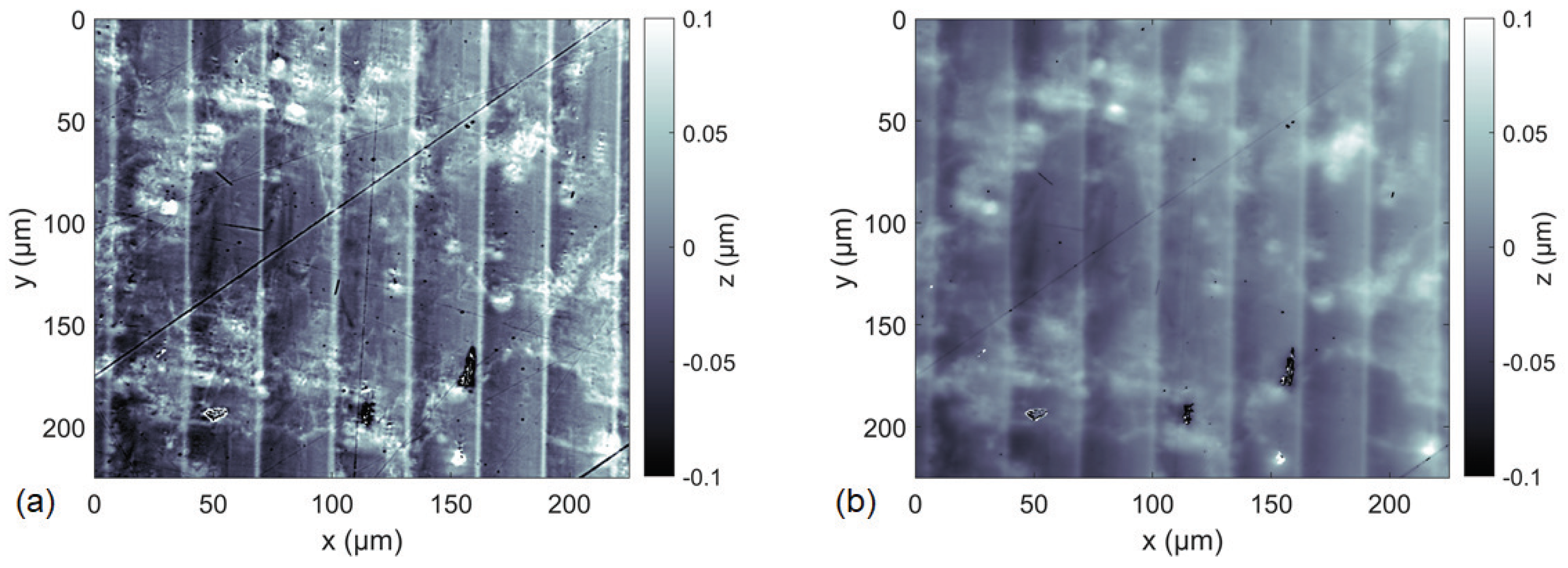
As a final example, Figure 15 shows the measured topography of a diamond milled aluminum mirror as a real-world object. The comparison of the results of envelope analysis in Figure 15a and phase analysis in (b) exhibits that the envelope result is characterized by high-frequency components, whereas the result of phase evaluation appears to be low-pass filtered. We suppose that this is a consequence of the high spatial frequency enhancement introduced in Figure 13 and Figure 14. However, since the NA is 0.55 in Figure 15, the bandwidth for high-frequency enhancement is even broader in this case. In both cases, the sawtooth-like grooves of approximately 50 nm depth originating from the manufacturing process can be recognized. Although the theoretical derivation of the 3D TF reported in Section 2.1 neglects the central obscuration due to the reference mirror in a Mirau interferometer, the results according to Figure 15 confirm the basic effect of different spatial frequency transfer characteristics depending on whether the coherence or the phase profile is analyzed.

Figure 15.
Measured 3D topographies of a diamond milled aluminum mirror using a Mirau CSI with NA = 0.55, a red LED with a central wavelength of 630 nm for illumination and an evaluation wavelength of 670 nm, (a) result of envelope evaluation; (b) result of phase evaluation.
3. Discussion
This work uses a previously introduced CSI model called the double foil model, which is a combination of both Kirchhoff’s diffraction theory and Abbe’s theory of image formation in a microscope. According to this model, both the surface of the object under investigation as well as the reference mirror of the interferometer are treated either based on the foil model or, equivalently, as a phase object. The light scattering process assuming spatially incoherent Köhler illumination is described by the use of an Ewald sphere allowing for determining the transfer function of a CSI instrument depending on its numerical aperture. In addition, we introduced a mostly analytical computation method to calculate the 3D TF of a microscope in reflection mode under the assumption that the object under investigation can be described by single point scatterers. This transfer function agrees with the 3D TF of an interference microscope under the same assumption, namely that the surface under investigation consists of point scatterers.
Based on these fundamentals, we derive an analytical formula that calculates the 3D TF for specular surfaces, which typically needs to be considered if calibration surfaces are being measured. The procedure is similar to the calculation introduced in context with the 3D TF for point scatterers. However, the results are different. Consequently, the transfer function of an instrument depends on whether the surface under investigation is represented by point scatterers or by specular reflection. Since the 3D TF mentioned above holds for monochromatic light only, we additionally study the consequences of limited temporal coherence considering the spectral bandwidth of the light source. It turns out that transfer characteristics and, therefore, the surface reconstruction capabilities in CSI strongly depend on the spectral bandwidth of the light source and the spectral sensitivity of the optical system. The surface of a weak phase object can be reconstructed by use of a partial transfer function, which equals a cross section of the 3D TF for a certain axial spatial frequency value . In this context, it should be mentioned that most commercial CSI instruments use spectrally broadband light sources such as white-light LEDs or tungsten lamps. However, the results shown here demonstrate that, for medium and high NA systems, light sources of smaller spectral bandwidth sometimes provide a better lateral resolution.
Finally, we show that, for certain transverse spatial frequencies of a periodic surface, the results obtained by CSI measurements will significantly differ, depending on whether the phase or the envelope of the interference signals recorded by individual camera pixels is being analyzed, resulting either in the phase or in the coherence profile. In an extreme case, the coherence profile obtained from the envelope will be inverted and show much higher amplitudes compared to the original surface. Strong deviations between the real surface profile and the measured coherence profile also appear at steeper surface slopes, where the corresponding transverse spatial frequency contributions are located at higher values, such that the envelope of the interference signals shifts due to changes of the envelope transfer function introduced in Section 2.3. In contrast, the profiles obtained from the phase show no inversion but possibly a reduced amplitude due to the low-pass filter characteristic of the TF. This effect can also be recognized in a measurement result taken from a precision manufactured metallic mirror.
4. Materials and Methods
The results presented in this paper primarily follow from the theoretical considerations of Section 2. The corresponding formulae are either derived in this paper or are taken from the references mentioned. Computations are conducted and diagrams are plotted using Matlab software.
The experimental results shown in Figure 15 are obtained with a home-build CSI instrument equipped with a Nikon CF IC EPI Plan DI 50x objective lens.
5. Conclusions
In this contribution, three-dimensional transfer functions of CSI instruments are derived and analyzed. The effects introduced and discussed especially appear in CSI systems of higher numerical aperture, where the paraxial approximation no longer holds. Such instruments are needed if high lateral resolution in the sub-micrometer range is required. It is shown that, in contrast to usual assumptions, the three-dimensional transfer function depends not only on instrumental characteristics but also on the surface under investigation. Different transfer functions apply if the object’s surface can be characterized by single point scatterers or by specular reflection and diffraction. This is physically evident, since, as long as the reflected or diffracted light from a perfectly reflecting surface is collected by the objective lens, no radiation energy is lost, whereas single scatterers on a surface always lead to a loss of the incident radiation energy. For small numerical apertures, fulfilling the paraxial approximation the 3D transfer function can be simply approximated by the value of one within the transfer range of the system, independently on whether the surface can be characterized by reflection, diffraction or scattering.
In addition, the three-dimensional transfer behavior of CSI instruments strongly depends on the spectral bandwidth of the light source and the camera. In certain cases, a narrow spectral bandwidth is advantageous regarding the lateral resolution of the instrument. In addition, systematic deviations appear if either the position of the coherence envelope or the phase of a CSI signal is used for the topography reconstruction. A detailed analysis of the three-dimensional transfer function reveals that, for the effective wavelengths, which are typically used in CSI signal processing, the surface topography obtained via phase evaluation of the interference signals is generally accompanied by an optical low-pass filtering of the spatial frequency contributions of the surface. In contrast, the topography derived from the coherence peak or envelope position of an interference signal may lead to enhanced higher spatial frequency surface components in the measured topography data. Thus, the results presented in this paper provide detailed insight into the transfer behavior of CSI instruments and help to better understand the resulting physical phenomena. Furthermore, they may contribute to building more realistic virtual instruments and estimating the uncertainty of a certain measurement result. Finally, the findings presented in this contribution enable extending the signal analysis strategy of CSI systems in order to fully access the measurement capabilities of a given interferometer system.
Author Contributions
Conceptualization, P.L.; methodology, P.L.; software, P.L.; mathematical validation, T.P.; formal analysis, P.L.; investigation, P.L.; writing, P.L.; proof reading, T.P. and S.H.; experimental setup and measurement, S.H. All authors have read and agreed to the published version of the manuscript.
Funding
This research work was partially funded by the EMPIR program (project TracOptic, 20IND07) co-financed by the European Union’s Horizon 2020 research and innovation program.
Institutional Review Board Statement
Not applicable.
Informed Consent Statement
Not applicable.
Data Availability Statement
The data obtained and used in this contribution can be provided by the corresponding author upon request.
Conflicts of Interest
The authors declare no conflict of interest.
References
- Malacara, D. (Ed.) Optical Shop Testing; John Wiley & Sons: Hoboken, NJ, USA, 2007. [Google Scholar]
- Coupland, J.; Lobera, J. Holography, tomography and 3D microscopy as linear filtering operations. Meas. Sci. Technol. 2008, 19, 074012. [Google Scholar] [CrossRef] [Green Version]
- Coupland, J.; Mandal, R.; Palodhi, K.; Leach, R. Coherence scanning interferometry: Linear theory of surface measurement. Appl. Opt. 2013, 52, 3662–3670. [Google Scholar] [CrossRef] [Green Version]
- Su, R.; Thomas, M.; Liu, M.; Drs, J.; Bellouard, Y.; Pruss, C.; Coupland, J.; Leach, R. Lens aberration compensation in interference microscopy. Opt. Lasers Eng. 2020, 128, 106015. [Google Scholar] [CrossRef]
- de Groot, P.; Colonna de Lega, X. Fourier optics modeling of interference microscopes. J. Opt. Soc. Am. A 2020, 37, B1–B10. [Google Scholar] [CrossRef] [PubMed]
- Lehmann, P.; Künne, M.; Pahl, T. Analysis of interference microscopy in the spatial frequency domain. IOP J. Phys. Photonics 2021, 3, 014006. [Google Scholar] [CrossRef]
- Su, R.; Coupland, J.; Sheppard, C.; Leach, R. Scattering and three-dimensional imaging in surface topography measuring interference microscopy. J. Opt. Soc. Am. A 2021, 38, A27–A41. [Google Scholar] [CrossRef]
- Pahl, T.; Hagemeier, S.; Künne, M.; Danzglock, C.; Reinhold, N.; Schulze, R.; Siebert, M.; Lehmann, P. Vectorial 3D modeling of coherence scanning interferometry. Proc. SPIE 2021, 11783, 117830G. [Google Scholar]
- Künne, M.; Pahl, T.; Lehmann, P. Spatial-frequency domain representation of interferogram formation in coherence scanning interferometry. Proc. SPIE 2021, 11782, 117820T. [Google Scholar]
- de Groot, P.; Colonna de Lega, X.; Su, R.; Coupland, J.; Leach, R. Fourier optics modelling of coherence scanning interferometers. Proc. SPIE 2021, 11817, 118170M. [Google Scholar]
- Beckmann, P.; Spizzichino, A. The Scattering of Electromagnetic Waves from Rough Surfaces; Artech House, Inc.: Norwood, MA, USA, 1987. [Google Scholar]
- Born, M.; Wolf, E. Principles of Optics: Electromagnetic Theory of Propagation, Interference and Diffraction of Light; Cambridge University Press: Cambridge, UK, 2013. [Google Scholar]
- McCutchen, C.W. Generalized aperture and the three-dimensional diffraction image. J. Opt. Soc. Am. 1964, 54, 240–244. [Google Scholar] [CrossRef]
- Wombell, R.J.; DeSanto, J.A. Reconstruction of rough-surface profiles with the Kirchhoff approximation. J. Opt. Soc. Am. A 1991, 8, 1892–1897. [Google Scholar] [CrossRef]
- Sheppard, C.; Connolly, T.; Gu, M. Imaging and reconstruction for rough surface scattering in the Kirchhoff approximation by confocal microscopy. J. Mod. Opt. 1993, 40, 2407–2421. [Google Scholar] [CrossRef]
- Quartel, J.C.; Sheppard, C.J.R. Surface reconstruction using an algorithm based on confocal imaging. J. Mod. Opt. 1996, 43, 469–486. [Google Scholar] [CrossRef]
- Sheppard, C. Imaging of random surfaces and inverse scattering in the Kirchoff approximation. Waves Random Media 1998, 8, 53–66. [Google Scholar] [CrossRef]
- Xie, W.; Lehmann, P.; Niehues, J. Lateral resolution and transfer characteristics of vertical scanning white-light interferometers. Appl. Opt. 2012, 51, 1795–1803. [Google Scholar] [CrossRef] [PubMed]
- Lehmann, P.; Pahl, T. Three-dimensional transfer function of optical microscopes in reflection mode. J. Microsc. 2021, 284, 45–55. [Google Scholar] [CrossRef]
- Goodman, J.W. Introduction to Fourier Optics; Roberts and Company Publishers: Greenwood Village, CO, USA, 2005. [Google Scholar]
- Wilson, T. (Ed.) Confocal Microscopy; Academic Press, Inc.: London, UK, 1990. [Google Scholar]
- Corle, T.R.; Kino, G.S. Confocal Scanning Optical Microscopy and Related Imaging Systems; Academic Press, Inc.: San Diego, CA, USA, 1996. [Google Scholar]
- Krüger-Sehm, R.; Bakucz, P.; Jung, L.; Wilhelms, H. Chirp Calibration Standards for Surface Measuring Instruments. tm-Tech. Mess. 2007, 74, 572–576. [Google Scholar] [CrossRef]
- Singer, W.; Totzeck, M.; Gross, H. Physical Image Formation. In Handbook of Optical Systems; Wiley-VCH: Weinheim, Germany, 2006; Volume 2. [Google Scholar]
- Garces, D.H.; Rhodes, W.T.; Pena, N.M. Projection-slice theorem: A compact notation. J. Opt. Soc. Am. A 2011, 28, 766–769. [Google Scholar] [CrossRef]
- Sheppard, C.; Larkin, K. Effect of numerical aperture on interference fringe spacing. Appl. Opt. 1995, 34, 4731–4734. [Google Scholar] [CrossRef] [PubMed]
- de Groot, P.; Colonna de Lega, X. Signal modeling for low-coherence height-scanning interference microscopy. Appl. Opt. 2004, 43, 4821–4830. [Google Scholar] [CrossRef] [PubMed]
- de Groot, P.; Colonna de Lega, X.C. Interpreting interferometric height measurements using the instrument transfer function. In Fringe 2005; Springer: Berlin/Heidelberg, Germany, 2006; pp. 30–37. [Google Scholar]
- Lehmann, P.; Tereschenko, S.; Allendorf, B.; Hagemeier, S.; Hüser, L. Spectral composition of low-coherence interferograms at high numerical apertures. J. Eur. Opt. Soc.-Rapid Publ. 2019, 15, 5. [Google Scholar] [CrossRef] [Green Version]
- de Groot, P.; Deck, L. Surface profiling by analysis of white-light interferograms in the spatial frequency domain. J. Mod. Opt. 1995, 42, 389–401. [Google Scholar] [CrossRef]
- Fleischer, M.; Windecker, R.; Tiziani, H. Fast algorithms for data reduction in modern optical three-dimensional profile measurement systems with MMX technology. Appl. Opt. 2000, 39, 1290–1297. [Google Scholar] [CrossRef] [PubMed]
- Tereschenko, S. Digitale Analyse Periodischer und Transienter Messsignale Anhand von Beispielen aus der Optischen Präzisionsmesstechnik. Ph.D. Thesis, University of Kassel, Kassel, Germany, 2018. [Google Scholar]
- Lehmann, P.; Xie, W.; Allendorf, B.; Tereschenko, S. Coherence scanning and phase imaging optical interference microscopy at the lateral resolution limit. Opt. Express 2018, 26, 7376–7389. [Google Scholar] [CrossRef] [PubMed]
- Gao, F.; Leach, R.K.; Petzing, J.; Coupland, J.M. Surface measurement errors using commercial scanning white light interferometers. Meas. Sci. Technol. 2008, 19, 015303. [Google Scholar] [CrossRef] [Green Version]
- Hagemeier, S.; Schake, M.; Lehmann, P. Sensor characterization by comparative measurements using a multi-sensor measuring system. J. Sens. Sens. Syst. 2019, 8, 111–121. [Google Scholar] [CrossRef] [Green Version]
- Künne, M.; Hagemeier, S.; Käkel, E.; Hillmer, H.; Lehmann, P. Investigation of measurement data of low-coherence interferometry at tilted surfaces in the 3D spatial frequency domain. tm-Tech. Mess. 2021, 88, 65–70. [Google Scholar] [CrossRef]


Publisher’s Note: MDPI stays neutral with regard to jurisdictional claims in published maps and institutional affiliations. |
© 2021 by the authors. Licensee MDPI, Basel, Switzerland. This article is an open access article distributed under the terms and conditions of the Creative Commons Attribution (CC BY) license (https://creativecommons.org/licenses/by/4.0/).