Exploring Order–Disorder Transitions Using a Two-State Master Equation

Abstract

In this study, we explore the order–disorder transition in the dynamics of a straightforward master equation that describes the evolution of a probability distribution between two states, $p_1$ and $p_2$ (with $p_1+p_2=1$). We focus on (1) the behavior of entropy S, (2) the distance D from the uniform distribution ($p_1=p_2=1/2$), and (3) the free energy F. To facilitate understanding, we introduce two price-ratios: ${\eta }_S={\displaystyle \frac{dS/dt}{dF/dt}}$ and ${\eta }_D={\displaystyle \frac{dD/dt}{dF/dt}}$. They respectively define the energetic costs of modifying (1) S and (2) D. Our findings indicate that both energy costs diverge to plus and minus infinity as the system approaches the uniform distribution, marking a critical transition point where the master equation temporarily loses its physical meaning. Following this divergence, the system stabilizes itself into a new well-behaved regime, reaching finite values that signify a new steady state. This two-regime behavior showcases the intricate dynamics of simple probabilistic systems and offers valuable insights into the relationships between entropy, distance in probability space, and free energy within the framework of statistical mechanics, making it a useful case study that highlights the underlying principles of the system’s evolution and equilibrium. Our discussion revolves about the order–disorder contrast that is important in various scientific disciplines, including physics, chemistry, and material science, and even in broader contexts like philosophy and social sciences.

1. Introduction

In this study, we investigate the dynamics of a simple master equation that depicts the evolution of a probability distribution between two states, $p_1$ and $p_2$ (such that $p_1+p_2=1$). Our focus is on important concepts pertinent to physics education, particularly the behavior of entropy S, the distance D from the uniform distribution ($p_1=p_2=1/2$), and the free energy F. We introduce two energy ciosts: ${\eta }_S={\displaystyle \frac{dS/dt}{dF/dt}}$ and ${\eta }_D={\displaystyle \frac{dD/dt}{dF/dt}}$, that, respectively, refer to the energetic prices of modifying (1) S and (2) D. Our findings show that both energy prices diverge to plus and minus infinity as the system approaches the uniform distribution, marking a critical transition point at which the master equation temporarily loses its physical meaning. Following this divergence, the system stabilizes itself into a new well-behaved regime, reaching finite values that signify a new steady state. This two-regime behavior showcases the intricate dynamics of simple probabilistic systems and offers valuable insights into the relationships between entropy, distance in probability space, and free energy within the framework of statistical mechanics, making it a useful case study that highlights the underlying principles of these systems’ evolution and equilibrium.

Moreover, we emphasize efforts for understanding the transition between ordered and disordered states, which is central to statistical mechanics as it plays a crucial role in understanding phase transitions, like the transition between solid, liquid, and gas phases. The study of order–disorder transitions is essential for predicting and controlling these transitions.

2. Preliminaries

A master equation is a set of phenomenological first-order differential equations that describes the temporal evolution of the probability of a system (referred to as A), occupying a discrete set of states. The variable in question is time t. This equation reflects the dynamics of occupation probabilities for system A under the assumption that it interacts with a typically much larger system, denoted as B.

Entropy is often used synonymously with disorder, but it encompasses a broader range of meanings. In recent decades, the concept of disequilibrium D has gained prominence as a metric representing the degree of order in a system, as discussed in references [1,2,3]. Disequilibrium offers an alternative viewpoint, and we will explore its role alongside entropy within the context of a simple master equation.

We will analyze a basic master equation that considers two states with corresponding probabilities P defined by components $p_1$ and $p_2$, along with associated energies $E_1$ and $E_2$. In this framework, the system reaches a stationary state defined by the Gibbs canonical distribution at inverse temperature $\beta$. Furthermore, we introduce disequilibrium D as an order indicator, representing the Euclidean distance between the probability distribution P and the uniform distribution $P_u$, where $p_1=p_2={\displaystyle \frac{1}{2}}$. The uniform distribution signifies maximum disorder [1,2,3], and a larger distance from $P_u$ reflects a greater degree of order, as noted in prior work [1,2,3,4,5,6,7,8].

2.1. Motivation

Understanding the complex dynamics of probabilistic systems as they approach equilibrium is a fundamental aspect of statistical mechanics. This study focuses on a simple master equation that governs the evolution of a probability distribution between two states, $p_1$ and $p_2$, constrained by the condition $p_1+p_2=1$. Despite its simplicity, this model reveals rich and intricate behavior near equilibrium, making it an excellent pedagogical tool for students learning the principles of statistical mechanics.

By examining key quantities such as entropy S, the distance D from the uniform distribution, and free energy F, we uncover critical phenomena during the system’s temporal evolution. Specifically, we define two essential ratios: ${\eta }_S={\displaystyle \frac{dS/dt}{dF/dt}}$ and ${\eta }_D={\displaystyle \frac{dD/dt}{dF/dt}}$. We find that both ratios diverge to infinity as the system approaches the uniform state. This divergence signals the presence of nonlinear dynamics and critical slowing down, as well as the interdependence of the various parameters—concepts that are vital for students to grasp when studying the transition from classical to statistical mechanics.

The model serves not only to illustrate theoretical concepts but also to foster a deeper understanding of how probabilistic behaviors emerge from simple interactions. By engaging with this simple master equation, students can develop qualitative and quantitative reasoning skills and explore the practical implications of entropy and equilibrium in statistical mechanics.

Our investigation offers new insights into the mechanisms driving such complexity and emphasizes the importance of understanding these dynamics within broader statistical contexts.

2.2. Master Equations

Investigating master equations is of significant importance in the fields of quantum mechanics, quantum optics, quantum information theory, and various other areas of physics and science. Below, we list several key reasons regarding why the study of master equations is important:

(1) Modeling Quantum and Complex Classical Systems: Master equations allow scientists to describe how a system evolves over time when it is interacting with its environment. This is crucial for understanding and predicting the behavior of complex quantum systems.

(2) Master equations deal with the evolution of (discrete or continuous) probability distributions and not with the dynamics of microscopical degrees of freedom.

(3) Decoherence [9] and Dissipation: Understanding how quantum coherence is lost due to interactions with the environment (decoherence) and how energy dissipates in quantum systems is crucial for quantum technologies. Master equations allow researchers to quantify these processes, which is useful for designing and maintaining quantum devices.

(4) Quantum Information and Quantum Computing [9]: In the field of quantum information theory, master equations are fundamental for understanding and mitigating errors in quantum computation and communication. Master equations help researchers develop error-correction codes and quantum error-correcting schemes.

(5) Quantum Optics and Photonics: In quantum optics and photonics, master equations are used to study the behavior of light and quantum states of light in various physical systems. This has applications in quantum communication, quantum cryptography, and quantum sensing.

2.3. Usefulness of This Work

We insist on the fact that studying a very simple master equation with all parameters having analytic expressions, as we will do here, can be relevant and beneficial in several ways:

• Pedagogical Purposes: Simple master equations with analytic solutions are excellent for educational purposes. They help students and researchers to gain an understanding of key concepts in quantum mechanics and open quantum systems without the complexity of numerical or approximate methods.
• Theoretical Foundations: Simple master equations serve as building blocks for more complex models. By starting with analytic solutions, you can develop a solid theoretical foundation for understanding quantum systems. This can be particularly valuable when working with complex systems, as one uses insights gained from the simple case to understand more complex ones.
• Benchmarking: Simple models can be used as benchmarks for numerical or approximate methods. By comparing the results of more sophisticated numerical techniques to the exact analytical solutions of a simple master equation, one verifies the accuracy of the computational methods and identifies the potential of error.
• Intuition and Insight: Analytic solutions provide deep insight into the behavior of quantum systems. They allow for a clear and intuitive understanding of how different parameters affect the system’s dynamics.
• Generalizations: Simple models can serve as a starting point for more generalized models. Once you understand the basic dynamics of a simple system, the knowledge can be extended to more complex problems.
• Exploration of Fundamental Principles: Simple models can be used to explore fundamental principles in quantum mechanics and open quantum systems. This can lead to new insights and discoveries, even if the model itself is highly idealized.
• Thus, studying a simple master equation with analytic solutions is a valuable starting point in quantum mechanics and open quantum systems. It can provide fundamental knowledge, benchmarking capabilities, and a clear understanding of how important parameters affect the system’s behavior. This understanding can then be applied to more complex and realistic scenarios, making it a relevant and useful exercise in various research and educational contexts.

3. Master Equation and Disorder Quantifiers

3.1. Order–Disorder Contraposition

Analyzing the order–disorder contrast is important in various scientific disciplines, including physics, chemistry, and material science, and even in broader contexts like philosophy and social sciences. Here are several reasons why analyzing the order–disorder disjunction is significant. (1) Understanding the transition between ordered and disordered states is central to statistical mechanics. It plays a crucial role in understanding phase transitions, like the transition between solid, liquid, and gas phases. The study of order–disorder transitions is essential for predicting and controlling these transitions. (2) In material science, the arrangement of atoms and molecules in a material can profoundly impact its properties. Analyzing the order–disorder disjunction is vital for the development of new materials with tailored properties, including semiconductors, superconductors, and advanced polymers. (3) In the realm of statistical mechanics, the order–disorder disjunction is a key consideration. This field provides a framework for understanding how macroscopic properties emerge from the behavior of individual particles. Understanding order and disorder at the microscale is vital in statistical mechanics. (4) Biological systems are rife with examples of the order–disorder disjunction. For instance, the folding of proteins into specific, ordered structures is crucial for their function. Understanding how biological systems maintain order and manage disorder is essential in fields like biochemistry and molecular biology. (5) In information theory and coding, error correction codes and data compression techniques rely on managing the trade-off between order and disorder in data transmission and storage. Analyzing this disjunction is critical for reliable communication and data storage. (6) The emergence of order from disorder and vice versa is a topic of interest in understanding emergent properties in complex systems. Emergence is a basic concept in many fields, including philosophy, physics, and biology.

3.2. Entropy, Disequilibrium, and Our Master Equation

Entropy is a common synonym for disorder. On the other hand, for almost three decades the notion of disequilibrium, to be explained below, has come to represent the degree of order. Here, it is used to analyze the order–disorder question using a simple master equation.

Possibly the simplest master equation faces two states with (1) probabilities (P) components $p_1$ and $p_2$ and (2) energies $E_1$ and $E_2$. Here, we will study a master equation whose final stationary state is a Gibbs’ canonical one at the inverse temperature (IT) $\beta$, the ITre of the pertinent heat reservoir. Some valuable insight will be gained. In this respect, an interesting order-indicator is the disequilibrium D, which, in probability space, represents the Euclidean distance between P and the uniform distribution $P_u$ with $p_1=p_2={\displaystyle \frac{1}{2}}$. This uniform distribution is associated with maximum disorder. The larger the distance between P and $P_u$, the larger the degree of order, according to references [1,2,3,4,5,6,7,8].

The master equation describing the time evolution of the probabilities $p_1\left(t\right)$ and $p_2\left(t\right)$ can be written as [10,11]:

$${\displaystyle \frac{d{p}_1}{dt}}=-k_{12}{p}_1+k_{21}{p}_2$$

$${\displaystyle \frac{d{p}_2}{dt}}=-k_{21}{p}_2+k_{12}{p}_1,$$

or more simply,

$$\begin{array}{ccc}\hfill {\displaystyle \frac{d{p}_1}{dt}}& =& -a_1{p}_1+a_2{p}_2\hfill \end{array}$$

(1)

$$\begin{array}{ccc}\hfill {\displaystyle \frac{d{p}_2}{dt}}& =& -a_2{p}_2+a_1{p}_1,\hfill \end{array}$$

(2)

The transitions between the states can be governed by rates $a_2=k_{12}$ (the rate of transition from $p_1$ to $p_2$) and $a_1=k_{21}$ (the rate of transition from $p_2$ to $p_1$). These rates could be functions of time, external fields, or other environmental factors.

To satisfy the detailed balance, the ratio of the transition rates should match the ratio of the Boltzmann factors of the states’ energies: $a_1/a_2=exp-\left(\beta [E_2-E_1]\right)$.

Accordingly, we set

$$a_1={\mathrm{e}}^{-\beta E_1},a_2={\mathrm{e}}^{-\beta E_2},$$

(3)

and $p_1+p_2=1$. $\beta$ is the inverse temperature $1/T$. We set Boltzmann’s constant equal to unity.

Detailed balance is a condition that ensures the system’s microscopic reversibility and is fundamental to the consistency of statistical mechanics. A master equation should obey detailed balance to ensure that the system it describes can reach and maintain equilibrium. Detailed balance guarantees microscopic reversibility, consistency with the Boltzmann distribution, and adherence to the fundamental principles of statistical mechanics. It is essential for the physical validity of models and simulations, ensuring they accurately reflect the behavior of real-world systems in equilibrium.

The exact solution of the system is

$$\begin{array}{ccc}\hfill p_1& =& {\displaystyle \frac{a_2}{a_1+a_2}}+B_0{\mathrm{e}}^{-(a_1+a_2)t}\hfill \end{array}$$

(4)

$$\begin{array}{ccc}\hfill p_2& =& {\displaystyle \frac{a_1}{a_1+a_2}}-B_0{\mathrm{e}}^{-(a_1+a_2)t}\hfill \end{array}$$

(5)

where

$$\begin{array}{ccc}\hfill a_1+a_2& =& {\mathrm{e}}^{-\beta E_1}(1+{\mathrm{e}}^{-\beta (E_2-E_1)})\hfill \end{array}$$

(6)

$$\begin{array}{ccc}\hfill {\displaystyle \frac{a_2}{a_1+a_2}}& =& {\displaystyle \frac{{\mathrm{e}}^{-\beta (E_2-E_1)}}{1+{\mathrm{e}}^{-\beta (E_2-E_1)}}}\hfill \end{array}$$

(7)

$$\begin{array}{ccc}\hfill {\displaystyle \frac{a_1}{a_1+a_2}}& =& {\displaystyle \frac{1}{1+{\mathrm{e}}^{-\beta (E_2-E_1)}}}.\hfill \end{array}$$

(8)

$B_0$ is an appropriate constant. It depends on the initial conditions at $t=0$. For any other t, one has $p_1+p_2=1$.

The stationary solution for large t has the form

$$\begin{array}{ccc}\hfill p_1^{st}& =& {\displaystyle \frac{exp(-\beta E_2)}{exp(-\beta E_1)+exp(-\beta E_2)}}\hfill \end{array}$$

(9)

$$\begin{array}{ccc}\hfill p_2^{st}& =& {\displaystyle \frac{exp(-\beta E_1)}{exp(-\beta E_1)+exp(-\beta E_2)}}\hfill \end{array}$$

(10)

Note that we have, in a special sense, $p_1^{st}=p_1^{st}\left(E_2\right)$ and $p_2^{st}=p_2^{st}\left(E_1\right)$. The partition function Z is [12]

$$Z=exp(-\beta E_1)+exp(-\beta E_2).$$

(11)

Now, let us revisit Equation (3). We clearly see that a canonical Gibbs’ distribution is eventually attained with our p’s. We must also speak of the detailed balance condition, which is a specific symmetry property demanding that the transition rates in the master equation must satisfy for the system to reach detailed equilibrium. In detailed equilibrium, the probabilities of transitions between pairs of states must be balanced in such a way that there is no net flow of probability between those states over time. In other words, $a_1{p}_1^{st}=a_2{p}_2^{st}$, so that detailed balance holds at the stationary stage.

Let

• P be an n-vector whose components are the probabilities $p_i$ and
• $C^M$ an $n\times n$ matrix.
• The master equation is then the matrix equation

$$dP/dt=C^M\left(t\right)P,$$

(12)

where $C^M\left(t\right)$ is defined through Equations (1) and (2), that is, $C_{11}^M=-a_1$, $C_{12}^M=a_2$, $C_{21}^M=a_1$, and $C_{22}^M=-a_2$.

Note that, in general, this master equation represents a process that is not stationary. This implies that there are ongoing changes in the system. For example, the system’s properties may be changing with time, or there may be gradients in temperature, pressure, or other thermal variables within the system. Such a system is not in equilibrium. However, the $C^M\left(t\right)$ we will use here eventually leads to stationarity.

4. Time Evolution of Our Quantifiers

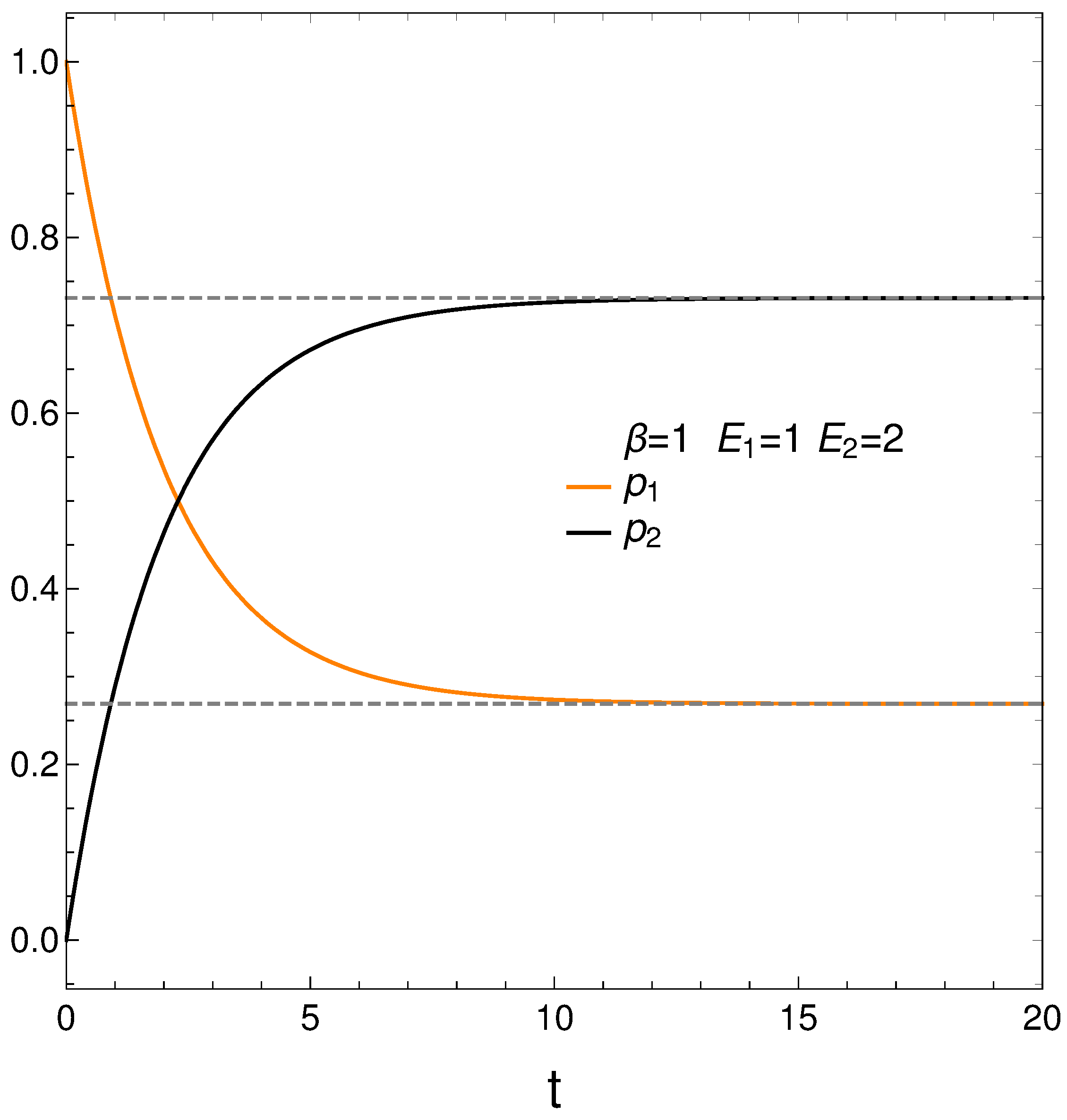
In analyzing our master equation, time is always measured in arbitrary units. We start by looking at the time evolution of our two probabilities in Figure 1. We see that they eventually cross each other, which anticipates an interesting situation.

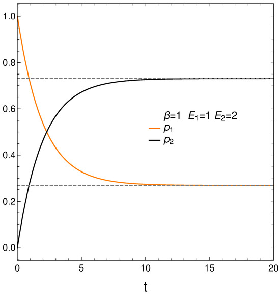
Figure 1. $p_1$ and $p_2$ vs. t (arbitrary units), with $E_1=1$, $E_2=2$, $\beta =1$, and initial conditions $p_1\left(0\right)=1-p_2\left(0\right)=0$.

We begin with $p_1$ and $p_2$. Figure 1 depicts the behavior of our two probabilities for the initial conditions $p_1\left(0\right)=1$ and $p_2\left(0\right)=0$ versus time in arbitrary units. They cross at a time $t_c\sim 2$. Here we have, in determining the constants $a_1$ and $a_2$ of Equation (3), $E_1=1$, $E_2=2$, $\beta =1$, and $T={\displaystyle \frac{1}{\beta }}$. This T-value is also used in computing the free energy F. Note that stationarity is eventually reached.

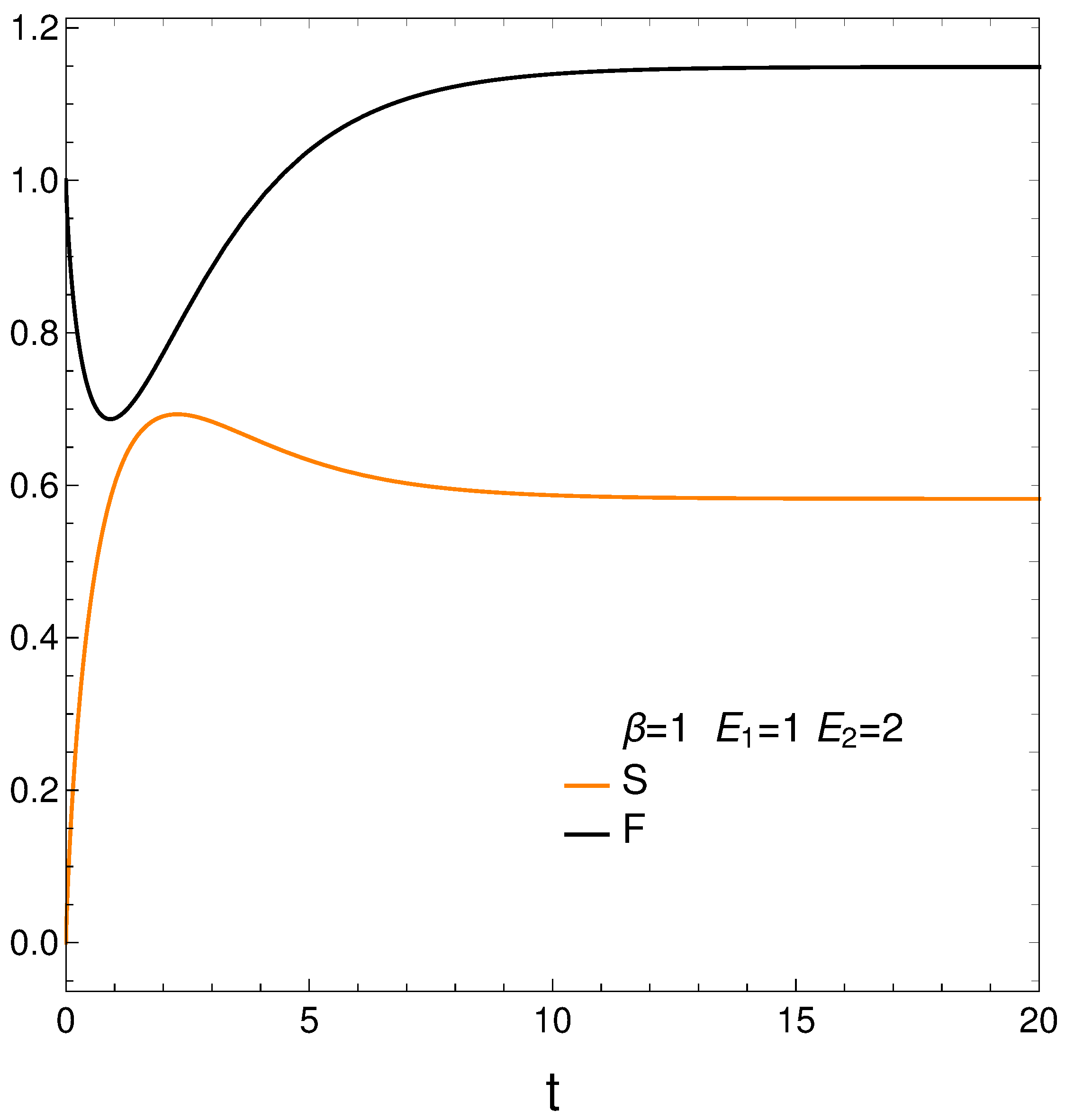
We compute next the entropy S, Helmholtz free energy F, and mean energy U from their definitions and then plot the first two of them in Figure 2. We have [12]

$$\begin{array}{ccc}\hfill S& =& -p_{1}ln{p}_1-p_{2}ln{p}_2\hfill \end{array}$$

(13)

$$\begin{array}{ccc}\hfill F& =& U-TS\hfill \end{array}$$

(14)

$$\begin{array}{ccc}\hfill U& =& E_1{p}_1+E_2{p}_2\hfill \end{array}$$

(15)

Remember that the lower the free energy of a system, the more stable it tends to be since spontaneous changes involve a decrease in F. Results are given in Figure 2. Notice that the system reaches a minimum value for F (color black, maximum stability) at a certain time $t_M\sim 1$. However, the master equation mechanism takes the system away from the minimum till it reaches stationarity. We discover that our master equation mechanism prefers stationarity over stability. Not surprisingly, the system reaches maximum entropy S (color orange, disorder) at a time close to $t_c\sim 2$ (see above).

It seems that our master equation describes a process of the initial growth of the entropy and the useful available energy followed by one of equilibration at higher values of both S and F.

Figure 2. S (orange) and F (black) vs. time t, with $E_1=1$, $E_2=2$, $\beta =1$, $p_1\left(0\right)=1$, and $p_2\left(0\right)=0$. Notice that the system reaches a minimum value for F (maximum stability) at a time $t_M$. However, the master equation mechanism takes the system away from the minimum till it reaches stationarity. We discover that our master equation mechanism prefers stationarity over stability. Not surprisingly, the system reaches maximum entropy (disorder) almost at the time $t_c$.

Figure 2. S (orange) and F (black) vs. time t, with $E_1=1$, $E_2=2$, $\beta =1$, $p_1\left(0\right)=1$, and $p_2\left(0\right)=0$. Notice that the system reaches a minimum value for F (maximum stability) at a time $t_M$. However, the master equation mechanism takes the system away from the minimum till it reaches stationarity. We discover that our master equation mechanism prefers stationarity over stability. Not surprisingly, the system reaches maximum entropy (disorder) almost at the time $t_c$.

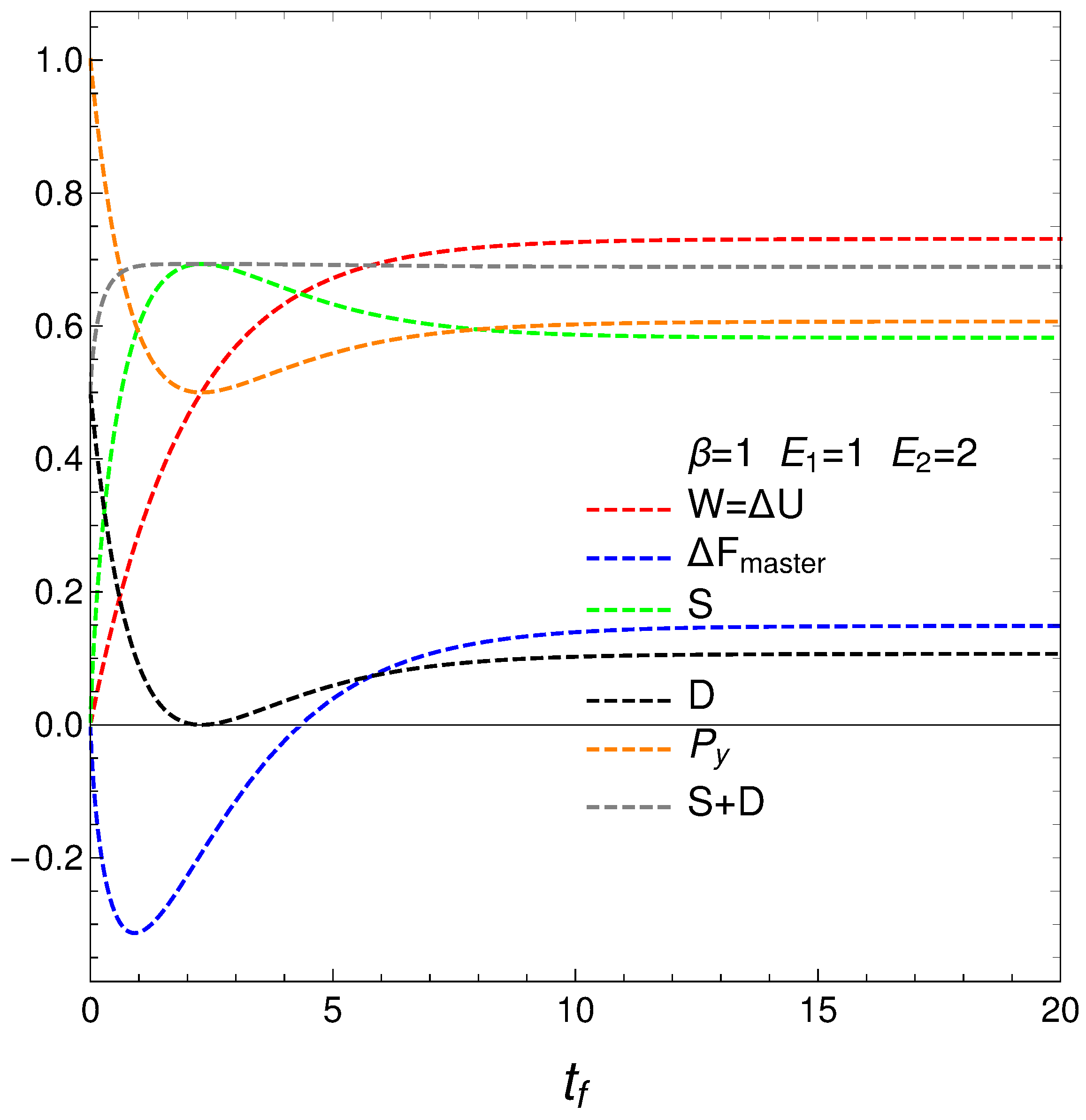
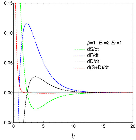
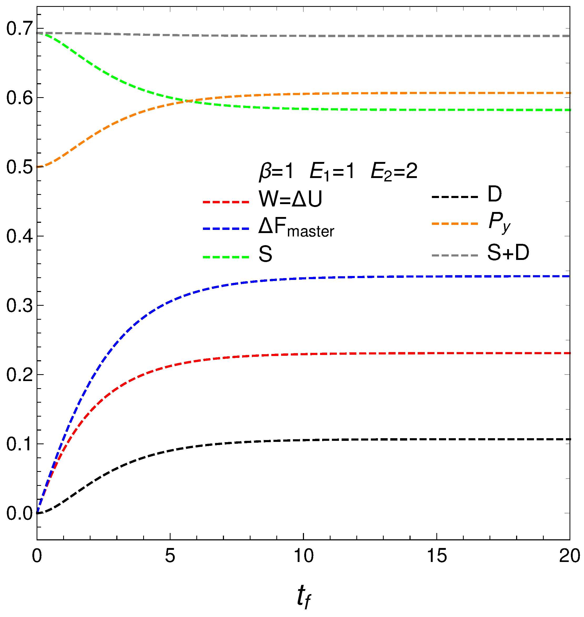
The following graph, Figure 3, depicts

• The mean energy difference $W=U\left(t\right)-U(t=0)$,
• The difference of the free energy $\Delta F_{master}=F_{master}\left(t\right)-F_{master}(t=0)$,
• The disequilibrium $D={(p_1-1/2)}^2+{(p_2-1/2)}^2$,
• The purity (degree of mixing in the quantum sense) $P_y=p_1^2+p_2^2$ where $0\le P_y\le 1$, with $P_y=1$ for a pure state,
• The entropy S, and
• The sum $S+D$.

nOTE that $S+D$ is almost constant as we approach the stationary zone, which reinforces our assertions above about D representing order. Thus, we note that the sum of order plus disorder indicators approaches a constant value as we near stationarity.

The entropic and free energy behaviors are those displayed in Figure 2 above. The disequilibrium (order indicator) attains its minimum when S gets maximal, as expected. The purity starts being maximal at $t=0$, descends first afterwards, and then slightly increases till it reaches stationarity. Thus, our master equation transforms a pure state into a stationary mixed one. The master equation is able to yield useful free energy only for a very short time in which it creates disorder.

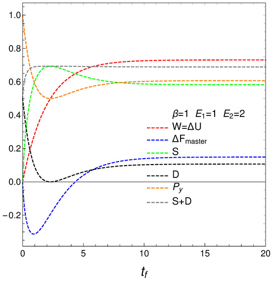
Figure 3. This graph is intended as a complement of Figure 2. The horizontal axis displays the final time $t_f$. The plot depicts the mean energy difference $W=\Delta U=U(t_f-U(t=0)$. In similar fashion, also $\Delta F$, the disequilibrium D, purity $P_y$, and entropy S versus $t\equiv t_f$, with $E_1=1$, $E_2=2$, $\beta =1$, and initial conditions $p_1\left(0\right)=1$ and $p_2\left(0\right)=0$. What we learned from Figure 2 is reinforced here using different quantities. Note that near stationarity order again balances disorder.

Figure 3. This graph is intended as a complement of Figure 2. The horizontal axis displays the final time $t_f$. The plot depicts the mean energy difference $W=\Delta U=U(t_f-U(t=0)$. In similar fashion, also $\Delta F$, the disequilibrium D, purity $P_y$, and entropy S versus $t\equiv t_f$, with $E_1=1$, $E_2=2$, $\beta =1$, and initial conditions $p_1\left(0\right)=1$ and $p_2\left(0\right)=0$. What we learned from Figure 2 is reinforced here using different quantities. Note that near stationarity order again balances disorder.

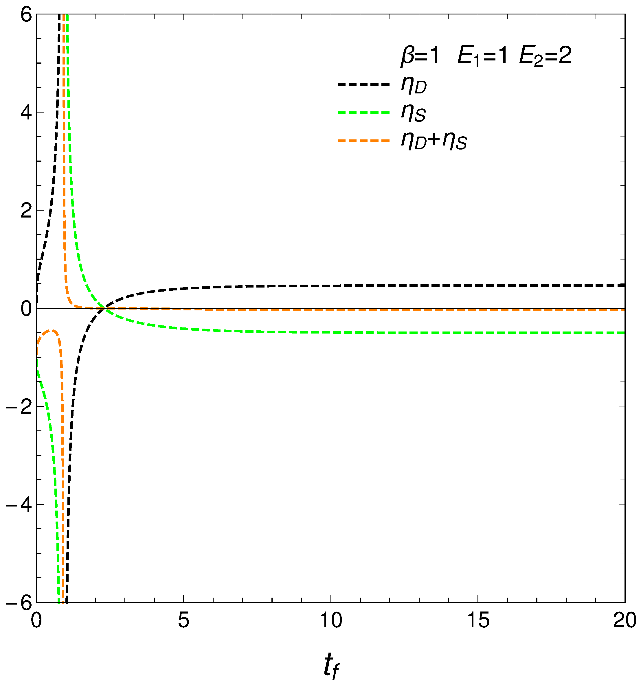
We move now to the plot in Figure 4, versus final time $t_f$, the energetic-cost indicators $dS/dt$, $dF/dt$, $dD/dt$.

Figure 4. $dS/dt$, $dF/dt$, $dD/dt$, and $d(S+D)/dt$ vs. $t\equiv t_f$. One sets $E_1=1$, $E_2=2$, $\beta =1$, and initial conditions (IC) $p_1\left(0\right)=1$−$p_2\left(0\right)=0$. This graph is still another complement to Figure 2, using different quantities from those of Figure 2 and Figure 3. Maxima and minima are found at the right of $t_M$ and are also <5. Their message is thus reinforced here.

5. Regime Transitions

We reach interesting insights at this stage. Consider now the approximate energetic-cost indicators

$$\begin{array}{ccc}\hfill {\eta }_D& =& {\displaystyle \frac{dD/dt}{dF/dt}}\hfill \end{array}$$

(16)

$$\begin{array}{ccc}\hfill {\eta }_S& =& {\displaystyle \frac{dS/dt}{dF/dt}},\hfill \end{array}$$

(17)

that determine how much free energy is expended or received so as to change either the disequilibrium or the entropy. We call them approximate because, strictly speaking, T and, as a consequence, F are strictly determined only at the final evolution-stage of stationarity, where there is equilibrium with the heat reservoir. Anyway, our $\eta$’s behavior is rather surprising, as can be seen in Figure 5. The free energies required to effect our changes diverge at the time at which $p_1=p_2$ where the entropy is a maximum, which we called $t_M$. The divergence at this time indicates a temporary singularity.

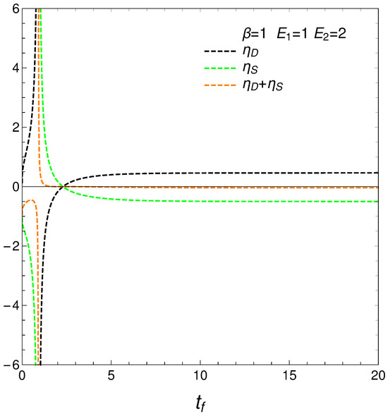
Figure 5. ${\eta }_D$ and ${\eta }_S$ vs. $t\equiv t_f$. One sets $E_1=1$, $E_2=2$, $\beta =1$, and IC $p_1\left(0\right)=1$ y $p_2\left(0\right)=0$. Also, the $\eta$ value corresponding to $S+D$ is shown. The three quantities diverge (regime-transition) at the time for which $p_1=p_2$. Our very simple system exhibits divergence there.

Finding a temporary singularity in our master equation is a noteworthy observation that can have several implications and interpretations. The temporary singularity suggests a critical point in the dynamical behavior of the system where conventional descriptions may break down.

As our study shows divergence in the approximate energetic costs ${\eta }_S$ and ${\eta }_D$ as the system approaches uniformity, the singularity may represent a turning point in the system’s behavior. This critical transition could signify a shift from one regime of behavior to another, highlighting the complexity of transitions between ordered and disordered states.

The singularity might indicate that the system temporarily loses its physical meaning at that point, emphasizing the idea that equilibrium is a dynamic state, not a static one. This indicates that the system does not simply settle into equilibrium but rather navigates through complex paths that reflect changes in entropy and free energy.

5.1. Two Regimes for Our Master Equation

One can describe the behavior of the master equation as representing two distinct regimes, with a temporary loss of physical sense at the divergence time $t_M$. That is, the master equation shows different behaviors before and after a critical divergence time, $t_M$. Initially, the system evolves according to the master equation, but as it approaches a uniform distribution ($p_1=p_2=1/2$), certain ratios (${\eta }_S$ and ${\eta }_D$) diverge. This divergence indicates a point where the current form of the master equation temporarily loses its physical meaning. Pre-Divergence: From the initial state up to $t_M$, the system evolves according to the master equation, with well-defined changes in entropy, distance, and free energy. The master equation provides a physically meaningful description of the system’s dynamics, which is governed by a linear interaction, and the ratios ${\eta }_S$ and ${\eta }_D$ behave regularly. Post-Divergence: from $t_M$ onward, the system settles into a new, well-behaved regime where the solutions of the master equation stabilize at finite values. This represents a new equilibrium or steady state. The dynamics are again well-described by the master equation, and the physical quantities stabilize, indicating a return to physical sense.

At time $t_M$ we face a temporary loss of physical meaning: the ratios ${\eta }_S$ and ${\eta }_D$ diverge, suggesting a temporary breakdown in the physical interpretation provided by the master equation. This time marks a critical transition in the system’s behavior, potentially indicating complex dynamics such as critical slowing down or a phase transition.

Summing up, the master equation describes two distinct regimes in the system’s dynamics. In the first regime, from the initial state up to a critical divergence time $t_M$, the system evolves predictably and the master equation retains physical meaning. At $t_f$, the system experiences a temporary divergence in key ratios, indicating a loss of physical sense. However, beyond this point, the system settles into a new, well-behaved regime where the master equation’s solutions stabilize at finite values, representing a new equilibrium or steady state. Thus, the master equation temporarily loses physical meaning only at the divergence time $t_M$ but remains valid in describing both pre- and post-divergence regimes. This framing highlights the temporary nature of the breakdown at $t_M$ and acknowledges the master equation’s validity in describing the system’s dynamics in both regimes.

5.2. Statistical Complexity

• Near equilibrium, small changes in one quantity (like free energy) can lead to disproportionately large changes in others (like entropy and distance in probability space).
• The divergence of these ratios is related to a phenomenon known as critical slowing down, where the rate of change of a system’s state variables becomes very slow near equilibrium (or near a critical point in phase transitions). As the free energy change rate $dF/dt$ approaches zero, the system’s response to external perturbations also slows down, indicating that the system is in a state of heightened sensitivity and complexity.
• The ratios involve the rates of change of entropy, distance, and free energy, showing that these variables are interdependent. This interdependence means that changes in one variable can have complex effects on the others. Such interdependence and feedback loops are characteristic of complex systems, where the behavior of the whole system cannot be easily inferred from the behavior of individual parts.
• As the system approaches the uniform distribution, small differences in initial conditions can lead to significantly different trajectories in the state space. This sensitivity is another hallmark of complexity, often observed in chaotic systems.
• The divergence to the plus–minus infinity of the ratios suggests emergent behavior, where the macroscopic properties (like the ratios ${\eta }_S$ and ${\eta }_D$) exhibit behaviors that are not straightforwardly predictable from the microscopic rules (the master equation governing the probabilities $p_1$ and $p_2$). Emergence is a key feature of complex systems.
• The described behavior indicates a high level of complexity in the system’s approach to equilibrium. This complexity arises from the dynamics’ critical slowing down, the interdependence of state variables, the sensitivity to initial conditions, and the ensuing emergent behavior, all of which are characteristic of complex systems in statistical mechanics.

Our master equation displays a picturesque regime’s transition in our novel quantities when the entropy attains a maximum.

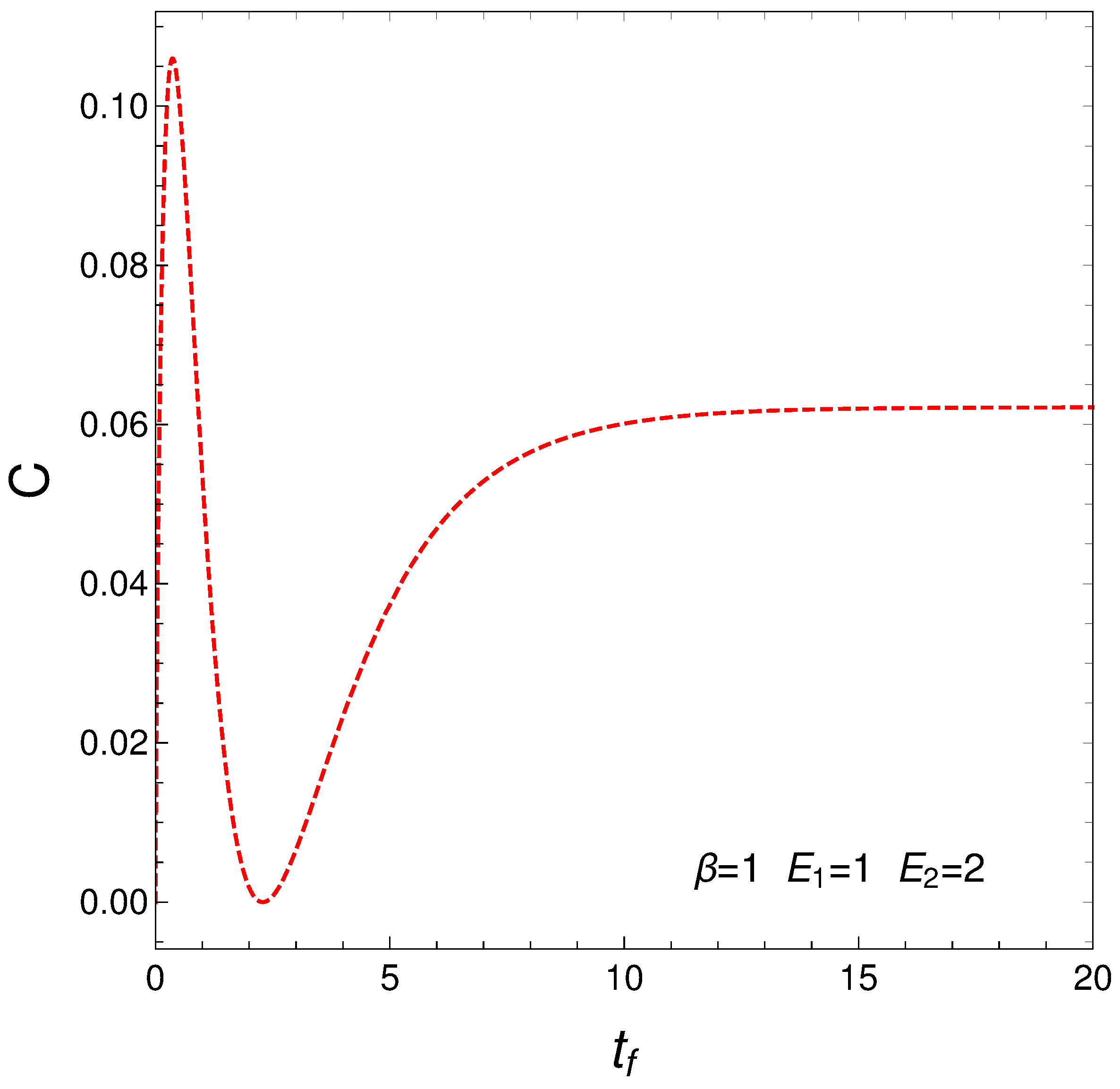
5.3. The Lopez–Ruiz, Mancini, and Calvet Form for the Statistical Complexity C

This measure of the statistical complexity $C=SD$ originated about 25 years ago and has become quite popular, being used for variegated purposes. We just cite here [3,4,5,6,7]. We now depict in Figure 6 C versus time in the context of our master equation. We clearly see that our two regimes exhibit different levels of complexity.

Figure 6. Statistical complexity evolution with time. Two different regimes emerge. As before, one sets $E_1=1$, $E_2=2$, $\beta =1$, and IC $p_1\left(0\right)=1$ y $p_2\left(0\right)=0$.

6. Initial Conditions ${\mathit{p}}_{\mathbf{1}}={\mathit{p}}_{\mathbf{2}}=\mathbf{1}/\mathbf{2}$ of Maximum Entropy

Given its great importance, consider, in more detail, the solutions of our master equation for $p_1=p_2=1/2$ at $t=0$. The results for these maximum entropy initial conditions (MSIC) are plotted below. The entropy, of course, descends, and the remaining quantifiers increase till reaching stationarity. See Figure 7 below.

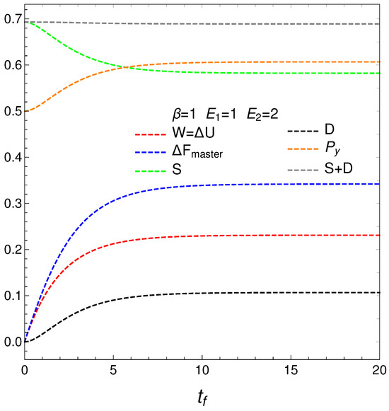
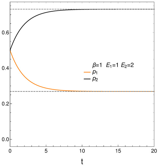
Figure 7. MSIC. Thermal quantities versus time. One sets $\beta =1$, $E_1=1$, and $E_2=2$. The entropy diminishes. The remaining quaifiers increase. Stationarity is reached.

7. The Order($\mathit{D}$)–Disorder($\mathit{S}$) Equation Generated by the Master Equation

From its definition $D={(p_1-1/2)}^2+{(p_2-1/2)}^2$ and from the relation $p_1+p_2=1$, we gather that $p_1={\displaystyle \frac{1}{2}}\mp \sqrt{D/2}$ and $p_2=1-p_1={\displaystyle \frac{1}{2}}\pm \sqrt{D/2}$, with

$$0<D<1/2.$$

(18)

From the entropic definition, one then finds S vs D, which turns out to be, for any values of $\beta$, $E_1$, and $E_2$, the rather beautiful expression that gives the entropy solely in terms of the order quantifier for any two-level system:

$$\begin{array}{cc}\hfill S=& -\left({\displaystyle \frac{1}{2}}+\sqrt{{\displaystyle \frac{D}{2}}}\right)ln\left({\displaystyle \frac{1}{2}}+\sqrt{{\displaystyle \frac{D}{2}}}\right)-\hfill \\ \hfill & -\left({\displaystyle \frac{1}{2}}-\sqrt{{\displaystyle \frac{D}{2}}}\right)ln\left({\displaystyle \frac{1}{2}}-\sqrt{{\displaystyle \frac{D}{2}}}\right)\hfill \end{array}$$

(19)

The above relation is independent of $E_i$ and of $\beta$. We plot in Figure 8 $S\left(t\right)$ versus $D\left(t\right)$ with time as the parameter. The solid curve represents the above equation $S\left(D\right)$. Of course, if the order is maximal the entropy vanishes. The circles represent specific parameters’ values of the energies in the following fashion:

• Orange: $p_1\left(0\right)=1,p_2\left(0\right)=0,\beta =1,E_1=1E_2=10$;
• Blue: $p_1\left(0\right)=1,p_2\left(0\right)=0,\beta =1,E_1=1E_2=2$;
• Green: $p_1\left(0\right)=1,p_2\left(0\right)=0,\beta =1,E_1=2E_2=1$;
• Red: $p_1\left(0\right)=1,p_2\left(0\right)=0,\beta =1,E_1=4E_2=1$.

It is clear from Figure 8 that S decreases as D grows. But this happens neither linearly nor in complex manner.

The ability to express entropy S, for any two-level system, solely in terms of a simple function of the order indicator D is a significant and intriguing result with several important implications. Here are some points regarding this finding:

1.- Direct Relationship Between Order and Disorder: By demonstrating that entropy can be quantified through the order indicator D, we establish a clear and direct mathematical relationship between the concepts of order and disorder. This reinforces the idea that entropy, often seen as a measure of disorder, can indeed be understood through a lens that focuses on the structure and arrangement of a system.

2.- Simplicity and Elegance: The simplicity of the resulting function highlights the elegance of the underlying dynamics captured by the master equation. A straightforward relationship between two fundamental concepts indicates a well-structured system where complex behaviors may arise from relatively simple rules.

3.- Educational Value: This finding can serve as a powerful pedagogical tool in physics education. Illustrating how a complex quantity like entropy can be directly derived from a more intuitive measure of order (like D) can help students grasp abstract concepts more effectively. It can spark discussions about the connections between various thermodynamic parameters and enhance one’s understanding of the principles of statistical mechanics.

4.- Implications for Statistical Mechanics: The ability to express S in terms of D opens up new avenues for research within statistical mechanics. It suggests that studying the order within a system may provide insights into its configuration and transition behaviors. This understanding could be beneficial in fields ranging from materials science to biological systems, where order–disorder transitions are pivotal.

5.- Potential for Applications: By relating entropy to the order indicator, one may discover new applications for the order measure D. For instance, the function expressing S in terms of D could inform predictions about system behavior under different conditions, aiding in the control and optimization of processes in various scientific and engineering applications.

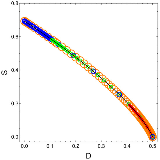
Figure 8. S vs. D for variegated selection of the parameters $E_1,E_2$ that is detailed in the text. Also, $\beta =1$ and $p_1\left(0\right)=1,p_2\left(0\right)=0$. Black line underling represents Equation (19).

Figure 8. S vs. D for variegated selection of the parameters $E_1,E_2$ that is detailed in the text. Also, $\beta =1$ and $p_1\left(0\right)=1,p_2\left(0\right)=0$. Black line underling represents Equation (19).

Polynomial Approximations for the Relation S Versus D

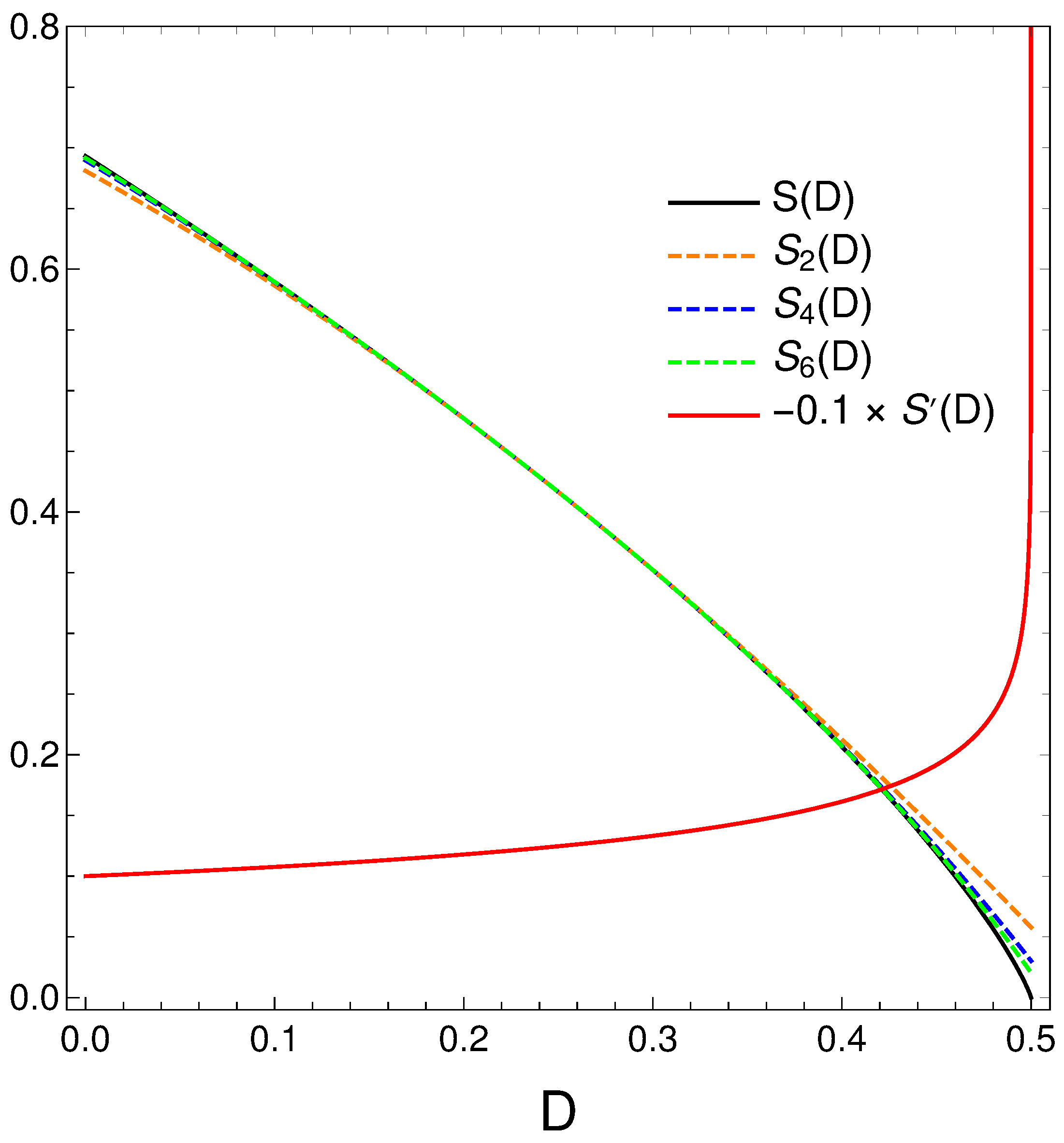
We now take a closer look at the order–disorder relation that our master equation displays. We thus proceed to make a Taylor expansion of $S\left(D\right)$ around $D=1/4$ and obtain

$$\begin{array}{cc}\hfill S\left(D\right)\approx & {\displaystyle \frac{3}{2}}ln\left[2\right]+{\displaystyle \frac{\sqrt{2}}{4}}ln[3-2\sqrt{2}]-{\displaystyle \frac{\sqrt{2}ln[3-2\sqrt{2}]}{{(2+\sqrt{2})}^2(-3+2\sqrt{2})}}(D-{\displaystyle \frac{1}{4}})-\hfill \\ \hfill & -{\displaystyle \frac{8+2\sqrt{2}ln[3-2\sqrt{2}]}{{(2+\sqrt{2})}^4{(-3+2\sqrt{2})}^2}}{(D-{\displaystyle \frac{1}{4}})}^2-{\displaystyle \frac{32+24\sqrt{2}ln[3-2\sqrt{2}]}{3{(2+\sqrt{2})}^6{(-3+2\sqrt{2})}^3}}{(D-{\displaystyle \frac{1}{4}})}^3-\hfill \\ \hfill & -{\displaystyle \frac{466+120\sqrt{2}ln[3-2\sqrt{2}]}{3{(2+\sqrt{2})}^8{(-3+2\sqrt{2})}^4}}{(D-{\displaystyle \frac{1}{4}})}^4-{\displaystyle \frac{5504+3360\sqrt{2}ln[3-2\sqrt{2}]}{15{(2+\sqrt{2})}^{1}0{(-3+2\sqrt{2})}^5}}{(D-{\displaystyle \frac{1}{4}})}^5-\hfill \\ \hfill & -{\displaystyle \frac{65792+20160\sqrt{2}ln[3-2\sqrt{2}]}{15{(2+\sqrt{2})}^{1}2{(-3+2\sqrt{2})}^6}}{(D-{\displaystyle \frac{1}{4}})}^6+O\left(D^7\right)\hfill \end{array}$$

(20)

We plot below in Figure 8 $S\left(D\right)$ (black) and minus its derivative ${\displaystyle \frac{dS\left(D\right)}{dD}}$ (red) [in fact, $-0.1\times {\displaystyle \frac{dS\left(D\right)}{dD}}$)]. Orange, blue, and green dashed curves represent, respectively, approximations to $S\left(D\right)$ of degree two, four, and six. Note that the relation disorder versus order looks quasi linear in some regions but is not quite. When the order-degree gets near its maximum value of one half, the disorder diminishes in a quite rapid fashion, as the derivative plot illustrates. Summing up, the order–disorder relation for our master equation displays some quirky traits.

We plot next in Figure 9 some approimations to the relation $S-D$.

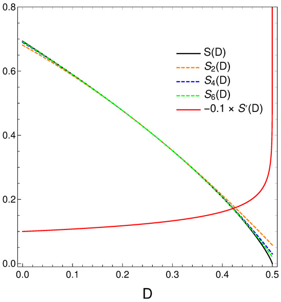
Figure 9. Polynomial approximations to the relation $S-D$ of orders two, four, and six in different colors. The exact $S\left(D\right)$ is given in black. We also depict $-0.1\times {\displaystyle \frac{dS\left(D\right)}{dD}}$ in orange.

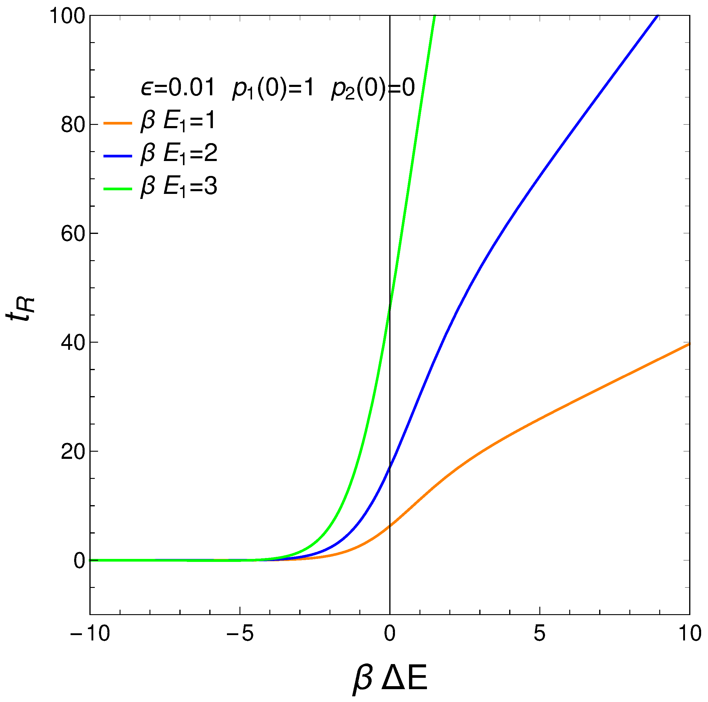
8. Relaxation Time t_R

We define our system’s relaxation $t_R$ as the time-interval needed to reach stationarity so that $p_i\left(t\right)$ no longer display significant changes. We can require, for instance, that $|p_i\left(t_R\right)-p_i^{st}|<ϵp_i^{st}$, with $ϵ=1/100$. Thus, from Equations (3) and (4), we gather that

$$\begin{array}{ccc}\hfill t_R& =& {\displaystyle \frac{{\mathrm{e}}^{\beta E_1}}{1+{\mathrm{e}}^{-\beta \Delta E}}}\left\{\beta \Delta E+ln\left|p_1\left(0\right)-{\mathrm{e}}^{-\beta \Delta E}{p}_2\left(0\right)\right|-ln\left[ϵ\right]\right\},\hfill \end{array}$$

(21)

where $\Delta E=E_2-E_1$. The relation is displayed next for different values of the pre-factor $\beta E_1$. The initial conditions are $p_1\left(0\right)=1$ $p_2\left(0\right)=0$. For a considerable range of $\beta E_1$, the relaxation time is independent of this quantity. See the results plotted in Figure 10.

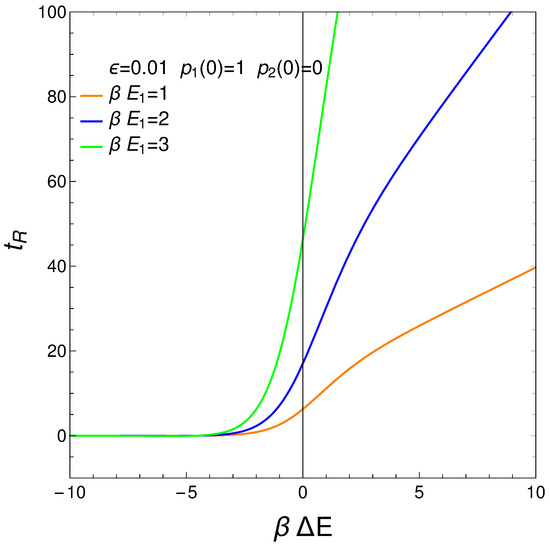
Figure 10. $t_R$ vs. $\beta \Delta E$ for $\beta E_1=1,2,3$. $ϵ$ is the approximation’s degree (see text). Save for very small (negative) values of $g=\beta E_1$, the relaxation time is constant. If g becomes small, $t_R$ augments. This fact is of interest for high temperatures, of course. It makes sense that for such temperatures it should become more difficult to reach equilibration. Positive values of $\beta E_1$ make little sense in the context of our master equation.

9. Relating the Derivatives $\mathit{dS}/\mathit{dt}$ and $\mathit{dD}/\mathit{dt}$

From our formalism, we immediately obtain the important relation

$${\displaystyle \frac{dS}{dt}}={\displaystyle \frac{\sqrt{2}}{4\sqrt{D}}}ln\left[{\displaystyle \frac{1-\sqrt{2D}}{1+\sqrt{2D}}}\right]{\displaystyle \frac{dD}{dt}}.$$

(22)

This relation between the rates of change of order and disorder is illustrated next. These rates are positively correlated, as one intuitively expects. We consider two situations: (a) $E_2>E_1$, and (b) $E_1>E_2$. No important differences ensue between (a) and (b). See the results depicted in Figure 11.

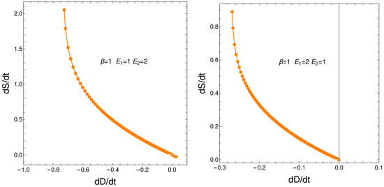
Figure 11. $dS/dt$ versus $dD/dt$ for $\beta =1$ and $p_1\left(0\right)=1-p_2\left(0\right)=0$. Left: $E_1=1$ and $E_2=2$. Right: $E_1=2$ and $E_2=1$.

10. Conclusions

We have studied, in detail, a very simple master equation that displays a complex physics, as the divergences depicted in Figure 5 illustrate. Our present master equation hides a powerful mechanism that is able to produce two different regimes with a quite sharp transition between them, signaled by a specific quantifier. The transition is associated with a regime-change, implying a considerable energetic cost. This master equation’s simplicity allows for easy access to recondite facts of the pertinent process.

Our master equation describes a process of initial growth of both the entropy and the useful available energy followed by one of equilibration at higher values of both S and F. Note that near the stationary stage order balances disorder.

We represent the notion of order by the disequilibrium D and (of course) disorder by the entropy S. Surprisingly enough, we find that their sum tends to be a constant for much of the time under a variety of conditions because the meaning of S was established more than a century ago or results give new validity to the newer notion of disequilibrium. Note that Figure 8 shows that the degree of disorder greatly accelerates itself as D tends towards its maximum possible value. For smaller D values, the rate of S growth is rather uniform.

Simple exactly solvable models are often used as starting points for understanding more complex systems. Our discovery of regime-transitions (RT) here can serve as a model system to investigate the nature of RT and their scaling behavior. This knowledge might be applied to more intricate systems in the future. Discovering phase transitions in an elementary exactly solvable master equation can also have methodological importance. It demonstrates that our analytical and modeling techniques are capable of capturing non-trivial collective behaviors and can be applied to other systems.

The existence of two regimes in the master equation is a sign of complexity due to the following reasons:

• Often in complex systems, small changes in initial conditions or parameters can lead to vastly different outcomes.
• The divergence at the critical transition point is indicative of phenomena such as critical slowing down, where the system’s response to perturbations becomes significantly slower near equilibrium. Such critical points are often associated with phase transitions in complex systems.
• In complex systems, variables are often interdependent in non-trivial ways. The fact that the ratios ${\eta }_S={\displaystyle \frac{dS/dt}{dF/dt}}$ and ${\eta }_D={\displaystyle \frac{dD/dt}{dF/dt}}$ diverge suggests intricate inter-dependencies between entropy, distance, and free energy, contributing to the system’s overall complexity.
• The existence of multiple regimes with distinct stable states (pre- and post-divergence) suggests that the system can settle into different configurations depending on its initial conditions and evolution. This multiplicity of stable states is a characteristic feature of complex systems.
• The transition between regimes highlights the system’s sensitivity to initial conditions. Complex systems often exhibit such sensitivity, where initial conditions or slight perturbations can lead to entirely different behaviors and outcomes.
• The stabilization into a new regime after the divergence indicates emergent behavior, where the system self-organizes into a new equilibrium or steady state. Emergent behavior is a key aspect of complexity, where the whole is more than the sum of its parts.
• Summing up, the existence of two regimes in the master equation is a sign of complexity because it reflects critical transitions, interdependencies between variables, multiple stable states, sensitivity to initial conditions, and emergent behavior. These factors collectively contribute to the intricate and often unpredictable nature of complex systems.

References

- López-Ruiz, R.; Mancini, H.; Calbet, X. A statistical measure of complexity. Phys. Lett. A 1995, 209, 321–326. [Google Scholar] [CrossRef]
- López-Ruiz, R. Complexity in some physical systems. Int. J. Bifurc. Chaos 2001, 11, 2669–2673. [Google Scholar] [CrossRef]
- Martin, M.T.; Plastino, A.; Rosso, O.A. Statistical complexity and disequilibrium. Phys. Lett. A 2003, 311, 126–132. [Google Scholar] [CrossRef]
- Rudnicki, L.; Toranzo, I.V.; Sánchez-Moreno, P.; Dehesa, J.S. Monotone measures of statistical complexity. Phys. Lett. A 2016, 380, 377–380. [Google Scholar] [CrossRef]
- López-Ruiz, R. A Statistical Measure of Complexity in Concepts and Recent Advances in Generalized Infpormation Measures and Statistics; Kowalski, A., Rossignoli, R., Curado, E.M.C., Eds.; Bentham Science Books: New York, NY, USA, 2013; pp. 147–168. [Google Scholar]
- Sen, K.D. (Ed.) Statistical Complexity, Applications in Elctronic Structure; Springer: Berlin/Heidelberg, Germany, 2011. [Google Scholar]
- Martin, M.T.; Plastino, A.; Rosso, O.A. Generalized statistical complexity measures: Geometrical and analytical properties. Phys. A 2006, 369, 439–462. [Google Scholar] [CrossRef]
- Anteneodo, C.; Plastino, A.R. Some features of the López-Ruiz-Mancini-Calbet (LMC) statistical measure of complexity. Phys. Lett. A 1996, 223, 348–354. [Google Scholar] [CrossRef]
- Yong, S.; Yu, C. Operational resource theory of total quantum coherence. Ann. Phys. 2018, 388, 305. [Google Scholar] [CrossRef]
- Takada, A.; Conradt, R.; Richet, P. Residual entropy and structural disorder in glass: A two-level model and a review of spatial and ensemble vs. temporal sampling. J. Non-Cryst. Solids 2013, 360, 13–20. [Google Scholar] [CrossRef]
- Plastino, A.; Ferri, G.; Plastino, A. Heating, Cooling, and Equilibration of an Interacting Many-Fermion System. J. Mod. Phys. 2020, 11, 1312–1325. [Google Scholar] [CrossRef]
- Pathria, R.K. Statistical Mechanics, 2nd ed.; Butterworth-Heinemann: Oxford, UK, 1996. [Google Scholar]
Disclaimer/Publisher’s Note: The statements, opinions and data contained in all publications are solely those of the individual author(s) and contributor(s) and not of MDPI and/or the editor(s). MDPI and/or the editor(s) disclaim responsibility for any injury to people or property resulting from any ideas, methods, instructions or products referred to in the content. |
© 2025 by the authors. Licensee MDPI, Basel, Switzerland. This article is an open access article distributed under the terms and conditions of the Creative Commons Attribution (CC BY) license (https://creativecommons.org/licenses/by/4.0/).