Abstract
This paper investigates the use of deep learning techniques in order to perform energy demand forecasting. To this end, the authors propose a mixed architecture consisting of a convolutional neural network (CNN) coupled with an artificial neural network (ANN), with the main objective of taking advantage of the virtues of both structures: the regression capabilities of the artificial neural network and the feature extraction capacities of the convolutional neural network. The proposed structure was trained and then used in a real setting to provide a French energy demand forecast using Action de Recherche Petite Echelle Grande Echelle (ARPEGE) forecasting weather data. The results show that this approach outperforms the reference Réseau de Transport d’Electricité (RTE, French transmission system operator) subscription-based service. Additionally, the proposed solution obtains the highest performance score when compared with other alternatives, including Autoregressive Integrated Moving Average (ARIMA) and traditional ANN models. This opens up the possibility of achieving high-accuracy forecasting using widely accessible deep learning techniques through open-source machine learning platforms.
1. Introduction
The forecasting of demand plays an essential role in the electric power industry. Thus, there are a wide variety of methods for electricity demand prediction ranging from those of the short term (minutes) to long term (weeks), while considering microscopic (individual consumer) to macroscopic (country-level) aggregation levels. This paper is focused on macroscopic power forecasting in the medium term (hours).
To date, researchers are in agreement that electrical demand arises from complex interactions between multiple personal, corporate, and socio-economic factors [1]. All these sources make power demand forecasting difficult. Indeed, an ideal model able to forecast the power demand with the highest possible level of accuracy would require access to virtually infinite data sources in order to feed such a model with all the relevant information. Unfortunately, both the unavailability of the data and the associated computational burden mean that researchers investigate approximate models supplied with partial input information.
Within this framework, the prediction of power consumption has been tackled from different perspectives using different forecasting methodologies. Indeed, there is a rich state of the art of methods which, according to the the authors of [1], can be divided into the following main categories:
- Statistical models: Purely empirical models where inputs and outputs are correlated using statistical inference methods, such as:
- ○
- Cointegration analysis and ARIMA;
- ○
- Log-linear regression models;
- ○
- Combined bootstrap aggregation (bagging) ARIMA and exponential smoothing.
Although some authors [2] report substantial improvements in the forecast accuracy of demand for energy end-use services in both developed and developing countries, the related models require the implementation of sophisticated statistical methods which are case-dependent with respect to their application. These facts hinder statistical models from forming an affordable and consistent basis for a general power demand forecasting approach.
- Grey models: These combine a partial theoretical structure with empirical data to complete the structure. When compared to purely statistical models, grey models require only a limited amount of data to infer the behavior of the electrical system. Therefore, grey models can deal with partially known information through generating, excavating, and extracting useful information from what is available. In return, the construction of the partial theoretical structure required by grey models is resource-demanding in terms of modeling. Thus, the cost of an accurate grey model for a particular application is usually high.
- Artificial intelligence models: Traditional machine learning models are data-driven techniques used to model complex relationships between inputs and outputs. Although the basis of machine learning is mostly statistical, the current availability of open platforms to easily design and train models contributes significantly to access to this technology. This fact, along with the high performance achieved by well-designed and trained machine learning models, provides an affordable and robust tool for power demand forecasting.
However, traditional machine learning models require a pre-processing step to perform the extraction of the main features of the input data; this generally involves the manual construction of such a module. To overcome this requirement (as depicted in Figure 1) modern deep learning techniques [3] have the capacity to integrate feature learning and model construction into just one model. According to this approach, the original input is transferred to more abstract representations in order to allow the subsequent model layers to find the inherent structures.
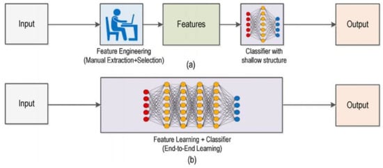
Figure 1.
Comparison between traditional machine learning models (a) requiring manual feature extraction, and modern deep learning structures (b) which can automate all the feature and training process in an end-to-end learning structure.
In this paper, the authors focus the analysis on predicting the energy demand based on artificial intelligence models. Nevertheless, although modern deep learning techniques have attracted the attention of many researchers in a myriad of areas, many publications related to power demand forecasting use traditional machine learning approaches such as artificial neural networks.
As commented above, the use of ANNs in the energy sector has been widely researched. Thanks to their good generalization ability, ANNs have received considerable attention in smart grid forecasting and management. A comparison between the different methods of energy prediction using ANN is proposed in [4] by classifying these algorithms into two groups.
On the one hand, the first group consists of traditional feedforward neural networks with only one output node to predict next-hour or next-day peak load, or with several output nodes to forecast hourly load [5].
On the other hand, other authors opt for radial basis function networks [6], self-organizing maps [7], and recurrent neural networks [8].
Lie et al. compared three forecasting techniques, i.e., fuzzy logic (FL), neural networks (NNs), and autoregressive (AR) processes. They concluded that FL and NNs are more accurate than AR models [9]. In 2020, Chen Li presented an ANN for a short-term load forecasting model in the smart urban grids of Victoria and New South Wales in Australia.
Bo et al. proposed a combined energy forecasting mechanism composed of the back propagation neural network, support vector machine, generalized regression neural network, and ARIMA [10]. Wen et al. explored a deep learning approach to identify active power fluctuations in real time based on long short-term memory (LSTM) [11].
However, traditional ANN solutions have limited performance when there is a lack of large training datasets, a significant number of inputs, or when solving computationally demanding problems [12], which is precisely the case discussed in this paper.
Thus, the authors of this paper found a promising topic related to the application of modern deep learning structures to the problem of power demand forecasting. More specifically, this paper describes the novel use of a particular deep neural network structure composed of a convolutional neural network (widely used in image classification) followed by an artificial neural network for the forecasting of power demand with a limited number of information sources available.
The network structure of a CNN was first proposed by Fukushima in 1988 [13]. The use of CNNs has several advantages over traditional ANNs, including being highly optimized for processing 2D and 3D images and being effective in the learning and extraction of 2D image features [14]. Specifically, this is a quite interesting application for the purposes of this paper, since the authors here aim to extract relevant features from the temperature grid of France (as further explained in Section 2.1.2).
The technique used to locate important regions and extract relevant features from images is referred to as visual saliency prediction. This is a challenging research topic, with a vast number of computer vision and image processing applications.
Wang et al. [15] introduced a novel saliency detection algorithm which sequentially exploited the local and global contexts. The local context was handled by a CNN model which assigned a local saliency value to each pixel given the input of local images patches, while the global context was handled by a feed-forward network.
In the field of energy prediction, some authors have studied the modeling of electricity consumption in Poland using nighttime light images and deep neural networks [16].
In [17], an architecture known as DeepEnergy was proposed to predict energy demands using CNNS. There are two main processes in DeepEnergy: feature extraction and forecasting. The feature extraction is performed by three convolutional layers and three poling layers while the forecasting phase is handled by a fully connected structure.
Based on the conclusions and outcomes achieved in previous literature, the authors here conceptualize their solution which, as described in the next sections, is an effective approach to dealing with the power demand time series forecasting problem with multiples input variables, complex nonlinear relationships, and missing data.
Furthermore, the proposed deep learning structure has been applied to the particular problem of French power demand in a real-setting approach. The next section comprehensively describes the materials and data sources used to this end, so other researchers can replicate and adapt the work of this paper to other power demand forecasting applications. As shown later, the performance of this approach is equal to (if not better than) that of the reference Réseau de Transport d’Electricité (RTE) French power demand forecast subscription-based service. Moreover, the proposed model performs better than existing approaches, as described in the Results section.
2. Materials and Methods
2.1. Data Analysis
2.1.1. Power Demand Data
For this paper, the historical data of French energy consumption were downloaded from the official RTE website [18], which provides data from 2012 to present. A first analysis of this data results is shown in Figure 2, which shows a clear seasonal pattern on the energy demand.
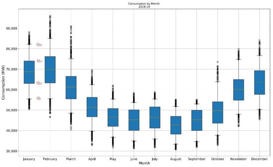
Figure 2.
Monthly French energy demand for the period 2018–2019. Qx indicates the X data percentiles. The colored lines within the Q25 and Q75 quartile boxes represent the median (orange line) and the mean (dashed green line). Points below and above Q25 and Q75 are shown as well.
The strong seasonal pattern in the energy demand is further backed by Figure 3, computed with the data of RTE, which depicts the correlation between energy consumption and temperature. As shown, an average variation of 1 °C during winter over the entire territory led to a variation of around 2500 MW in the peak consumption (equivalent to the average winter consumption of about 2 million homes) [18]. In the summer, the temperature gradient related to air conditioning was approximately 400 MW per °C.
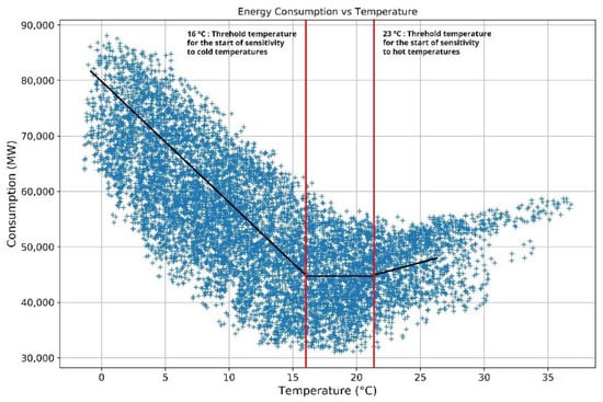
Figure 3.
Correlation between energy consumption and temperature as provided by the Réseau de Transport d’Electricité (RTE).
2.1.2. Weather Forecast Data
As explained in [19], the meteorological parameters are the most important independent variables and the main form of input information for the forecast of energy demand. Specifically, temperature plays a fundamental role in the energy demand prediction, since it has a significant and direct effect on energy consumption (please refer to Figure 3). Moreover, different weather parameters are correlated, so the inclusion of more than one may cause multicollinearity [19]. Accordingly, for this paper, temperature was the fundamental input used.
The weather forecast historical data were collected from Action de Recherche Petite Echelle Grande Echelle (ARPEGE), which is the main numerical weather prediction provider over the Europe–Atlantic domain.
As indicated in the ARPEGE documentation [20], the initial conditions of this model were based on four-dimensional variational assimilation (4D-Var) that incorporated very large and varied conventional observations (radio sounding, airplane measurements, ground stations, ships, buoys, etc.) as well as those from remote sensing (Advanced TIROS Operational Vertical Sounder (ATOVS), Special Sensor Microwave Imager Sounder (SSMI/S), Atmospheric Infrared Sounder (AIRS), Infrared Atmospheric Sounding Interferometer (IASI), Cross-Track Infrared Sounder (CRIS), Advanced Technology Microwave Sounder (ATMs), Spinning Enhanced Visible and Infrared Imager (SEVIRI), GPS sol, GPS satellite, etc.).
Although ARPEGE provided multiple forecast data related to weather (pressure, wind, temperature, humidity) with a full resolution of 0.1°, the authors of this paper found that the temperature data with a 1° resolution (as shown in Figure 4) were sufficient for the purpose of energy demand forecasting while maintaining easy-to-handle data sets. This finding is also aligned with the strong correlation of energy demand and temperature described in the preceding Section 2.1.1. Figure 4 shows the pre-processing results after reducing the granularity of the grid from 0.1° to 1°.
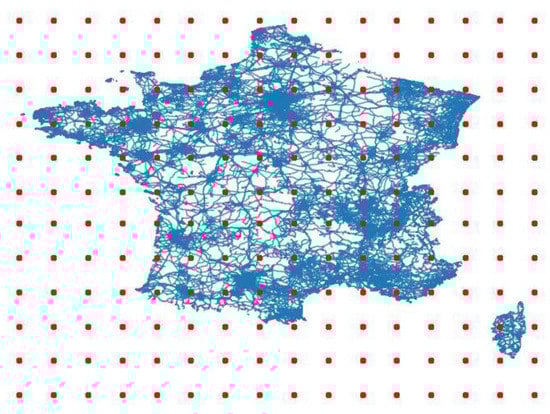
Figure 4.
Locations of temperature forecasting with a resolution of 1° over France.
A key issue related to weather forecasting was the availability of the data, since the providers released their predictions only at certain moments. In this case, the solution had to be be able to predict the French power demand for the day ahead (D+1) based on the weather forecasts at day D.
As depicted in Figure 5, the power demand forecast model was run at 08.00 every day (D), with the most recent weather forecast information available (released at 00.00), and provided a prediction of the energy demand during day D+1.
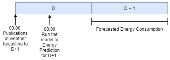
Figure 5.
Real setting of the energy demand forecasting problem. D: day.
2.2. Data Preparation
First, the historical datasets related to the French energy consumption (Section 2.1.1) and forecasted temperature (Section 2.1.2) were pre-processed to eliminate outliers, clean unwanted characters, and filter null data. Then, and as is usual practice when training machine learning models, the resulting data were divided into three datasets: training, validation, and testing.
Although the historical French consumption data provided by RTE date back to 2012, the authors of this paper had only access to the ARPEGE historical weather forecast data in the period spanning from 1 October 2018 to 30 September 2019. Although a wider availability of historical weather forecast data would have benefitted the generalization capability of the resulting machine learning model, the data set available still covered a whole year, so the seasonal influence was fully captured. Additionally, the authors randomly extracted eight full days from the original data set in order to further test the generalization performance of the model (as depicted in Figure 6 and further discussed in Section 3). This way, the remaining data sets were randomly divided as follows:
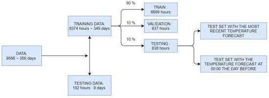
Figure 6.
Division of the original dataset (365 days) into testing and training data. The testing data were used as a complementary means to further analyze the generalization performance of the resulting model. The remaining training data were divided as usual: 80% train, 10% validation, and 10% testing.
- Training Dataset (80% of the data): The sample of data used to fit the model.
- Validation Dataset (10% of the data): The sample of data used to provide an unbiased evaluation of a model fit on the training dataset while tuning model hyperparameters.
- Test Dataset (10% of the data): The sample of data used to provide an unbiased evaluation of a final model fit on the training dataset.
2.3. Deep Learning Architecture
The deep learning architecture used in this paper (as shown in Figure 7) resembles those structures widely used in image classification: a convolutional neural network followed by an artificial neural network. The novelty of this paper is not the deep neural network itself but its application to the macroscopic forecast of energy demand. In fact, the aforementioned deep learning architecture was originally thought to automatically infer features from an input image (made of pixels) in order to subsequently classify such image in a certain category attending to the inferred specific features.
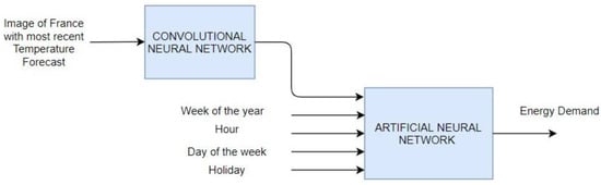
Figure 7.
Deep learning structure composed of a convolutional neural network followed by an artificial neural network adapted to the energy demand forecasting problem.
For the applications of this paper, the convolutional network received the temperature forecasts from multiple locations within the area of interest (in this case, France) instead of an image. Still, the convolutional network extracted a “feature” of such input, which may be understood as a representative temperature of France automatically calculated attending to the individual contribution of each location to the aggregated energy consumption. For instance, the temperature locations close to large consumption sites (such as highly populated areas) would be automatically assigned a larger weight when compared to other less populated areas.
As also discussed in Section 1, the advantage of the proposed deep learning structure with respect to traditional (and less sophisticated) machine learning structures is that this feature extraction is implicit to the model, and thus there is no need to design the feature extraction step manually.
As shown in Figure 7, the artificial neural network receiving the “featured” temperature from the convolutional network was also fed with additional information found to highly influence the energy demand as well, namely:
- Week of the year: a number from 1 to 52.
- Hour: a number from 0 to 23.
- Day of the week: a number from 0 to 6.
- Holiday: true (1) or false (0).
2.3.1. Convolutional Neural Network
As described by the authors in [21], convolutional neural networks, or CNNs, are a specialized kind of neural network for processing data, and have a known, grid-like topology. The name of “convolutional neural network” indicates that the network employs a mathematical operation called convolution, which is a specialized kind of linear operation. Traditional neural network layers use matrix multiplication to model the interaction between each input unit and each output unit. This means every output unit interacts with every input unit. Convolutional networks, however, typically have sparse interactions (also referred to as sparse connectivity or sparse weights). This characteristic provides the CNNs with a series of benefits, namely:
- They use a fewer number of parameters (weights) with respect to fully connected networks.
- They are designed to be invariant in object position and distortion of the scene when used to process images, which is a property shared when they are fed with other kinds of inputs as well.
- They can automatically learn and generalize features from the input domain.
Attending to these benefits, this paper used a CNN to extract a representative temperature of the area of interest (France) from the historical temperature forecast data as explained before. For the sake of providing an easy replication of the results by other researchers, the main features of the CNN designed for this paper were as follows:
- A two-dimensional convolutional layer. This layer created a convolution kernel that was convolved with the layer to produce a tensor of outputs. It was set with the following parameters:
- ○
- Filters: 8 integers, the dimensions of the output space.
- ○
- Kernel size: (2,2). A list of 2 integers specifying the height and width of the 2D convolution window.
- ○
- Strides: (1,1). A list of 2 integers specifying the stride of the convolution along with the height and width.
- ○
- Activation function: Rectified linear unit (ReLU)
- ○
- Padding: To pad input (if needed) so that input image was fully covered by the filter and was stride-specified.
- Average pooling 2D: Average pooling operation for special data. This was set with the following parameters:
- ○
- Pool size: (2,2). Factors by which to downscale.
- ○
- Strides: (1,1).
- Flattening: To flatten the input.
- A fully connected network providing the featured output temperature:
- ○
- Layer 1: 64 neurons, activation function: ReLU.
- ○
- Layer 2: 24 neurons, activation function: ReLU.
- ○
- Layer 3: 1 neuron, activation function: ReLU.
2.3.2. Artificial Neural Network.
As shown in Figure 7, the CNN output was connected to a fully connected multilayer artificial neural network (ANN) with the following structure.
- Layer 1: 256 neurons, activation function: ReLU.
- Layer 2: 128 neurons, activation function: ReLU.
- Layer 3: 64 neurons, activation function: ReLU.
- Layer 4: 32 neurons, activation function: ReLU.
- Layer 5: 16 neurons, activation function: ReLU.
- Layer 6: 1 neuron, activation function: ReLU.
The weights of all layers were initialized following a normal distribution with mean 0.1 and standard deviation 0.05.
2.3.3. Design of the Architecture
Different tests were performed in order to find the optimum number of layers and neurons. To this end, various networks structures were trained using the same data division for training, validation, and testing. Moreover, the training parameters were also optimized. To this effect, the different models were trained, repeatedly changing the learning parameters (as the learning rate) to find the optimal ones.
Once all the results were obtained, the objective was to find the model with the least bias error (error in the training set) as well as low validation and testing errors. Accordingly, model 5 of the table below was selected.
Finally, L2 regularization was added to our model in order to reduce the difference between the bias error and the validation/testing error. In addition, thanks to L2 regularization, the model was able to better generalize using data that had never been seen.
A summary of the tests performed can be seen in the Table 1 below:

Table 1.
Summary of the results of the different structures. ANN: artificial neural network; CNN: convolutional neural network.
2.4. Training
The training process of the proposed deep neural network was aimed at adjusting its internal parameters (resembling mathematical regression), so the structure was able to correlate its output (the French energy demand forecast) with respect to its inputs.
What separates deep learning from a traditional regression problem is the handling of the generalization error, also known as the validation error. Here, the generalization error is defined as the expected value of the error when the deep learning structure is fed with new input data which were not shown during the training phase. Typically, the usual approach is to estimate the generalization error by measuring its performance on the validation set of examples that were collected separately from the training set. The factors determining how well a deep learning algorithm performs are its ability to:
- Reduce the training error to as low as possible.
- Keep the gap between the training and validation errors as low as possible.
The tradeoff of these factors results in a deep neural network structure that is either underfitted or overfitted. In order to prevent overfitting, the usual approach is to update the learning algorithm to encourage the network to keep the weights small. This is called weight regularization, and it can be used as a general technique to reduce overfitting of the training dataset and improve the generalization of the model.
In the model used in this paper, the authors used the so-called L2 regularization in order to reduce the validation error. This regularization strategy drives the weights closer to the origin by adding a regularization term to the objective function. L2 regularization adds the sum of the square of the weights to the loss function [22].
The rest of the training parameters were selected as follows:
- Batch size: 100. The number of training examples in one forward/backward pass. The higher the batch size, the more memory space needed.
- Epochs: 30,000. One forward pass and one backward pass of all the training examples.
- Learning rate: 0.001. Determines the step size at each iteration while moving toward a minimum of a loss function.
- β1 parameter: 0.9. The exponential decay rate for the first moment estimates (momentum).
- β2 parameter: 0.99. The exponential decay rate for the first moment estimates (RMSprop).
- Loss function: Mean absolute percentage error.
3. Results
Different metrics were computed within this paper in order to evaluate the performance of the proposed solution. Specifically, mean absolute error (MAE), mean absolute percentage error (MAPE), mean bias error (MBE), and mean bias percentage error (MBPE) were calculated. Their equations are listed below:
where is the reference measure (in our case, the real energy demand) and is the estimated measure (in our case, the forecasted energy demand).
Once the deep learning structure proposed in this paper was trained with the training data set shown in Figure 6 and its output was tested against the real French energy demand, the authors calculated the different metrics, as shown in Table 2. As an additional performance metric, the authors calculated the metrics of the reference RAE energy demand forecast, which was included for comparison.
Table 2.
Performance comparison metrics. MAE: mean absolute error; MAPE: mean absolute percentage error; MBE: mean bias error; MBPE: mean bias percentage error.
The absolute percentage error is also presented in the graphical form provided in Figure 8.
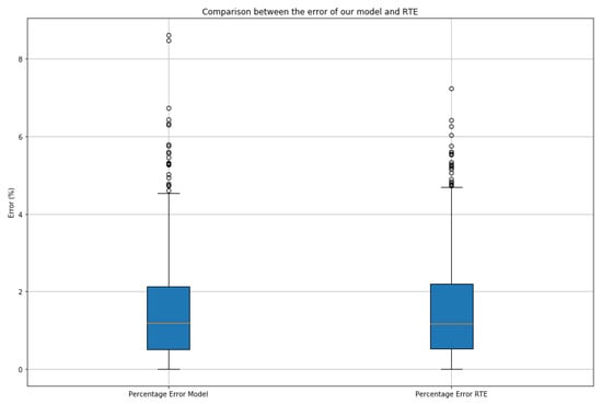
Figure 8.
Absolute percentage error distribution provided by the deep learning structure proposed in this paper and the RTE subscription-based service.
Another interesting measure of the performance of the proposed structure is the absolute percentage error monthly distribution along a full year, as shown in Figure 9.
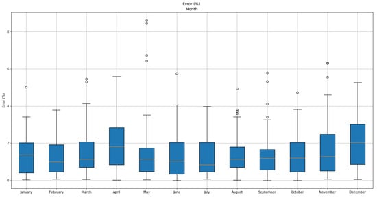
Figure 9.
Absolute percentage error-specific monthly metrics over an entire year as provided by the proposed deep neural network.
In Table 3 and Table 4, the monthly distributed results of the metrics from Equations (1)–(4) are also gathered.
Table 3.
Errors provided by the proposed deep learning structure.
Table 4.
Errors provided by the RTE.
The next Figure 10 depicts the results for the testing of the performance of the forecast provided by the proposed deep neural network on the eight full days extracted from the original data.
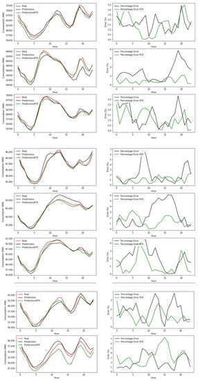
Figure 10.
Performance of the forecast provided by the proposed deep neural network on the eight full days extracted from the original data. (Left column) Real energy consumption, neural network energy prediction and energy prediction by RTE model on a different full day in the Testing Set. (Right column) Absolute Percentage Error in energy prediction throughout the day by the neural network and the model proposed by RTE).
Finally, in order to compare the performance achieved by the approach proposed in this paper with respect to existing solutions, a comparative study was performed. To this end, the CNN + ANN structure was fed with the temperature grid information while the others, which were not specially designed for processing images, were fed with the average temperature values of France. The ARIMA algorithm received as input the past energy demand and predicted that of the future. The results of the experiment are provided in Table 5.
Table 5.
Comparison between the proposed solution and the existing methods.
As the main outcome of the analysis, it can be concluded that the approach that achieved the best results was the deep learning structure presented in this paper, as it showed an improvement even on RTE baseline values. Furthermore, it can be observed that the single ANN, which was only supplied with the average temperature, performed worse than the CNN + ANN method. This fact confirms that the CNN can extract the temperature features for France, providing relevant information to the machine learning algorithm and allowing improved results. Accordingly, the solution presented in this paper was able to enhance the performance of existing methods, thanks to the processing and extraction of features from the French temperature grid performed by the CNN.
4. Discussion
In this paper, the authors presented the adaptation of a deep neural network structure commonly used for image classification applied to the forecast of energy demand. In particular, the structure was trained for the French energy grid.
The results show that the performance of the proposed structure competes with the results provided by the RTE subscription-based reference service. Specifically, the overall MAPE metric of the proposed approach delivers an error of 1.4934%, which is slightly better than the value of 1.4941% obtained with the RTE forecast data.
In addition, a comparison between the proposed solution and existing methods was also performed. As pointed out in the Results section, the suggested approach performed better than all the existing methods which were tested. Specifically, the linear regression, regression tree, and support vector regression (lineal) approaches had a MAPE above 10%, support vector regression (polinomic) had a MAPE of 9.2218%, and ARIMA and ANN had a MAPE that was slightly lower than 3%. Since the MAPE achieved by the proposed structure was 1.4934%, it can be confirmed that the CNN + ANN approach is better than the existing models.
When analyzed on a monthly basis, the errors were uniformly distributed through the year, despite the noticeable increments during the late autumn and winter seasons. This fact is also in accordance with the reference RTE forecast data and may be due to the intermittency of the energy consumption profile observed when French temperatures are low.
The proposed deep neural network also was tested against eight full days randomly selected from the original dataset in order to provide an additional measure of generalization performance. On the one hand and as shown in Figure 10, the errors were uniformly distributed along the selected days. On the other hand, the predictions provided by this paper were quite similar to those predictions provided by the reference RTE subscription service and were also aligned with the overall MAPE metrics. These results indicate that the proposed neural network structure is well designed and trained, and that it generalizes as expected.
The performance achieved in this paper is a promising result for those researchers within the electrical energy industry requiring accurate energy demand forecasting at multiple levels (both temporal and geographical). Despite the focus of this paper on the French macroscopic energy demand problem, the flexibility of the proposed deep neural network and the wide availability of open platforms for its design and training make the proposed approach an accessible and easy-to-implement project. To further facilitate the replication of this paper by other researchers in this area, the authors have included detailed information about the topology and design of the proposed structure.
Author Contributions
Conceptualization, A.J.d.R.; software, F.D.; validation, A.J.d.R. and J.D.; writing—original draft preparation, A.J.d.R.; writing—review and editing, A.J.d.R., F.D. and J.D.; supervision, A.J.d.R. All authors have read and agreed to the published version of the manuscript.
Funding
This research received no external funding.
Conflicts of Interest
The authors declare no conflict of interest.
References
- Hu, H.; Wang, L.; Peng, L.; Zeng, Y.-R. Effective energy consumption forecasting using enhanced bagged echo state network. Energy 2020, 197, 1167–1178. [Google Scholar] [CrossRef]
- Oliveira, E.M.; Luiz, F.; Oliveira, C. Forecasting mid-long term electric energy consumption through bagging ARIMA and exponential smoothing methods. Energy 2018, 144, 776–778. [Google Scholar] [CrossRef]
- Wang, J.; Ma, Y.; Zhang, L.; Gao, R.X.; Wu, D. Deep learning for smart manufacturing: Methods and applications. J. Manuf. Syst. 2018, 48, 144–156. [Google Scholar] [CrossRef]
- RazaKhan, A.; Mahmood, A.; Safdar, A.A.; Khan, Z. Load forecsating, dynamic pricing and DSM in smart grid: A review. Renew. Sustain. Energy Rev. 2016, 54, 1311–1322. [Google Scholar]
- Hippert, H.; Pedreira, C.; Souza, R. Neural Network for short-term load forecasting: A review and evaluation. IEEE Trans. Power Syst. 2001, 16, 44–55. [Google Scholar] [CrossRef]
- Gonzalez-Romera, J.-M.; Carmona-Fernandez, M. Montly electric demand forecasting based on trend extraction. IEEE Trans. Power Syst. 2006, 21, 1946–1953. [Google Scholar] [CrossRef]
- Becalli, M.; Cellura, M.; Brano, L.; Marvuglia, V. Forecasting daily urban electric load profiles using artificial neural networks. Energy Convers. Manag. 2004, 45, 2879–2900. [Google Scholar] [CrossRef]
- Srinivasan, D.; Lee, M.A. Survey of hybrid fuzzy neural approches to a electric load forecasting. In Proceedings of the IEEE international Conference on System, Man and Cybernetics. Intelligent System for the 21st Century, Vancouver, BC, Canada, 22–25 October 1995. [Google Scholar]
- Liu, K.; Subbarayan, S.; Shoults, R.; Manry, M. Comparison of very short-term load forecasting techniques. IEEE Trans. Power Syst. 1996, 11, 877–882. [Google Scholar] [CrossRef]
- Bo, H.; Nie, Y.; Wang, J. Electric load forecasting use a novelty hybrid model on the basic of data preprocessing technique and multi-objective optimization algorithm. IEEE Access 2020, 8, 13858–13874. [Google Scholar] [CrossRef]
- Wen, S.; Wang, Y.; Tang, Y.; Xu, Y.; Li, P.; Zhao, T. Real—Time identification of power fluctuations based on lstm recurrent neural network: A case study on singapore power system. IEEE Trans. Ind. Inform. 2019, 15, 5266–5275. [Google Scholar] [CrossRef]
- Gu, J.; Wangb, Z.; Kuenb, J.; Ma, L.; Shahroudy, A.; Shuaib, B.; Wang, X.; Wang, L.; Wang, G.; Cai, J.; et al. Recent advances in convolutional neural networks. Pattern Recognit. 2017. [Google Scholar] [CrossRef]
- Fukushima, K. Neocognitron: A hierical neural network capable of visual pattern recognition. Neural Netw. 1988, 1, 119–130. [Google Scholar] [CrossRef]
- Alom, M.Z.; Taha, T.M.; Yakopcic, C.; Westberg, S.; Sidike, P. A State-of-the-art survey on deep learning theory and architectures. Electronics 2019, 8, 292. [Google Scholar] [CrossRef]
- Wang, L.; Lu, H.; Ruan, X.; Yang, M.H. Deep networks for saliency detection via local estimation and global search. In Proceedings of the Conference on Computer Vision and Pattern Recognition (CVPR), Boston, MA, USA, 7–12 June 2015. [Google Scholar]
- Jasiński, T. Modeling electricity consumption using nighttime light images and artificial neural networks. Energy 2019, 179, 831–842. [Google Scholar] [CrossRef]
- Kuo, P.-H.; Huang, C.-J. A high precision artificial neural networks model for short-term energy load forecasting. Energies 2018, 11, 213. [Google Scholar] [CrossRef]
- RTE. November 2014. Available online: http://clients.rte-france.com/lang/fr/visiteurs/vie/courbes_methodologie.jsp (accessed on 20 December 2019).
- Arenal Gómez, C. Modelo de Temperatura Para la Mejora de la Predicción de la Demanda Eléctrica: Aplicación al Sistema Peninsular Español; Universidad Politécnica de Madrid: Madrid, Spain, 2016. [Google Scholar]
- ARPEGE. Meteo France, Le Modele. 2019. Available online: https://donneespubliques.meteofrance.fr/client/document/doc_arpege_pour-portail_20190827-_249.pdf (accessed on 3 February 2020).
- Goodfellow, I.; Bengio, Y.; Courville, A. Optimization for training deep models. Deep Learning. 2017, pp. 274–330. Available online: http://faculty.neu.edu.cn/yury/AAI/Textbook/DeepLearningBook.pdf (accessed on 3 February 2020).
- Browlee, J. Machine Learning Mastery. Available online: https://machinelearningmastery.com/weightregularization- (accessed on 3 February 2020).
© 2020 by the authors. Licensee MDPI, Basel, Switzerland. This article is an open access article distributed under the terms and conditions of the Creative Commons Attribution (CC BY) license (http://creativecommons.org/licenses/by/4.0/).