This appendix provides a complete display of the procedure followed to verify the numerical accuracy of the adjoint functions computed. Five specific adjoint functions have been selected for each of the five responses of the model in such a way that, once those have been verified, all the other adjoint functions would be consequently verified as well. For clarity reasons, the adjoint functions have been grouped based on the response they refer to.
Appendix E.1. Verification of the Adjoint Functions for the Outlet Air Temperature Response
When
, the quantities
defined in Equations (21)–(22) all vanish except for a single component, namely:
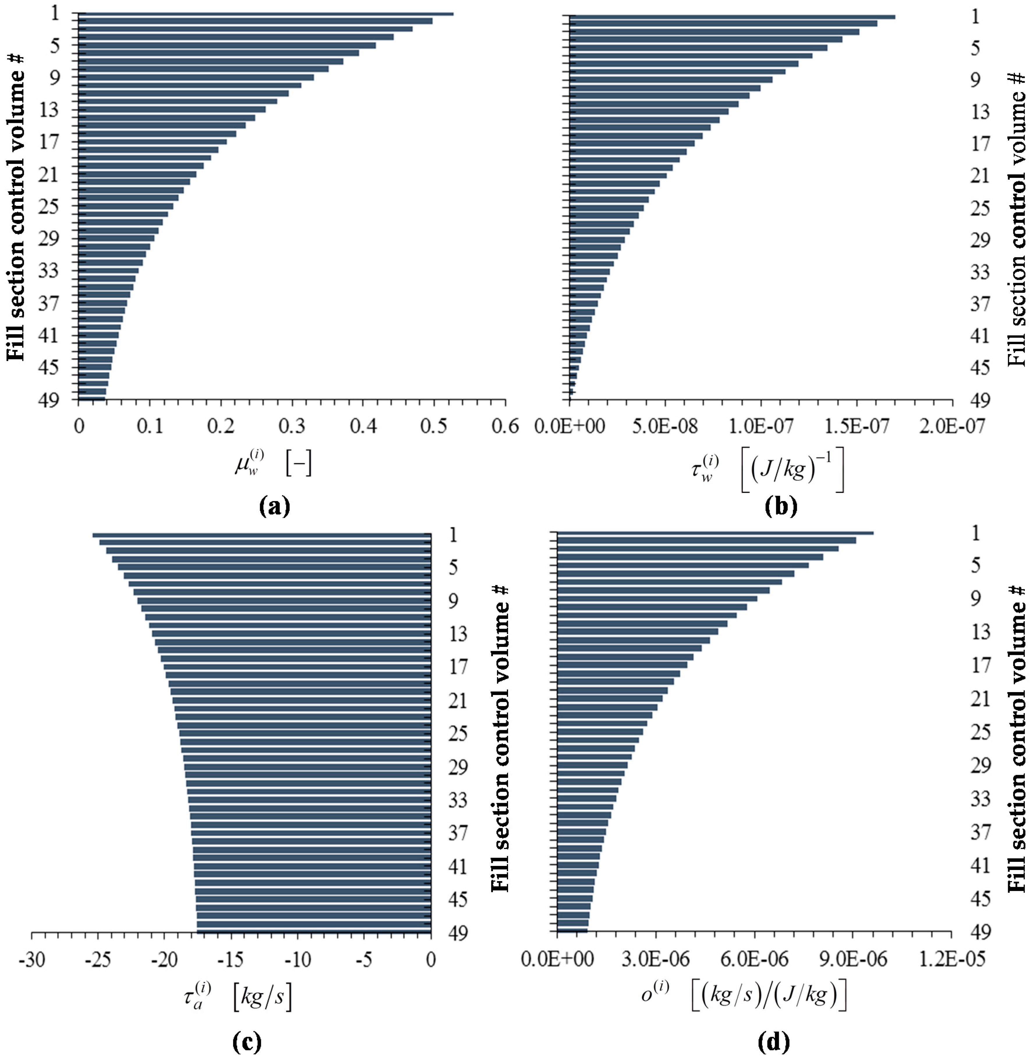
Thus, the adjoint functions corresponding to the outlet air temperature response
are computed by solving the adjoint sensitivity system given in Equation (20) using
as the only non-zero source term; for this case, the solution of Equation (20) has been depicted in
Figure 8.
(a) Verification of the adjoint function
Note that the value of the adjoint function
obtained by solving the adjoint sensitivity system given in Equation (20) is
, as indicated in
Figure 8. Now select a variation
in the wind speed
, and note that Equation (27) yields the following expression for the sensitivity of the response
to
:
Re-writing Equation (E1) in the form
indicates that the value of the adjoint function
could be computed independently if the sensitivity
were available, since the quantity
is known. To first-order in the parameter perturbation, the finite-difference formula given in Equation (28) can be used to compute the approximate sensitivity
; subsequently, this value can be used in conjunction with Equation (E2) to compute a “finite-difference sensitivity” value, denoted as
, for the respective adjoint, which would be accurate up to second-order in the respective parameter perturbation:
Numerically, the wind speed
has the nominal (“base-case”) value of
. The corresponding nominal value
of the response
is
. Consider next a perturbation
, for which the perturbed value of the inlet air temperature becomes
. Re-computing the perturbed response by solving Equations (2)–(14) with the value of
yields the “perturbed response” value
. Using now the nominal and perturbed response values together with the parameter perturbation in the finite-difference expression given in Equation (28) yields the corresponding “finite-difference-computed sensitivity”
. Using this value together with the nominal values of the other quantities appearing in the expression on the right side of Equation (E3) yields
. This result compares well with the value
obtained by solving the adjoint sensitivity system given in Equation (20), cf., below
Figure 8.
The same parameter perturbation was utilized to perform the same verification procedure for the adjoint function
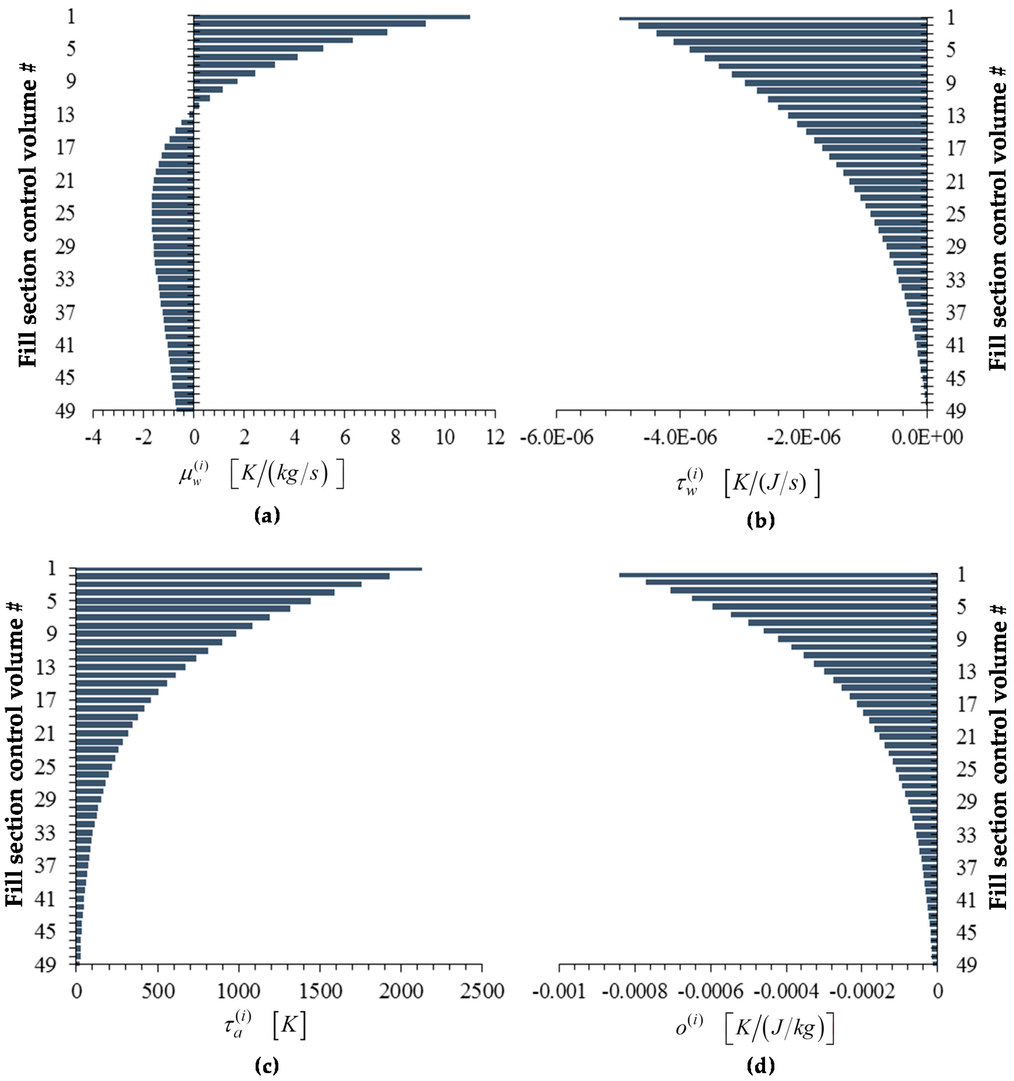
with respect to the other four responses;
Table E1 displays the obtained results, which compare well with the values in the bar plots in
Figure 9,
Figure 10,
Figure 11 and
Figure 12.
Table E1.
Verification Table for adjoint function with respect to the responses and
Table E1.
Verification Table for adjoint function with respect to the responses and
| Response of Interest | | | | | | |
| | | |
| Base case | 1.859 | 298.7979 | −0.27219 | −0.12489 | −0.12651 |
| Perturbed case | 1.84041 | 298.8029 |
| Response of Interest | | | | | | |
| | | |
| Base case | 1.859 | 297.4225 | −0.95514 | −0.43824 | −0.43692 |
| Perturbed case | 1.84041 | 297.4402 |
| Response of Interest | | | | | | |
| | | |
| Base case | 1.859 | 99.79724 | −0.71122 | −0.32632 | -0.33332 |
| Perturbed case | 1.84041 | 99.81046 |
| Response of Interest | | | | | | |
| | | |
| Base case | 1.859 | 43.90797 | −0.073996 | −0.033951 | −0.033873 |
| Perturbed case | 1.84041 | 43.90934 |
| Response of Interest | | | | | | |
| | | |
| Base case | 1.859 | 15.83980 | 11.63149 | 5.33677 | 5.34064 |
| Perturbed case | 1.84041 | 15.62357 |
(b) Verification of the adjoint function
Note that the value of the adjoint function
obtained by solving the adjoint sensitivity system given in Equation (20) is
, as indicated in
Figure 8. Now select a variation
in the inlet air temperature
, and note that Equation (27) yields the following expression for the sensitivity of the response
to
:
Re-writing Equation (E4) in the form
indicates that the value of the adjoint function
could be computed independently if the sensitivity
were available, since the quantities
and
are known. To first-order in the parameter perturbation, the finite-difference formula given in Equation (28) can be used to compute the approximate sensitivity
; subsequently, this value can be used in conjunction with Equation (E5) to compute a “finite-difference sensitivity” value, denoted as
, for the respective adjoint, which would be accurate up to second-order in the respective parameter perturbation:
Numerically, the inlet air temperature
has the nominal (“base-case”) value of
. The corresponding nominal value
of the response
is
. Consider next a perturbation
, for which the perturbed value of the inlet air temperature becomes
. Re-computing the perturbed response by solving Equastions (2)–(14) with the value of
yields the “perturbed response” value
. Using now the nominal and perturbed response values together with the parameter perturbation in the finite-difference expression given in Equation (28) yields the corresponding “finite-difference-computed sensitivity”
. Using this value together with the nominal values of the other quantities appearing in the expression on the right side of Equation (E6) yields
. This result compares well with the value
obtained by solving the adjoint sensitivity system given in Equation (20), cf.,
Figure 8. When solving this adjoint sensitivity system, the computation of
depends on the previously computed adjoint functions
; hence, the forgoing verification of the computational accuracy of
also provides an indirect verification that the functions
were also computed accurately.
The same parameter perturbation was utilized to perform the same verification procedure for the adjoint function
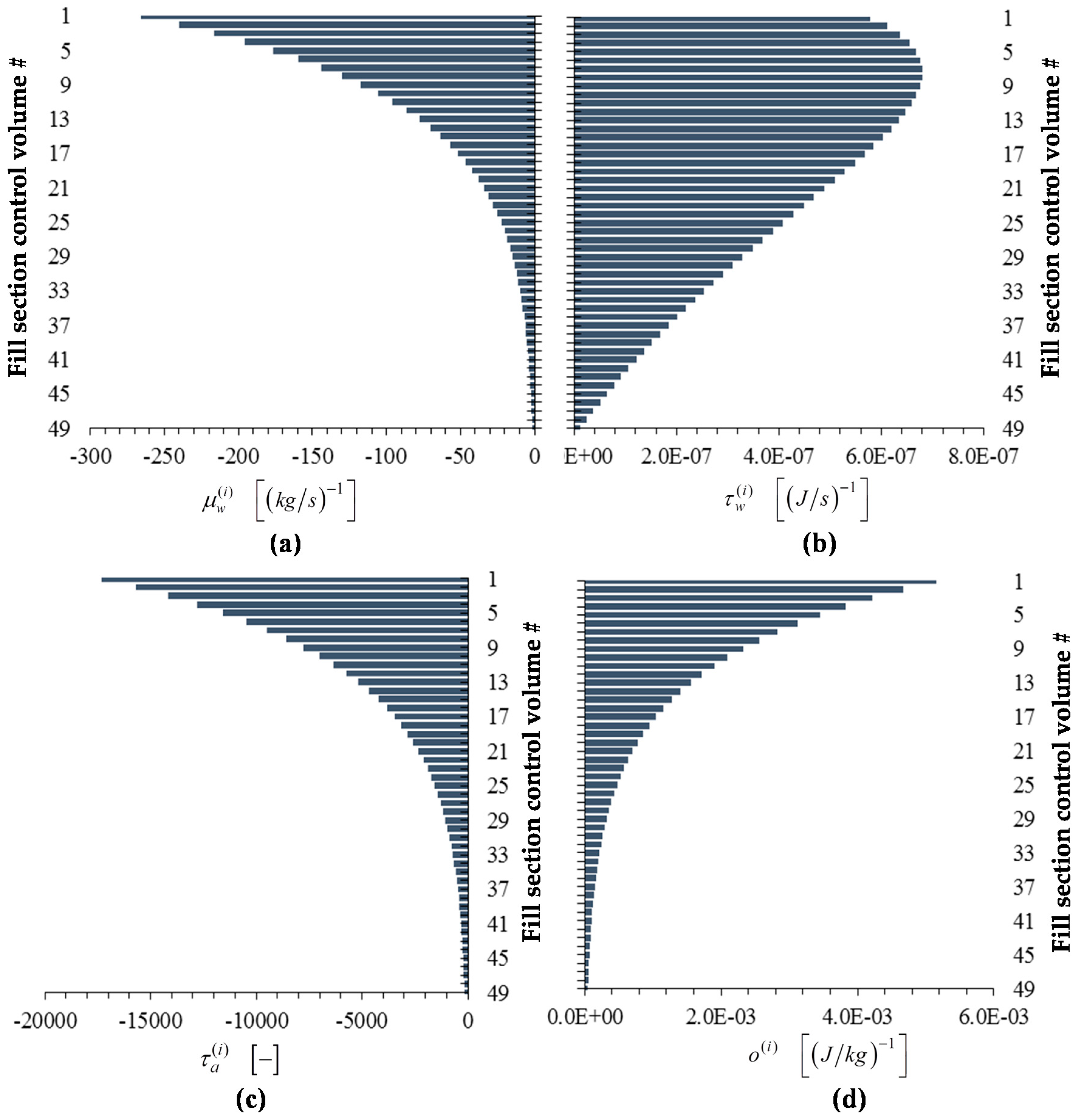
with respect to the other four responses;
Table E2 displays the obtained results, which compare well with the values in the bar plots in
Figure 9,
Figure 10,
Figure 11 and
Figure 12.
Table E2.
Verification Table for adjoint function with respect to the responses and
Table E2.
Verification Table for adjoint function with respect to the responses and
| Response of Interest | | | | | | |
| | | |
| Base case | 298.882 | 298.7979 | 0.06555 | −1.39 × 10⁻⁵ | −1.31 × 10⁻⁵ |
| Perturbed case | 298.852 | 298.7960 |
| Response of Interest | | | | | | |
| | | |
| Base case | 298.882 | 297.4225 | 0.25125 | −7.21 × 10⁻⁵ | −7.28 × 10⁻⁵ |
| Perturbed case | 298.852 | 297.4149 |
| Response of Interest | | | | | | |
| | | |
| Base case | 298.882 | 99.79724 | 0.09039 | 4.32 × 10⁻⁵ | 5.02 × 10⁻⁵ |
| Perturbed case | 298.852 | 99.79453 |
| Response of Interest | | | | | | |
| | | |
| Base case | 298.882 | 43.90797 | 0.012694 | 9.91 × 10⁻⁷ | 9.18 × 10⁻⁷ |
| Perturbed case | 298.852 | 43.90758 |
| Response of Interest | | | | | | |
| | | |
| Base case | 298.882 | 15.83890 | −2.03711 | −1.22 × 10⁻⁴ | −1.18 × 10⁻⁴ |
| Perturbed case | 298.852 | 15.90091 |
(c) Verification of the Adjoint Function
Note that the value of the adjoint function
obtained by solving the adjoint sensitivity system given in Equation (20) is
, as indicated in
Figure 8. Now select a variation
in the inlet air humidity ratio
, and note that Equation (27) yields the following expression for the sensitivity of the response
to
:
Re-writing Equation (E7) in the form
indicates that the value of the adjoint function
could be computed independently if the sensitivity
were available, since the
has been verified in (the previous)
Appendix E.1 (b) and the quantity
is known. To first-order in the parameter perturbation, the finite-difference formula given in Equation (28) can be used to compute the approximate sensitivity
; subsequently, this value can be used in conjunction with Equation (E8) to compute a “finite-difference sensitivity” value, denoted as
, for the respective adjoint, which would be accurate up to second-order in the respective parameter perturbation:
Numerically, the inlet air humidity ratio
has the nominal (“base-case”) value of
. The corresponding nominal value
of the response
is
. Consider next a perturbation
, for which the perturbed value of the inlet air humidity ratio becomes
. Re-computing the perturbed response by solving Eqsuations (2)–(14) with the value of
yields the “perturbed response” value
. Using now the nominal and perturbed response values together with the parameter perturbation in the finite-difference expression given in Equation (28) yields the corresponding “finite-difference-computed sensitivity”
. Using this value together with the nominal values of the other quantities appearing in the expression on the right side of Equation (E9) yields
. This result compares well with the value
obtained by solving the adjoint sensitivity system given in Equation (20), cf.
Figure 8. When solving this adjoint sensitivity system, the computation of
depends on the previously computed adjoint functions
; hence, the forgoing verification of the computational accuracy of
also provides an indirect verification that the functions
were also computed accurately.
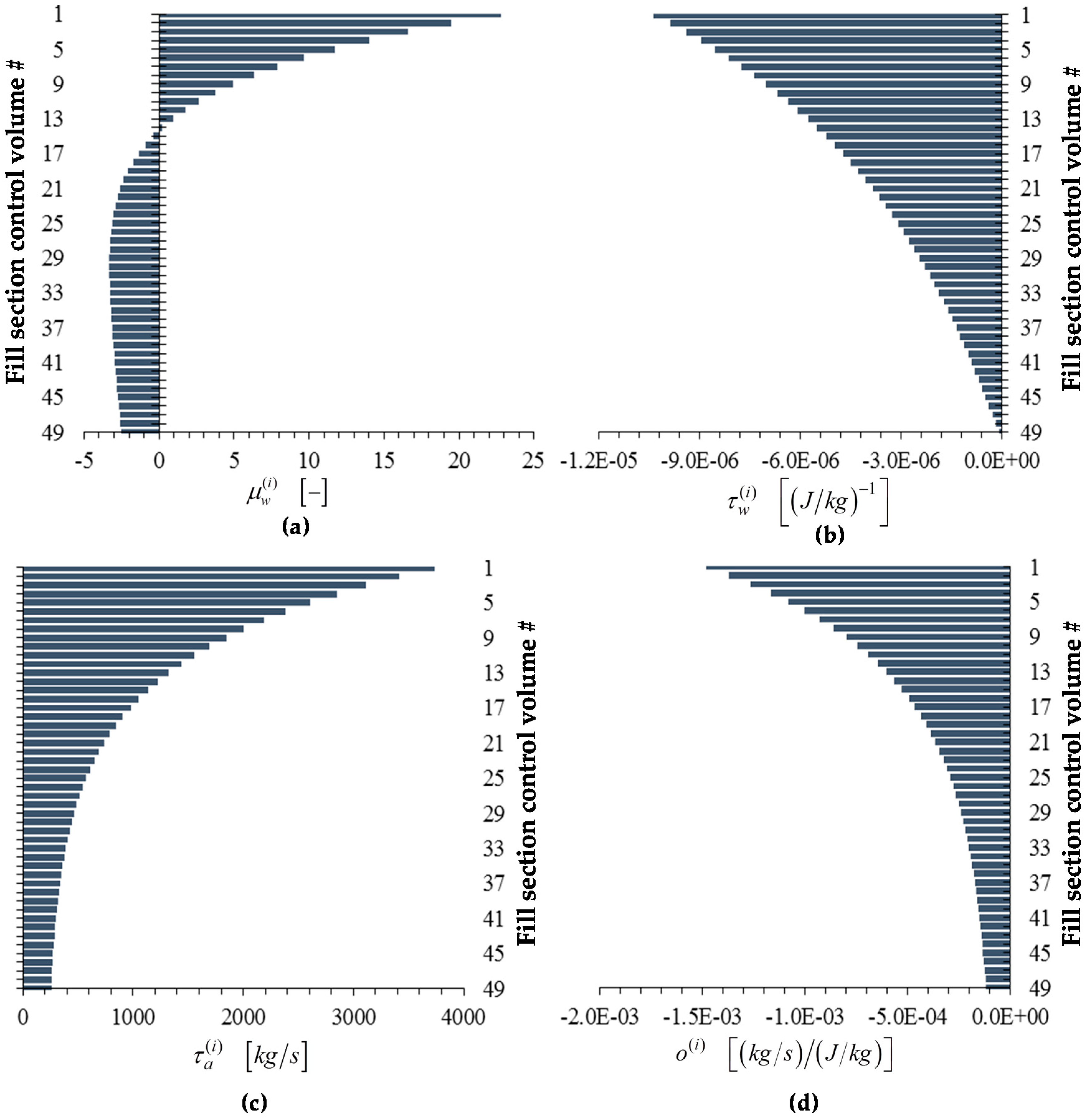
The same parameter perturbation was utilized to perform the same verification procedure for the adjoint function
with respect to the other four responses;
Table E3 displays the obtained results, which compare well with the values in the bar plots in
Figure 9,
Figure 10,
Figure 11 and
Figure 12.
Table E3.
Verification Table for adjoint function with respect to the responses and
Table E3.
Verification Table for adjoint function with respect to the responses and
| Response of Interest | | | | | | |
| | | |
| Base case | 0.0137976 | 298.7979 | 11.878 | 21.569 | 21.555 |
| Perturbed case | 0.0137803 | 298.7977 |
| Response of interest | | | | | | |
| | | |
| Base case | 0.0137976 | 297.4225 | 201.180 | −15.593 | −15.799 |
| Perturbed case | 0.0137803 | 297.4190 |
| Response of interest | | | | | | |
| | | |
| Base case | 0.0137976 | 99.79724 | 24.4676 | −152.46 | −152.50 |
| Perturbed case | 0.0137803 | 99.79681 |
| Response of interest | | | | | | |
| | | |
| Base case | 0.0137976 | 43.90797 | 15.1936 | −17.533 | −17.549 |
| Perturbed case | 0.0137803 | 43.90770 |
| Response of interest | | | | | | |
| | | |
| Base case | 0.0137976 | 15.83890 | 43.92139 | 256.109 | 256.059 |
| Perturbed case | 0.0137803 | 15.83903 |
(d) Verification of the adjoint functions
Note that the values of the adjoint function
obtained by solving the adjoint sensitivity system given in Equation (20) is as follows:
, as indicated in
Figure 8. Now select a variation
in the inlet water temperature
, and note that Equation (27) yields the following expression for the sensitivity of the response
to
:
Re-writing Equation (E10) in the form
indicates that the value of the adjoint function
could be computed independently if the sensitivity
were available, since the quantity
is known. To first-order in the parameter perturbation, the finite-difference formula given in Equation (28) can be used to compute the approximate sensitivity
; subsequently, this value can be used in conjunction with Equation (E11) to compute a “finite-difference sensitivity” value, denoted as
, for the respective adjoint, which would be accurate up to second-order in the respective parameter perturbation:
Numerically, the inlet water temperature,
, has the nominal (“base-case”) value of
. As before, the corresponding nominal value
of the response
is
. Consider now a perturbation
, for which the perturbed value of the inlet air temperature becomes
. Re-computing the perturbed response by solving Equations (2)–(14) with the value of
yields the “perturbed response” value
. Using now the nominal and perturbed response values together with the parameter perturbation in the finite-difference expression given in Equation (28) yields the corresponding “finite-difference-computed sensitivity”
. Using this value together with the nominal values of the other quantities appearing in the expression on the right side of Equation (E12) yields
. This result compares well with the value
obtained by solving the adjoint sensitivity system given in Equation (20), cf.
Figure 8.
The same parameter perturbation was utilized to perform the same verification procedure for the adjoint function
with respect to the other four responses;
Table E4 displays the obtained results, which compare well with the values in the bar plots in
Figure 9,
Figure 10,
Figure 11 and
Figure 12.
Table E4.
Verification Table for adjoint function with respect to the responses and
Table E4.
Verification Table for adjoint function with respect to the responses and
| Response of Interest | | | | | | |
| | | |
| Base case | 298.893 | 298.7979 | 0.91889 | −4.99 × 10⁻⁶ | −4.98 × 10⁻⁶ |
| Perturbed case | 298.873 | 298.7795 |
| Response of interest | | | | | | |
| | | |
| Base case | 298.893 | 297.4225 | 0.50358 | −2.73 × 10⁻⁶ | −2.73 × 10⁻⁶ |
| Perturbed case | 298.873 | 297.4124 |
| Response of interest | | | | | | |
| | | |
| Base case | 298.893 | 99.79724 | −0.10693 | 5.77 × 10⁻⁷ | 5.78 × 10⁻⁷ |
| Perturbed case | 298.873 | 99.7994 |
| Response of interest | | | | | | |
| | | |
| Base case | 298.893 | 43.90797 | −0.031364 | 1.70 × 10⁻⁷ | 1.70 × 10⁻⁷ |
| Perturbed case | 298.873 | 43.90859 |
| Response of interest | | | | | | |
| | | |
| Base case | 298.893 | 15.83980 | 1.91042 | −1.037 × 10⁻⁵ | −1.035 × 10⁻⁵ |
| Perturbed case | 298.873 | 15.80159 |
(e) Verification of the adjoint function
Note that the values of the adjoint function
obtained by solving the adjoint sensitivity system given in Equation (20) is as follows:
, as indicated in
Figure 8. Now select a variation
in the inlet water mass flow rate
, and note that Equation (27) yields the following expression for the sensitivity of the response
to
:
Since the adjoint functions
and
have been already verified as described in
Appendix E.1 (b) and
Appendix E.1 (c), it follows that the computed values of adjoint functions
can also be considered as being accurate, since they constitute the starting point for solving the adjoint sensitivity system in Equation (20);
was proved being accurate in
Appendix E.1 (d).
Re-writing Equation (E13) in the form
indicates that the value of the adjoint function
could be computed independently if the sensitivity
were available, since all the other quantities are known. To first-order in the parameter perturbation, the finite-difference formula given in Equation (28) can be used to compute the approximate sensitivity
; subsequently, this value can be used in conjunction with Equation (E14) to compute a “finite-difference sensitivity” value, denoted as
, for the respective adjoint, which would be accurate up to second-order in the respective parameter perturbation:
Numerically, the inlet water mass flow rate,
, has the nominal (“base-case”) value of
. As before, the corresponding nominal value
of the response
is
. Consider now a perturbation
, for which the perturbed value of the inlet air temperature becomes
. Re-computing the perturbed response by solving Equations (2)–(14) with the value of
yields the “perturbed response” value
. Using now the nominal and perturbed response values together with the parameter perturbation in the finite-difference expression given in Equation (28) yields the corresponding “finite-difference-computed sensitivity”
. Using this value together with the nominal values of the other quantities appearing in the expression on the right side of Equation (E15) yields
. This result compares well with the value
obtained by solving the adjoint sensitivity system given in Equation (20), cf.
Figure 8.
The same parameter perturbation was utilized to perform the same verification procedure for the adjoint function
with respect to the other four responses;
Table E5 displays the obtained results, which compare well with the values in the bar plots in
Figure 9,
Figure 10,
Figure 11 and
Figure 12.
Table E5.
Verification Table for adjoint function with respect to the responses and
Table E5.
Verification Table for adjoint function with respect to the responses and
| Response of Interest | | | | | | |
| | | |
| Base case | 44.0193 | 298.7979 | 0.00328 | 10.977 | 10.301 |
| Perturbed case | 43.9893 | 298.7978 |
| Response of Interest | | | | | | |
| | | |
| Base case | 44.0193 | 297.4225 | 0.03142 | 6.0444 | 6.0443 |
| Perturbed case | 43.9893 | 297.4215 |
| Response of Interest | | | | | | |
| | | |
| Base case | 44.0193 | 99.79724 | −0.001267 | −265.511 | −265.511 |
| Perturbed case | 43.9893 | 99.79728 |
| Response of interest | | | | | | |
| | | |
| Base case | 44.0193 | 43.90797 | 0.99986 | 0.52753 | 0.52753 |
| Perturbed case | 43.9893 | 43.87797 |
| Response of Interest | | | | | | |
| | | |
| Base case | 44.0193 | 15.83980 | 0.010543 | 22.807 | 22.807 |
| Perturbed case | 43.9893 | 15.83948 |


