Pine-YOLO: A Method for Detecting Pine Wilt Disease in Unmanned Aerial Vehicle Remote Sensing Images

Abstract

Pine wilt disease is a highly contagious forest quarantine ailment that spreads rapidly. In this study, we designed a new Pine-YOLO model for pine wilt disease detection by incorporating Dynamic Snake Convolution (DSConv), the Multidimensional Collaborative Attention Mechanism (MCA), and Wise-IoU v3 (WIoUv3) into a YOLOv8 network. Firstly, we collected UAV images from Beihai Forest and Linhai Park in Weihai City to construct a dataset via a sliding window method. Then, we used this dataset to train and test Pine-YOLO. We found that DSConv adaptively focuses on fragile and curved local features and then enhances the perception of delicate tubular structures in discolored pine branches. MCA strengthens the attention to the specific features of pine trees, helps to enhance the representational capability, and improves the generalization to diseased pine tree recognition in variable natural environments. The bounding box loss function has been optimized to WIoUv3, thereby improving the overall recognition accuracy and robustness of the model. The experimental results reveal that our Pine-YOLO model achieved the following values across various evaluation metrics: [email protected] at 90.69%, [email protected]:0.95 at 49.72%, precision at 91.31%, recall at 85.72%, and F1-score at 88.43%. These outcomes underscore the high effectiveness of our model. Therefore, our newly designed Pine-YOLO perfectly addresses the disadvantages of the original YOLO network, which helps to maintain the health and stability of the ecological environment.

1. Introduction

Pine trees are widely distributed worldwide and primarily grow in the temperate regions of the Northern Hemisphere, such as Russia, Canada, the United States, China, Japan, and Sweden. Pine trees are highly significant arboreal species inside the forest, fulfilling a crucial function in safeguarding the ecosystem and upholding the equilibrium of carbon levels. Nevertheless, pine trees are always vulnerable to infestations and illnesses. Pine wilt disease is a highly contagious forest quarantine ailment that spreads rapidly and causes significant mortality [1]. This disease is transmitted both artificially and naturally. Artificial transmission refers to the movement of contaminated wood and its products, as well as the utilization of infected wood as packaging in commercial transactions [2]. Natural transmission is mainly generated by the spread of the infection to new pine trees by monochamus and other insect vectors [3]. This vector is native to North America, but its distribution and damage range have been expanded dramatically to many countries such as China, Japan, Korea, Portugal, and Spain [4]. The pine wood nematode has been spreading in China as an invasive species since 1982, resulting in the mortality of significant numbers of pine trees [5]. This reduces forest carbon sinks continuously and thus brings huge economic losses to the world [6]. The primary strategies to prevent the further dissemination of the pine wood nematode include physical control, chemical control, and biological control. The first two methods are the most efficient but are harmful to the ecological environment, and biological control takes too long a time to achieve efficient control. Most importantly, all these three methods need precise surveillance of infected trees to treat them effectively and promptly.

There are three main means to monitor the pine wilt disease, namely, manual inspection, satellite or aerial remote sensing monitoring, and unmanned aerial vehicle (UAV) monitoring. Manual inspections are labor-intensive, inefficient, and costly, and are further constrained by the uneven geographical distribution of pine trees and the complex and variable environments in which they are situated [7,8]. Satellite or aerial remote sensing monitoring can achieve large-area spatial coverage, but they are limited by sensor resolution and satellite operation cycles. UAV remote sensing has been increasingly used in agriculture and forestry with advantages such as higher flexibility, lower cost, and higher resolution relative to satellite remote sensing, etc. [9,10]. Remote sensing plays a crucial role in the detection of forest health.

To process the massive remote-sensing images of pine trees acquired by satellites or UAV, machine learning has been extensively used and developed. Syifa et al. [11] divided the images based on GPS into classes such as PWD-indicated trees, normal pine, buildings, roads. Their study has enhanced the ability to distinguish buildings or roads with similar colors to PWD-indicated trees. Oide et al. [12] combined visible color imagery and ML algorithms, but were not concerned with detecting the infection stages of individual trees. In order to detect PWD earlier, Iordache et al. [13] and Yu et al. [14] assigned infected trees to different classes and distinguished early infections from other stages. Wu et al. [15] proposed the green attack stage as the key issue for early monitoring and compared the differences in detection accuracy across different dates. Traditional machine learning must construct data features manually with high separability and select appropriate classifiers, which are not suitable for large-scale data training. Machine learning also struggles to adapt to diverse and complex scenarios, resulting in limited practicality. For instance, overlapping tree canopies make it difficult to distinguish the target from surrounding trees, and similar-colored backgrounds and other dead trees cause detection confusion.

Unlike traditional machine learning, deep learning algorithms are adapted to training on large-scale raw datasets and various complex scenarios. Therefore, it has been applied to remote sensing more widely due to its powerful automatic feature learning without human intervention. It is a common practice to employ diverse methods to enhance remote sensing images, such as mirroring, flipping, adding noise, rotating, scaling, etc. [16,17,18]. Cai et al. [19] proposed an effective data augmentation method based on Sentinel-2 satellite data and UAV images to efficiently detect PWD. Zhang et al. [20] corrected 5-band multi-spectral images and visualized them as heat maps to propose a patch-based deep classification. Many researchers also engage in evaluating [21,22] or improving models [23,24,25,26,27,28], such as optimizing neural networks. Deng et al. [29] improved Faster-RCNN based on RPN and added a geographic location module. Li et al. [30] proposed YOLOv4-Tiny-3Layers to filter uninterested and irrelevant images. Abdollahnejad et al. [31] innovatively used UAV images as reference data and combines high-resolution satellite platforms with time series data to evaluate and predict forest health status. Ren et al. [32] proposed a Global Multi-Scale Channel Adaptation Network based on circle sampling to better match the circular shape of the diseased trees. Zhang et al. [33] improved YOLOv5 by four attention mechanism modules to detect smaller infected wood in images that covers a large area. Qin et al. [34] designed SCANet (spatial-context-attention network) and Han et al. [35] proposed multi-scale spatial supervision convolutional network (MSSCN) to reduce the loss of spatial information and detect trees in complex backgrounds.

In comparison, YOLO has greatly enhanced the speed of detection. Additionally, it excels in learning generalized features of detection targets, thereby reducing background recognition errors. While extensive researches have been conducted to apply YOLO in identification of pine wilt disease, challenges still remain, including accurate detection in complex backgrounds, identifying subtle tubular structures in pine tree branches, etc. Inspired by previous research, we adopted the highly precise and adaptable YOLOv8 model as our benchmark network and developed a new detection model named Pine-YOLO. This model integrates DSConv (Dynamic Snake Convolution) and incorporates MCA (Multidimensional Collaborative Attention Mechanism) along with WIoUv3 (Wise-IoU v3). We acquired images of pine forests in the Weihai area via the UAV remote sensing technique, then used these data to train and evaluate the new Pine-YOLO model. Finally, we found this new model can effectively extract fine and curved structures in a complex natural environment, so it can reach an extreme high accuracy of ~90%.

2. Materials and Methods

2.1. Image Acquisition

In this work, we utilized images from Beihai Forest and Linhai Park, located in Weihai City (37°30′ N, 122°6′ E), Shandong Province, China. More than 70% of the vegetation in this area is made up of pine trees, and some of them are already nematode-infected, which is depicted in Figure 1.

The research area boasts an extensive coastline, is situated in the north temperate zone, and is characterized by a monsoon continental climate, with black pine being the predominant species. The research area exhibits a rich age structure, encompassing various growth stages from seedlings to mature trees. Vertically, the forest can be divided into three main layers: the uppermost layer consists of mature, tall pine trees forming the canopy; the middle layer is primarily composed of mid-height pine trees and a few other tree species, adding to the forest’s vertical complexity; the ground layer is dominated by shrubs and herbaceous plants. Horizontally, the distribution of trees within the forest is not uniform but rather presents a pattern of dense areas and open spaces alternating, indicating a high level of structural complexity in the forest.

A DaJiang UAV outfitted with a DG2pro CMOS was employed as a flying platform in the data gathering procedure, conducting six flights at altitudes ranging from 180 m to 240 m. The sizes of these orthorectified images are 128,601 × 62,669 pixels, 126,365 × 90,989 pixels, 48,236 × 47,168 pixels, and 57,653 × 48,979 pixels, respectively, amounting to a total coverage area of approximately 22.19 km². Using a custom program which we developed and compiled in PyCharm, the original images are segmented into 43,095 image slices in 1024 × 1024 pixels by a sliding window method with 20% overlapping area, which is demonstrated in Figure 2b. The geographic coordinates of all diseased pine tree samples are individually labeled and verified on-site. During the training process, the image dataset containing diseased pine trees is randomly divided into a training dataset and a validation dataset in a ratio of 8:2. The dataset collection was conducted between 27 September–8 October 2022, during which the weather was predominantly cloudy, with two days of rainfall. The strategic selection of this period aimed to mitigate the confounding effects of drought stress and discoloration observed in deciduous broad-leaved trees. This timing not only avoids the phenotypic variations commonly induced by environmental stressors, but also ensures the specificity of the phenotypic features associated with pine wilt disease (PWD) in our study. Careful selection of the dataset during this period further helped in minimizing the inclusion of tubular, locally elongated, and curved branch structures that might arise from conditions other than PWD, thereby enhancing the detection accuracy of our improved method focusing on tubular structural enhancements.

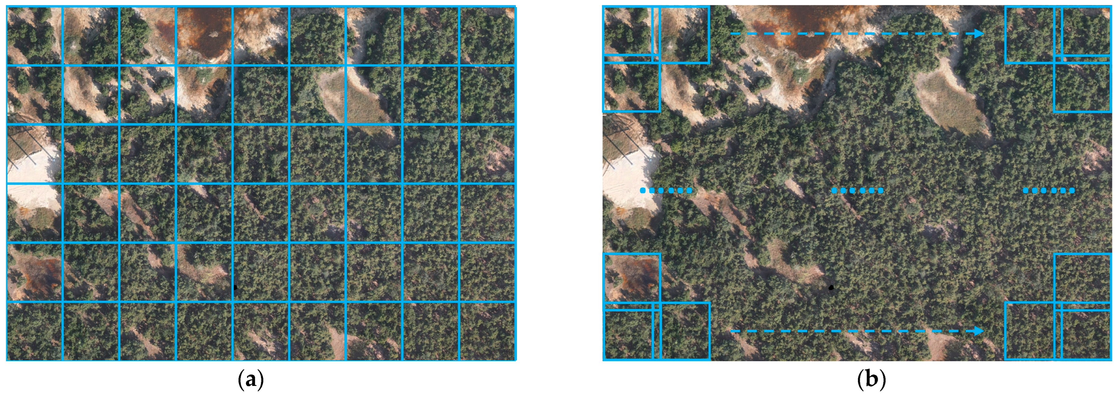
2.2. Image Pre-Processing

In this study, we adopt the mosaic data pre-processing technique integrated within the YOLOv8 framework to augment the variety of the training dataset, thereby strengthening the generalization ability of this model. This technique randomly combines four different photos into a unified image by stochastic scaling, cropping, and alignment processes, as illustrated in Figure 3. This approach not only adds new variations to the small-sized targets in the training sample, but also helps to achieve a balanced distribution for the labeled diseased and unlabeled diseased pine trees in the dataset.

2.3. Detection Networks

2.3.1. Pine-YOLO Network Structure

YOLOv8 shows excellent detection speed and accuracy, and it is composed of four key components: the Input module, Backbone module, Neck module, and Head module. The Input module primarily utilizes techniques like mosaic data augmentation, dynamic anchor box computation and grayscale augmentation, etc. The Backbone module includes Conv, C2f, and SPPF, etc., where C2f learns residual features and expands the model gradient flow by branching across layer connections. The Neck module still uses the PAN-FPN idea to enhance the fusion of object features in different dimensions. The Head module adopts a decoupled head structure that calculates the confidence and location of the final detected target based on the enhanced features [36].

In detection of pine wilt disease, the morphologic features of the dataset are a critical factor to obtain perfect recognition results. However, images of diseased pine trees taken via UAV remote sensing are particularly sensitive to variations in lighting and shadow conditions; some infected pine trees also have color and texture differences. Therefore, when the standard YOLOv8 network is employed to perform the detection of pine wilt disease using UAV remote sensing images, it usually outputs a significant number of false negative and false positive results. To address these disadvantages, we integrated the DSConv module into the YOLOv8 network in this study, along with the MCA module and the WIoUv3 loss function, thus developing a new Pine-YOLO model. This newly designed model improves the ability of feature extraction from pine trees and image recognition amidst background interference, thereby reducing the false negatives and false positives in the whole training and testing processes. The network structure of Pine-YOLO is shown in Figure 4.

2.3.2. Dynamic Snake Convolution (DSConv)

In the overhead view of the UAV remote sensing images, we noted that in addition to the obvious color features, the branches of diseased pine trees are topologically tubular, locally elongated, and curved.

As shown in Figure 5, YOLOv8 is able to learn geometric variations freely by the addition of DSConv, because the perception of geometric structures is improved by adaptively focusing on the fragile and curved local features of the tubular structure. On fine tubular structures, this approach can consider the serpentine morphology of the tubular structure and use constraints to complement the free learning process to enhance the perception of fine tubular structures in discolored pine branches [37].

DSConv enhances target recognition using deformation offsets. This allows the convolutional kernel to flexibly focus on the complex and variable geometric features of the target. Additionally, an iterative strategy is employed in this model to prevent the perceptual field from drifting away from the target during the free learning of these deformation offsets. This strategy involves selecting the subsequent target for observation in the processing sequence, which ensures continuity of attention while not extending the perceptual range further, due to the excessive deformation offsets.

DSConv, introduced here, defines a convolution kernel G with size 9 in the x-axis and y-axis directions, and the distinct portrayal of each network in G is $G_{i\pm a}=\left(x_{i\pm a},y_{i\pm a}\right)$, where $a=\{0, 1, 2, 3, 4\}$ represents the horizontal distance between the grid and the central location, whereas the choice of each grid point $G_{i\pm a}$ in the convolution kernel G_i is an accumulative procedure. Starting from G_i, the position away from the center grid depends on the position of the previous grid: $G_{i\pm a}$ has an additional offset $\Delta =\{\delta \mid \delta \in [-\mathrm{1,1}\left]\right\}$ compared to G_i. Therefore, the offset needs to be Σ in order to ensure that the convolution kernel adheres to a linear structural shape. As shown in Figure 6, G_i±a in the x-axis direction becomes:

$$G_{i\pm a}=\left\{\begin{array}{c}\left(x_{i+a},y_{i+a}\right)=\left(x_i+a,y_i+{\Sigma }_i^{i+a}\Delta y\right)\\ \left(x_{i-a},y_{i-a}\right)=\left(x_i-a,y_i+{\Sigma }_{i-a}^i\Delta y\right)\end{array}\right.$$

(1)

G_i±a in the y-axis direction becomes:

$$G_{j\pm a}=\left\{\begin{array}{c}\left(x_{j+a},y_{j+a}\right)=\left(x_j+{\Sigma }_j^{j+a}\Delta x,y_j+a\right)\\ \left(x_{j-a},y_{j-a}\right)=\left(x_j+{\Sigma }_{j-a}^j\Delta x,y_j-a\right)\end{array}\right.$$

(2)

The bilinear interpolation formula is written as follows:

$$G={\displaystyle {\Sigma }_{G^{\prime }}}D\left(G^{\prime },G\right)\cdot G^{\prime }$$

(3)

where G is the fractional portion of Equations (1) and (2), $G^{\prime }$ enumerates all integral space positions, and D is a bilinear interpolation kernel being divided into two one-dimensional kernels:

$$D\left(G,G^{\prime }\right)=d\left(G_x,G{\prime }_x\right)\cdot d\left(G_y,{G^{\prime }}_y\right)$$

(4)

As shown in Figure 6, due to the two-dimensional (x-axis, y-axis) variations, DSConv covers a 9 × 9 range during deformation to acquire better adaptability to the slender tubular structures on top of the dynamic structure, improving the perception of key features.

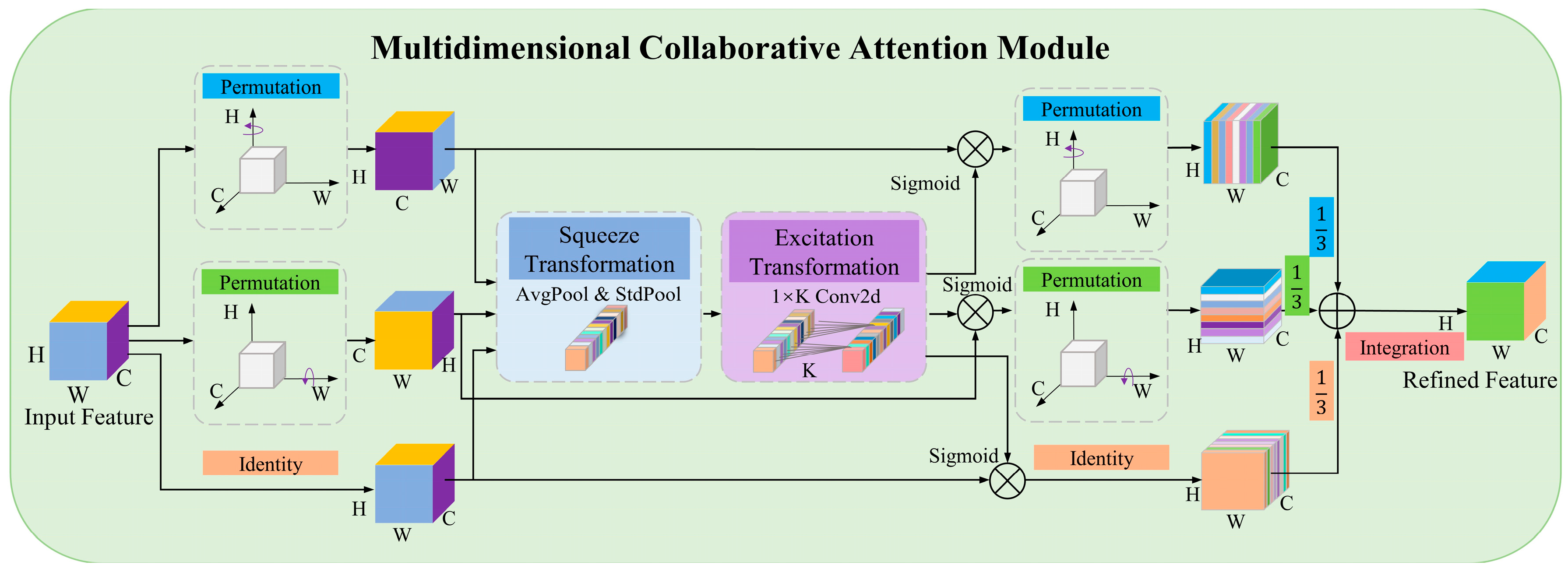
2.3.3. Multidimensional Collaborative Attention Mechanism

The multidimensional collaborative attention mechanism (MCA) successfully captures the spatial dimension and feature interdependence between channels through its parallel branching structure, and thus enhances the comprehension of the YOLOv8 model of the spatial properties of pine trees and their representations in images. At the same time, MCA also strengthens the attention on the specific features of pine trees by fine-tuning the input feature maps. This can raise the accuracy of recognition, specifically in cases where the background is complex or the pine tree features are not obvious. This attention can also provide efficient performance gains by enhancement of the network representation, improving the generalization of the model for pine tree recognition, which is valuable in variable natural environments.

As shown in Figure 7, the MCA module we used comprises three branches. Each branch is dedicated to a separate attentional model in the channel, width, and height dimensions. The squeeze transformation employs global mean and standard deviation pooling to consolidate cross-dimensional feature responses. It also employs a combinatorial technique to intelligently blend mean and standard deviation pool information, hence improving the representation of feature descriptors. The excitation transformation structure of MCA effectively resolves the dilemma between detection performance and computational overhead trade-offs by dynamically capturing local feature interactions.

The uppermost branch is utilized to record the interconnections among characteristics in the spatial dimension W. Similarly, the middle branch is utilized to record the relationships between features in the spatial dimension H. The lower branch obtains the exchanges among channels. The MCA utilizes substitution procedures to capture the long-term dependencies between the channel dimension and either of the spatial dimensions in the first two branches. Ultimately, the results from each of the three branches are combined by a straightforward averaging process during the integration step. The symbol $\otimes$ in Figure 7 denotes broadcast element multiplication, and $\oplus$ denotes broadcast element summation. The overall design intends to convert input features into fine outputs of the same dimensions.

MCA can also be viewed as a computational unit that performs specific transformations to refine the input tensor into an output tensor of the same shape. Specifically, let F denote the outcome of the convolutional layer and functions as the input feature mapping for the MCA module; then, the shape of F can be described as C × H × W, where C, H, and W refer to the number of channels (filters), the height and width of the spatial feature map, respectively. The purpose of the MCA module is to feed F into each branch to enhance its refining feature. F performs $T_{\mathit{trans}}$ on three branches separately. We should note that F is rotated 90° anticlockwise along both the H-axis and W-axis in the first branch and the second branch, while the original features are maintained after$T_{\mathit{trans}}$ in the third branch, generating the feature map denoted as $\stackrel{⏜}{\mathit{F}}$. Then, $\stackrel{⏜}{\mathit{F}}$ is input into the squeeze transformation to obtain the aggregated feature map $\widehat{\mathit{F}}$. Then, $\widehat{\mathit{F}}$ is passed into the excitation transformation to capture the spatial dimensions and inter-channel feature interactions, producing $\tilde{\mathit{F}}$ accordingly. Next, $\tilde{\mathit{F}}$ is passed through the sigmoid activation function and A is applied to $\stackrel{⏜}{\mathit{F}}$ via element-by-element multiplication to obtain the enhanced feature map ${\mathit{F}}^{\prime }$. Finally, ${\mathit{F}}^{\prime }$ is inverted by $T_{\mathit{trans}}$ to obtain ${\mathit{F}}^{″}$. This process can be summarized in the following equations:

$$\stackrel{⏜}{\mathit{F}}=T_{\mathit{trans}}(\mathit{F})$$

(5)

$$\widehat{\mathit{F}}=T_{sq}\left(\stackrel{⏜}{\mathit{F}}\right), \tilde{\mathit{F}}=T_{ex}\left(\widehat{\mathit{F}}\right)$$

(6)

$$\mathcal{A}=\sigma \left(\tilde{\mathit{F}}\right), {\mathit{F}}^{\prime }=\mathcal{A}\otimes \stackrel{⏜}{\mathit{F}}, {\mathit{F}}^{″}=T_{trans}^{-1}\left({\mathit{F}}^{\prime }\right)$$

(7)

where $T_{trans}(\cdot )$ denotes the transformation of the input feature map, while $T_{trans}^{-1}(\cdot )$ denotes the inverse transformation process, $\sigma (\cdot )$ represents the sigmoid activation function, $T_{sq}(\cdot )$ and $T_{\mathit{ex}}(\cdot )$ denote the squeezing and excitation transforms, respectively.

(1)

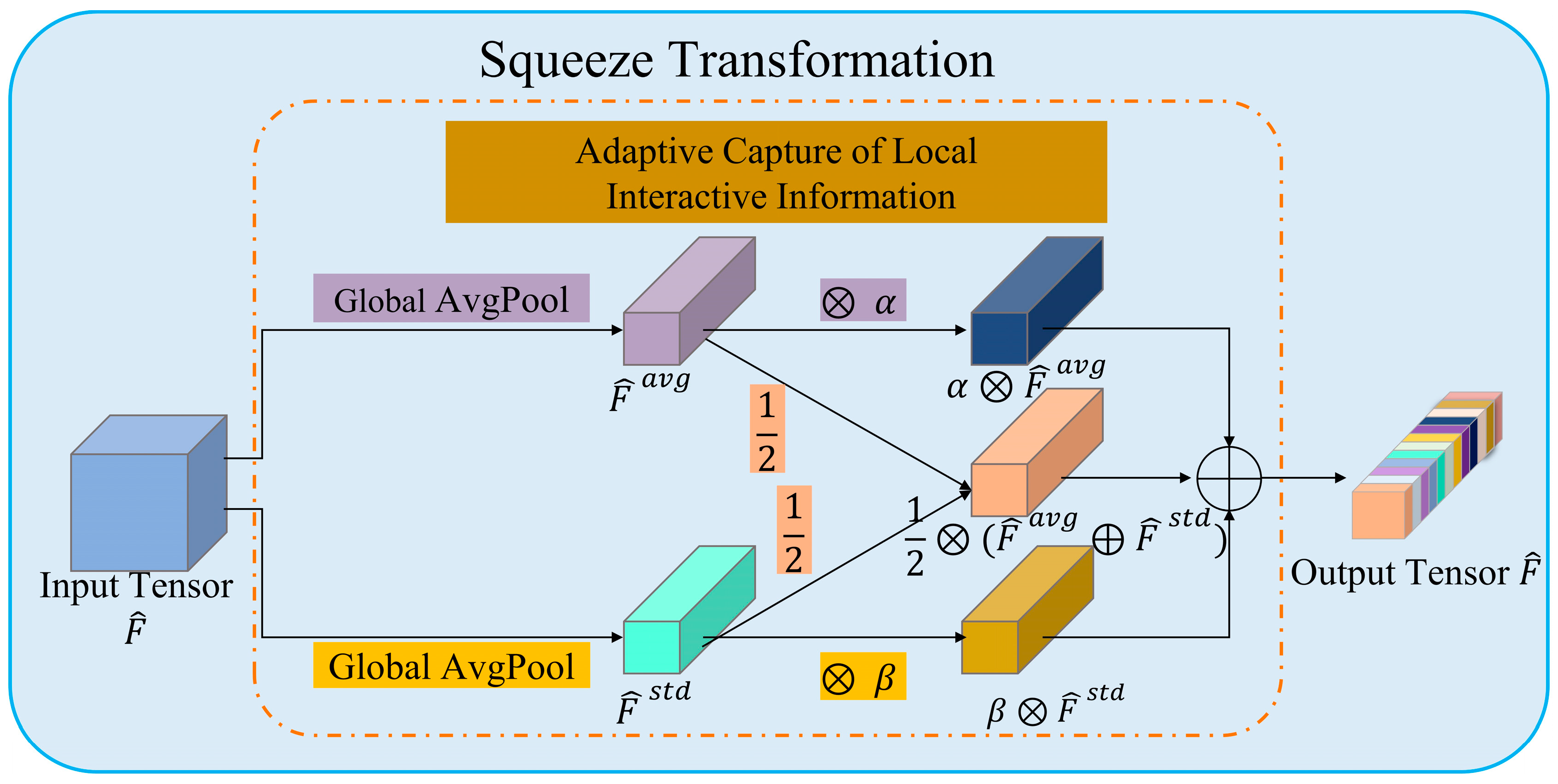
Squeeze: A method for adaptively combining dual interaction information

In the Squeeze module, effective interaction of features in the spatial and channel dimensions is achieved by combining mean pooling and standard deviation pooling [38]. High performance is maintained while the computational overhead is controlled. The process of the squeezing transformation is shown in Figure 8.

Figure 8 illustrates that the input $\stackrel{⏜}{\mathit{F}}$ is the spatial information of the feature map, which is combined of global average and standard deviation pooling. This process produces two distinct channel feature statistics, i.e., ${\stackrel{⏜}{\mathit{F}}}^{avg}$ and ${\stackrel{⏜}{\mathit{F}}}^{std}$, representing the average pooled and standard deviation pooled feature descriptors, respectively. More precisely, the two pooling processes for these channels can be represented individually in the following equations:

$${\stackrel{⏜}{f}}_m^{avg}=\frac{1}{H\times W}{\displaystyle \underset{i=1}{\overset{H}{\Sigma }}{\displaystyle \underset{j=1}{\overset{W}{\Sigma }}{\stackrel{⏜}{f}}_m}}\left(i,j\right)$$

(8)

$${\stackrel{⏜}{f}}_m^{std}=\sqrt{\frac{1}{H\times W}{\displaystyle \underset{i=1}{\overset{H}{\Sigma }}{\displaystyle \underset{j=1}{\overset{W}{\Sigma }}{\left({\stackrel{⏜}{f}}_m\left(i,j\right)-{\stackrel{⏜}{f}}_m^{avg}\right)}^2}}}$$

(9)

Among them, ${\stackrel{⏜}{f}}_m$ is the feature map of the $m\text{-}th$ channel for the input $\stackrel{⏜}{\mathit{F}}$, which is in the shape of 1 × H × W, where H and W refer to the height and width of the spatial feature map, respectively. $\stackrel{⏜}{\mathit{F}}\cdot {\stackrel{⏜}{f}}_m^{avg}$ and ${\stackrel{⏜}{f}}_m^{\mathit{std}}$ are used to distinct output feature descriptors, each associated with the $m\text{-}th$ channel. Subsequently, the inputs ${\stackrel{⏜}{\mathit{F}}}^{avg}$ and ${\stackrel{⏜}{\mathit{F}}}^{std}$ are sent to the adaptive combination mechanism to generate the channel feature descriptor $\widehat{\mathit{F}}$. This process can be expressed as:

$$\widehat{\mathit{F}}=T_{sq}\left(\stackrel{⏜}{\mathit{F}}\right)=\frac{1}{2}\otimes \left({\stackrel{⏜}{\mathit{F}}}_m^{avg}\oplus {\stackrel{⏜}{\mathit{F}}}_m^{std}\right)\oplus \alpha \otimes {\stackrel{⏜}{\mathit{F}}}_m^{avg}\oplus \beta \otimes {\stackrel{⏜}{\mathit{F}}}^{std}$$

(10)

The optimized trainable floating-point parameters α and β must have values between zero and one. Simultaneously, the input-dependent dynamics have the capacity to allocate varying weights to the mean pooled and standard deviation pooled features throughout different stages of image feature extraction. This promotes the distinctiveness of the output feature descriptors.

(2)

Motivation: A method for adaptively combining the capture of local feature interactions

The excitation transformation method is employed to capture the local interactions of features between channels, which are further transformed to maximize the usage of dimensionally relevant feature descriptors produced by the squeezing transform [38].

As shown in Figure 9, we can obtain the channel feature weight by taking the channel feature descriptor $\widehat{\mathit{F}}$ as an input via Equation (6). In this process, we only take the interaction with its $K_C$ neighbors for $m\text{-}th$ channel. The channel feature weight ${\tilde{f}}_m$ can be computed by the following equation:

$${\tilde{f}}_m={\displaystyle \underset{\xi =1}{\overset{K_C}{\Sigma }}{w}^{\xi }{\widehat{f}}_m^{\xi }},{\widehat{f}}_m^{\xi }\in {\Theta }_m^{K_C}$$

(11)

${\Theta }_m^{K_C}$ represents the collection of feature descriptors from $K_C$ adjacent channels connected to the initial $m\text{-}th$ channel, whereas $w^{\xi }$ represents the learnable parameters that are common and not unique to any one channel. The implementation of this transformation can be achieved by a 2D convolution technique using a kernel size of $\left(1,K_C\right)$, which can be expressed as:

$$C=\phi \left(K_C\right)=2^{\left(\lambda \times K_C+\gamma \right)}$$

(12)

Then, K_C can be approximately acquired if C is given.

$$K_C=\vartheta \left(c\right)={\left[\frac{{\log }_2\left(c\right)-1}{1.5}\right]}_{odd}$$

(13)

(3)

Integration: Triple focus collaboration

The augmented feature map ${\mathit{F}}^{″}$ can be refined in three branches represented as ${\mathit{F}}_W^{″}$, ${\mathit{F}}_H^{″}$, and ${\mathit{F}}_C^{″}$, respectively. This refinement process eventually produces the final refined feature map ${\mathit{F}}^{‴}$. It is achieved by a simple average summation in the integration stage with the following equation:

$${\mathit{F}}^{‴}=\frac{1}{3}\otimes \left(F_W^{″}\oplus F_H^{″}\oplus F_C^{″}\right)$$

(14)

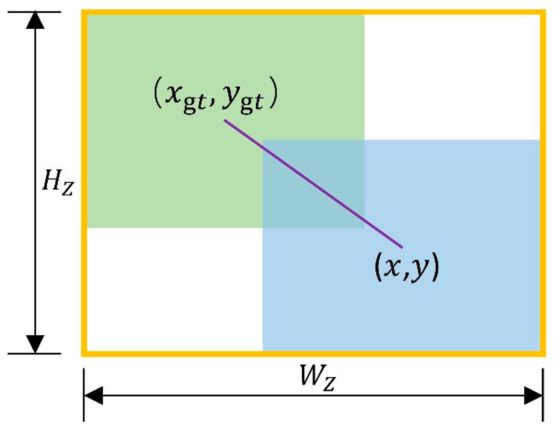
2.3.4. WIoUv3 Loss Function

During the training process of our newly designed Pine-YOLO model, it is crucial to utilize a bounding box loss function to guide the regression, and thus to reduce the bias between the predicted frame and the true frame, which increases the efficiency of the detection model. The loss function of YOLOv8 is described as:

$$L=L_{DFL}+L_{cls}+L_{box}$$

(15)

where $L_{DFL}$, $L_{cls}$, and $L_{box}$ represent the focal point loss, the class loss, and the bounding box regression loss, respectively.

The bounding box regression loss for YOLOv8 employs the CioU function with the following formula:

$$L_{\mathrm{CIOU}}=1-IoU+\frac{{\rho }^2\left(b,b^{gt}\right)}{c^2}+\alpha v$$

(16)

$$\alpha =\frac{v}{1-IoU+v}$$

(17)

$$v=\frac{4}{{\pi }^2}{\left(\arctan \frac{w^{gt}}{h^{gt}}-\arctan \frac{w}{h}\right)}^2$$

(18)

where $w^{gt}$, $h^{gt}$, $w$, and $h$ define the width and height of the real frame and the predicted frame, respectively. $\alpha$ refers to the weight function, v represents the similarity of the width-to-height ratio, and $IoU$ is the intersection ratio of the real frame and the predicted frame. $b^{gt}$ and b denote the central points of the boundaries of the real frame and the predicted frame, respectively. $\rho$ is the Euclidean distance between $b^{gt}$ and b. $c$ refers to the length of the diagonal of the smallest outer rectangle of the real frame and the predicted frame. $w^c$ and $h^c$ represent the dimensions of the smallest possible rectangle that can encompass both the real frame and the predicted frame, respectively.

$$c=\sqrt{{\left(w^c\right)}^2+{\left(h^c\right)}^2}$$

(19)

The CioU loss function has an obvious advantage over the traditional IoU in bounding box regression, which considers the variations in the geographical position, size, and shape of the predicted frame and the real frame. For instance, the distance of the bounding box regression, the centroid offset, the overlap area, and other factors make the bounding box regression converge better. However, from the formula calculating CioU in Equation (16), the parameter v only evaluates the similarity of the aspect ratio and does not accurately represent the actual relationship between the width and height of the real frame and the predicted frame. This would worsen the penalty for low-quality samples, weakening the generalization ability accordingly.

To address the disadvantages of CioU, we adopted WioUv3 (Wise-IoUv3) to deal with the loss function in this study, which incorporates a weighting coefficient to modify the correlation between each predicted frame and the real frame. It also considers the quality of the samples in relation to the CioU loss function. Additionally, it evaluates the standard of the anchor frames through a dynamic non-monotonic focusing mechanism [39]. WioUv3 is built upon the foundation of WioUv1. The formula to describe WioUv1 is presented below:

$$L_{WIoUv1}=R_{WIoU}{L}_{IoU}$$

(20)

$$R_{WIoU}=\exp \left(\frac{{\left(x-x_{gt}\right)}^2+{\left(y-y_{gt}\right)}^2}{{\left({W_g}^2+{H_g}^2\right)}^{\ast }}\right)$$

(21)

$$L_{IoU}=1-IoU$$

(22)

Here, $R_{WIoU}$ is the normalized length of the centroid connection representing the loss of a high-quality anchor frame. As shown in Figure 10, the blue and green rectangles represent the anchor frame and the target frame, respectively. $W_g$ and $H_g$ refer to the width and height of the smallest outer rectangle of the anchor frame and the target frame, respectively. $x$ and $y$ represent the coordinates of the centroid of the anchor frame, respectively, while $x_{gt}$ and $y_{gt}$ are the coordinates of the centroid of the target frame, respectively.

WioUv3 introduces a gradient gain distribution method to reduce the influence of harmful gradients as compared to WioUv1. This ensures the effect of high-quality anchor frames and strengthens the generalizability of the Pine-YOLO model. The WioUv3 formulas are:

$$L_{WIoUv3}=r\times L_{WIoUv1}$$

(23)

$$r=\frac{\beta }{\delta {\alpha }^{\beta -\delta }}$$

(24)

$$\beta =\frac{{L^{\ast }}_{IoU}}{\overline{L_{IoU}}}\in \left[0,+\infty \right]$$

(25)

where $\beta$ refers to the measured quality of the anchor frame by considering the presence of outliers, for which a smaller outlier suggests a better anchor frame. $r$ is a non-monotonic focusing factor that successfully mitigates the occurrence of bigger damaging gradients caused by low-quality samples. ${L^{*}}_{IoU}$ is a monotonic focusing factor, while $\overline{L_{IoU}}$ is a sliding average of $L_{IoU}$ with the momentum equalling to m. $\alpha$ and $\delta$ are the hyper-parameters. When $\beta =\delta$, $r=1$. When $\beta$ is equal to the specific value of $C$, the anchor frame will have higher gradient gain.

$\beta$ follows the change of $L_{IoU}$, so the gradient gain of the anchor frame can be continuously adjusted. According to the current quality of the anchor frame, the loss function can dynamically adjust the gradient gain allocation strategy.

2.4. Parameter Settings and Evaluation Metrics

With our newly designed Pine-YOLO, we carried out series of detection on pine wilt disease using our UAV images collected from Weihai. The experiments are performed with the NVIDIA GeForce RTX 3060 GPU and the Windows 10 operating system. PyTorch is employed for the deep learning framework. An automatic optimizer is employed with the following parameters: an initial learning rate of 0.01, a learning rate decay factor of 0.01, a batch size of 16, a momentum value of 0.937, a weight decay coefficient of 0.0005, a non-maximum suppression threshold of 0.5, a patience value of 50, and a pre-trained YOLOv8 model.

The employed assessment measures for the detection and classification outcomes are [email protected], [email protected]:0.95, Precision, Recall, and F1-score. The formulas to calculate these metrics are given below:

$$Precision=\frac{TP}{TP+FP}\times 100\%$$

(26)

Precision denotes the probability that the prediction target is correct. TP means that a diseased tree is correctly detected. FP means that a healthy pine tree is detected as diseased.

$$Recall=\frac{TP}{TP+FN}\times 100\%$$

(27)

Recall denotes the probability of a diseased pine tree being truthfully predicted. FN means that the diseased tree is incorrectly predicted to be healthy.

$$mAP=\frac{{\displaystyle \underset{n}{\overset{i=1}{\Sigma }}{A}_{i}P}}{n}$$

(28)

mAP represents the Precision accuracy of the detection process. [email protected] represents the average Precision at an intersection over the IoU criterion of 0.5. [email protected]:0.95 refers to the average mAP value with IoU from 0.5 to 0.95 with a step size of 0.05.

$$F1=\frac{2Precision*Recall}{Precision+Recall}\times 100\%$$

(29)

F1-score provides a consistent metric to measure the balance between Precision and Recall.

3. Results and Discussions

3.1. Detection Results from Alternative Methods

Figure 11a shows five images containing diseased trees and disease annotations in the testing dataset, and each image is taken under different conditions, such as different lighting and shading conditions. These various conditions directly affect the brightness and contrast of the images, and may mask or emphasize certain features of the pine trees, thus affecting the recognition results. In addition, the diversity of ground conditions, such as bare soil, grass, rocks, and other surface features, may also interfere with the target detection of pine trees. Particularly, in cases where the ground color is similar to that of a diseased pine tree, it is difficult for the detection algorithm to distinguish the pine tree from the background. At the same time, the presence of other background factors, such as vegetation, may confuse pine trees with the background, further increasing the likelihood of detection errors.

To address these problems, we performed detection by our newly designed Pine-YOLO model, and show the detection results in Figure 11d.

Table 1. Detection results obtained from different deep learning algorithms.

Detection Models	[email protected]	[email protected]:0.95	Precision	Recall	F1-Score
Faster-RCNN	76.00%	38.50%	68.42%	79.59%	73.58%
RetinaNet	70.80%	38.60%	67.80%	81.63%	74.08%
YOLOv5	82.72%	47.16%	68.81%	82.84%	74.76%
YOLOX	73.10%	46.40%	77.08%	75.51%	76.29%
DETR	81.92%	45.00%	80.39%	83.67%	82.00%
MA-Unet *	-	-	57.45%	50.56%	46.78%
YOLOv5-PWD *	84.5%	-	87.8%	76.8%	81.93%
Pine-YOLO	90.69%	49.72%	91.31%	85.72%	88.43%

The symbol “*” denotes that the model and its data are sourced from other references in the same research field.

summarizes the quantitative detection results of Pine-YOLO methods applied to testing images. We can find that the Pine-YOLO model exhibits exceptional performance, particularly in terms of [email protected] (90.69%) and Precision (91.31%). This demonstrates its high reliability in locating and predicting pine trees accurately. Pine-YOLO also presents a notable Recall of 85.72%, indicating its effectiveness in identifying the most diseased pine trees. As an average of Precision and Recall, F1-score reaches a relative high value of 88.43%, further confirming the superiority of Pine-YOLO in striking a balance between detection accuracy and coverage.

To make a clear comparison between our results and other deep learning algorithms, we also carried out detections using Faster R-CNN, RetinaNet, YOLOv5, YOLOX, and DETR, respectively. The detection results for all these algorithms are also listed in Table 1, Figure 12, and Figure S1 in Supplementary Materials. We can see from these data that the other algorithms also exhibit good performances in some metrics, for example YOLOv5 provides a relatively high [email protected] of 82.72%. However, as a whole, they showed a considerable number of missed detections and false detections, resulting in the low evaluation parameters. Moreover, Pine-YOLO also demonstrated superior performance in the more stringent metric of [email protected]:0.95 (49.72%), indicating its higher efficiency across different IoU thresholds. That is, Pine-YOLO demonstrated an overall superior ability to identify diseased pine trees correctly, confirming the strong accuracy and robustness of this model under varying lighting conditions.

To further validate our research findings, we compared the performance of Pine-YOLO with other previous methods mentioned in the literature within the same field, MA-Unet [40] and YOLOv5-PWD [41]. The data presented in the Table 1 clearly illustrate that Pine-YOLO in this work surpasses both MA-Unet and YOLOv5-PWD in terms of precision and recall, thereby also exhibiting a marked superiority in the F1 score. This comparison showcases the outstanding performance of Pine-YOLO in accurately identifying and classifying diseased pine trees.

3.2. Ablation Experiment

In this study, we introduced DSConv, MCA, and WIoUv3 into the YOLOv8 network to form the Pine-YOLO model. DSConv enhances the perception of the fine tubular structure of discolored pine branches by adaptively focusing on the fragile and curved local features of the tubular structure. MCA helps the model better understand the spatial properties of the pine trees and their representation in the image. It strengthens the attention of the model to the specific features of pine trees, and thus improves recognition accuracy and the generalization ability of the model for diseased pine tree recognition in variable natural environments. WIoUv3 uses a dynamic non-monotonic focusing mechanism (FM) to make the most realistic gradient gain allocation decision at each moment based on the current situation, improving the overall recognition accuracy and robustness.

The quantitative findings of ablation experiments are presented in

Table 2. Detection results obtained from quantitative ablation experiments. YOLOv8 serves as the benchmark network.

DSConv.	MCA	WIoUv3	[email protected]	[email protected]:0.95	Precision	Recall	F1-Score
-	-	-	78.46%	47.55%	74.42%	83.67%	78.77%
√	-	-	85.34%	43.11%	88.74%	83.67%	86.13%
-	√	-	85.56%	47.17%	82.90%	85.71%	84.28%
-	-	√	82.65%	50.61%	75.71%	82.64%	79.02%
√	√	-	88.70%	48.91%	93.64%	83.67%	88.37%
√	-	√	86.56%	49.06%	85.94%	87.64%	86.78%
-	√	√	87.76%	46.99%	89.82%	85.71%	87.72%
√	√	√	90.69%	49.72%	91.31%	85.72%	88.43%

The symbol “√” denotes the inclusion of a module or classification network in the baseline network, whereas the symbol “-“ signifies its absence.

. All models used on the testing dataset show significant performance improvements. The implementation of DSConv increases the [email protected] from 78.46% to 85.34%. This substantial enhancement indicates that DSConv can augment the Precision effectively in locating pine trees. The introduction of the MCA module independently boosts the Recall to 85.71%, underscoring its crucial role in capturing pine tree features. WIoUv3 achieves a competitive edge under the more comprehensive [email protected]:0.95 evaluation parameter with mAP reaching 50.61%, demonstrating a robust capability. When these three components are integrated into the YOLOv8 network to construct the Pine-YOLO model, it achieves the best detection results, which are shown in Table 2 and Figure 12 in detail. The data in Table 2 show that Pine-YOLO attains peak performance across all key metrics, especially achieving a high [email protected] of 90.69% and an F1-score of 88.43%, which verifies the significant superiority of DSConv, MCA, and WIoUv3 synergy in detection of pine wilt disease. In Figure 12, all types of algorithm combination do not show any missed detection in the testing images, while the false detection still remains. With the successive addition of these modules, the false detection rate gradually decreases. These phenomena prove that the newly designed Pine-YOLO model can extract the target features effectively and thus significantly improves recognition accuracy and reliability. Specifically, with the combined application of different modules in the Pine-YOLO algorithm, the superposition effect enables the model to distinguish the target from the background more accurately when it encounters complex image content. That is, in scenes with complex or similar features, Pine-YOLO effectively reduces false recognition and ensures highly accurate target detection. Additional ablation experimental results are included in Figure S2 in Supplementary Materials.

3.3. Pine-YOLO Composite Indicator Assessment and Discussion

The validation losses of Pine-YOLO, which are depicted in Figure 13a, are also analyzed thoroughly in this study. The gradual decrease in different loss metrics highlights the progress in learning how to identify pine trees more accurately. A significant decrease in Validation Box Loss is found in Figure 13a, which reveals the increasing accuracy in locating the bounding box of a diseased pine tree, which is critical for fine-tuning target detection in complex images. The continued decrease in Validation Class Loss in Figure 13a indicates the increased accuracy of Pine-YOLO in identifying the class of the targeted pine tree. In addition, the decrease in Validation Distribution-Focused Loss (DFL) further confirms the continued efforts of Pine-YOLO to improve localization details, particularly for accuracy on the edge of pine trees. As a consequence, these results demonstrate the effectiveness of the design and training strategy for Pine-YOLO in improving the accuracy of diseased pine tree detection results. Meanwhile, when the Pine-YOLO model deals with new and different data, it shows a smooth Validation Loss curve, indicating better consistency, reliability, and thus the generalization of this newly designed model.

The convergence curves of the performance metrics for Pine-YOLO reveal the detection exhibition at each training stage, which are shown in Figure 13b. Although these values, e.g., the Precision, Recall, [email protected], and [email protected]:0.95, can reach a relatively high level, the volatility of the Precision and Recall values in this model reminds us that we need to balance the ability to recognize positive and negative samples during the training process.

Beyond the detailed analyses of the accuracy and detection performance improvements highlighted above, it is also noteworthy to mention the distinct advantage of the model in terms of size. In our specific experimental environment configuration, compared to the Pine-YOLO model optimized to a compact size of 6.7 Mb, standard YOLOv5 models typically require around 18.0 Mb. The enhanced versions of YOLOv5, exemplified by Zhang et al. [33] with YOLOv5s-CA and YOLOv5s-ECA, showcase model sizes of 16.0 Mb and 14.4 Mb, respectively. These models demonstrate valuable improvements in detection accuracy through the integration of advanced attention mechanisms. This compact size of Pine-YOLO not only eases deployment but also indirectly boosts operational efficiency and processing speed, vital for real-time applications on resource-constrained platforms. Future research efforts can focus on more effective picture pre-processing techniques and refine the model structure to enhance the robustness and Precision of the model across various contexts.

4. Conclusions

In this paper, we incorporated DSConv, MCA, and WIoUv3 into a YOLOv8 network to construct a newly designed Pine-YOLO model for pine wilt disease detection. We utilized images exclusively captured in Weihai City to construct a dataset via a sliding window method, among which all diseased pine tree samples were individually labeled and verified on-site. Then, we used this dataset to train and test the detection performance of Pine-YOLOv8. The results show that the F1-score of this model is 88.43%, which is 14.85%, 14.35%, 13.67%, 12.14%, and 6.43% higher than that of Faster-RCNN, RetinaNet, YOLOv5, YOLOX, and DETR, respectively, suggesting excellent performance of our detection model. We also performed the ablation experiment to analyze the exact interactions of each new modules we introduced into the Pine-YOLO model. DSConv enhances the perception of geometrical structures by adaptively focusing on the fragile and curved local features of tubular structures in diseased pine tree branches. MCA strengthens the model’s attention to pine tree-specific features in complex and changing natural environments. This mechanism efficiently captures feature interdependencies between spatial dimensions and channels through parallel branching structures. Moreover, the squeezing transform adaptively aggregates bi-dimensional feature responses, alongside an excitation transform that adaptively captures local feature interactions, allowing for fine-tuning of the input feature map. WIoUv3 focuses on the common quality anchor frames and promote the overall recognition accuracy and robustness of the detector. Therefore, the newly designed Pine-YOLO model overcomes some disadvantages of normal deep learning algorithms in the field of pine wilt disease detection. Hence, it can be used by forestry managers for rapid detection of pine wilt disease, which helps to maintain the health and stability of the ecological environment.

References

1. Li, M.; Li, H.; Ding, X.; Wang, L.; Wang, X.; Chen, F. The detection of pine wilt disease: A literature review. Int. J. Mol. Sci. 2022, 23, 10797. [Google Scholar] [CrossRef]
2. Lu, X.; Huang, J.; Li, X.; Fang, G.; Liu, D. The interaction of environmental factors increases the risk of spatiotemporal transmission of pine wilt disease. Ecol. Indic. 2021, 133, 108394. [Google Scholar] [CrossRef]
3. Kim, B.-N.; Kim, J.H.; Ahn, J.-Y.; Kim, S.; Cho, B.-K.; Kim, Y.-H.; Min, J. A short review of the pinewood nematode, Bursaphelenchus xylophilus. Toxicol. Environ. Health Sci. 2020, 12, 297–304. [Google Scholar] [CrossRef]
4. Hao, Z.; Huang, J.; Li, X.; Sun, H.; Fang, G. A multi-point aggregation trend of the outbreak of pine wilt disease in China over the past 20 years. For. Ecol. Manag. 2022, 505, 119890. [Google Scholar] [CrossRef]
5. Gao, R.; Liu, L.; Li, R.; Fan, S.; Dong, J.; Zhao, L. Predicting potential distributions of Monochamus saltuarius, a novel insect vector of pine wilt disease in China. Front. For. Glob. Chang. 2023, 6, 1243996. [Google Scholar] [CrossRef]
6. Wang, W.; Zhu, Q.; He, G.; Liu, X.; Peng, W.; Cai, Y. Impacts of climate change on pine wilt disease outbreaks and associated carbon stock losses. Agric. For. Meteorol. 2023, 334, 109426. [Google Scholar] [CrossRef]
7. Sharma, A.; Cory, B.; McKeithen, J.; Frazier, J. Structural diversity of the longleaf pine ecosystem. For. Ecol. Manag. 2020, 462, 117987. [Google Scholar] [CrossRef]
8. Hu, G.; Yao, P.; Wan, M.; Bao, W.; Zeng, W. Detection and classification of diseased pine trees with different levels of severity from UAV remote sensing images. Ecol. Inf. 2022, 72, 101844. [Google Scholar] [CrossRef]
9. Zhang, C.; Kovacs, J.M. The application of small unmanned aerial systems for precision agriculture: A review. Precis. Agric. 2012, 13, 693–712. [Google Scholar] [CrossRef]
10. Guimarães, N.; Pádua, L.; Marques, P.; Silva, N.; Peres, E.; Sousa, J.J. Forestry remote sensing from unmanned aerial vehicles: A review focusing on the data, processing and potentialities. Remote Sens. 2020, 12, 1046. [Google Scholar] [CrossRef]
11. Syifa, M.; Park, S.-J.; Lee, C.-W. Detection of the pine wilt disease tree candidates for drone remote sensing using artificial intelligence techniques. Engineering 2020, 6, 919–926. [Google Scholar] [CrossRef]
12. Oide, A.H.; Nagasaka, Y.; Tanaka, K. Performance of machine learning algorithms for detecting pine wilt disease infection using visible color imagery by UAV remote sensing. Remote Sens. Appl. Soc. Environ. 2022, 28, 100869. [Google Scholar] [CrossRef]
13. Iordache, M.-D.; Mantas, V.; Baltazar, E.; Pauly, K.; Lewyckyj, N. A machine learning approach to detecting pine wilt disease using airborne spectral imagery. Remote Sens. 2020, 12, 2280. [Google Scholar] [CrossRef]
14. Yu, R.; Luo, Y.; Zhou, Q.; Zhang, X.; Wu, D.; Ren, L. A machine learning algorithm to detect pine wilt disease using UAV-based hyperspectral imagery and LiDAR data at the tree level. Int. J. Appl. Earth Obs. Geoinf. 2021, 101, 102363. [Google Scholar] [CrossRef]
15. Wu, D.; Yu, L.; Yu, R.; Zhou, Q.; Li, J.; Zhang, X.; Ren, L.; Luo, Y. Detection of the monitoring window for pine wilt disease using multi-temporal UAV-based multispectral imagery and machine learning algorithms. Remote Sens. 2023, 15, 444. [Google Scholar] [CrossRef]
16. Park, H.G.; Yun, J.P.; Kim, M.Y.; Jeong, S.H. Multichannel object detection for detecting suspected trees with pine wilt disease using multispectral drone imagery. IEEE J. Sel. Top. Appl. Earth Obs. Remote Sens. 2021, 14, 8350–8358. [Google Scholar] [CrossRef]
17. Li, W.; An, B.; Kong, Y. Data Augmentation Method on Pine Wilt Disease Recognition. In Proceedings of the Intelligence Science IV, 5th IFIP TC International Conference, Xi’an, China, 28–31 October 2022; pp. 458–465. [Google Scholar] [CrossRef]
18. Rao, D.; Zhang, D.; Lu, H.; Yang, Y.; Qiu, Y.; Ding, M.; Yu, X. Deep learning combined with Balance Mixup for the detection of pine wilt disease using multispectral imagery. Comput. Electron. Agric. 2023, 208, 107778. [Google Scholar] [CrossRef]
19. Cai, P.; Chen, G.; Yang, H.; Li, X.; Zhu, K.; Wang, T.; Liao, P.; Han, M.; Gong, Y.; Wang, Q.; et al. Detecting individual plants infected with pine wilt disease using drones and satellite imagery: A case study in Xianning, China. Remote Sens. 2023, 15, 2671. [Google Scholar] [CrossRef]
20. Zhang, R.; You, J.; Lee, J. Detecting pine trees damaged by wilt disease using deep learning techniques applied to multi-spectral images. IEEE Access 2022, 10, 39108–39118. [Google Scholar] [CrossRef]
21. Xia, L.; Zhang, R.; Chen, L.; Li, L.; Yi, T.; Wen, Y.; Ding, C.; Xie, C. Evaluation of deep learning segmentation models for detection of pine wilt disease in unmanned aerial vehicle images. Remote Sens. 2021, 13, 3594. [Google Scholar] [CrossRef]
22. Wang, J.; Zhao, J.; Sun, H.; Lu, X.; Huang, J.; Wang, S.; Fang, G. Satellite remote sensing identification of discolored standing trees for pine wilt disease based on semi-supervised deep learning. Remote Sens. 2022, 14, 5936. [Google Scholar] [CrossRef]
23. Chen, Y.; Yan, E.; Jiang, J.; Zhang, G.; Mo, D. An efficient approach to monitoring pine wilt disease severity based on random sampling plots and UAV imagery. Ecol. Indic. 2023, 156, 111215. [Google Scholar] [CrossRef]
24. Sun, Z.; Ibrayim, M.; Hamdulla, A. Detection of pine wilt nematode from drone images using UAV. Sensors 2022, 22, 4704. [Google Scholar] [CrossRef] [PubMed]
25. Hu, G.; Yin, C.; Wan, M.; Zhang, Y.; Fang, Y. Recognition of diseased Pinus trees in UAV images using deep learning and AdaBoost classifier. Biosyst. Eng. 2020, 194, 138–151. [Google Scholar] [CrossRef]
26. Qin, B.; Sun, F.; Shen, W.; Dong, B.; Ma, S.; Huo, X.; Lan, P. Deep learning-based pine nematode trees’ identification using multispectral and visible UAV imagery. Drones 2023, 7, 183. [Google Scholar] [CrossRef]
27. Huang, J.; Lu, X.; Chen, L.; Sun, H.; Wang, S.; Fang, G. Accurate identification of pine wood nematode disease with a deep convolution neural network. Remote Sens. 2022, 14, 913. [Google Scholar] [CrossRef]
28. Wu, K.; Zhang, J.; Yin, X.; Wen, S.; Lan, Y. An improved YOLO model for detecting trees suffering from pine wilt disease at different stages of infection. Remote Sens. Lett. 2023, 14, 114–123. [Google Scholar] [CrossRef]
29. Deng, X.; Tong, Z.; Lan, Y.; Huang, Z. Detection and location of dead trees with pine wilt disease based on deep learning and UAV remote sensing. AgriEngineering 2020, 2, 294–307. [Google Scholar] [CrossRef]
30. Li, F.; Liu, Z.; Shen, W.; Wang, Y.; Wang, Y.; Ge, C.; Sun, F.; Lan, P. A remote sensing and airborne edge-computing based detection system for pine wilt disease. IEEE Access 2021, 9, 66346–66360. [Google Scholar] [CrossRef]
31. Abdollahnejad, A.; Panagiotidis, D.; Surový, P.; Modlinger, R. Investigating the correlation between multisource remote sensing data for predicting potential spread of Ips typographus L. spots in healthy trees. Remote Sens. 2021, 13, 4953. [Google Scholar] [CrossRef]
32. Ren, D.; Peng, Y.; Sun, H.; Yu, M.; Yu, J.; Liu, Z. A global multi-scale channel adaptation network for pine wilt disease tree detection on UAV imagery by circle sampling. Drones 2022, 6, 353. [Google Scholar] [CrossRef]
33. Zhang, P.; Wang, Z.; Rao, Y.; Zheng, J.; Zhang, N.; Wang, D.; Zhu, J.; Fang, Y.; Gao, X. Identification of pine wilt disease infected wood using UAV RGB imagery and improved YOLOv5 models integrated with attention mechanisms. Forests 2023, 14, 588. [Google Scholar] [CrossRef]
34. Qin, J.; Wang, B.; Wu, Y.; Lu, Q.; Zhu, H. Identifying pine wood nematode disease using UAV images and deep learning algorithms. Remote Sens. 2021, 13, 162. [Google Scholar] [CrossRef]
35. Han, Z.; Hu, W.; Peng, S.; Lin, H.; Zhang, J.; Zhou, J.; Wang, P.; Dian, Y. Detection of standing dead trees after pine wilt disease outbreak with airborne remote sensing imagery by multi-scale spatial attention deep learning and Gaussian kernel approach. Remote Sens. 2022, 14, 3075. [Google Scholar] [CrossRef]
36. Li, Y.; Fan, Q.; Huang, H.; Han, Z.; Gu, Q. A modified YOLOv8 detection network for UAV aerial image recognition. Drones 2023, 7, 304. [Google Scholar] [CrossRef]
37. Qi, Y.; He, Y.; Qi, X.; Zhang, Y.; Yang, G. Dynamic Snake Convolution based on Topological Geometric Constraints for Tubular Structure Segmentation. In Proceedings of the 2023 IEEE/CVF International Conference on Computer Vision (ICCV), Paris, France, 1–6 October 2023; pp. 6047–6056. [Google Scholar] [CrossRef]
38. Yu, Y.; Zhang, Y.; Cheng, Z.; Song, Z.; Tang, C. MCA: Multidimensional collaborative attention in deep convolutional neural networks for image recognition. Eng. Appl. Artif. Intell. 2023, 126, 107079. [Google Scholar] [CrossRef]
39. Tong, Z.; Chen, Y.; Xu, Z.; Yu, R. Wise-IoU: Bounding box regression loss with dynamic focusing mechanism. arXiv 2023, arXiv:2301.10051. [Google Scholar] [CrossRef]
40. Ye, W.; Lao, J.; Liu, Y.; Chang, C.-C.; Zhang, Z.; Li, H.; Zhou, H. Pine pest detection using remote sensing satellite images combined with a multi-scale attention-UNet model. Ecol. Inf. 2022, 72, 101906. [Google Scholar] [CrossRef]
41. Gong, H.; Ding, Y.; Li, D.; Wang, W.; Li, Z. Recognition of Pine Wood Affected by Pine Wilt Disease Based on YOLOv5. In Proceedings of the 2022 China Automation Congress (CAC), Xiamen, China, 25–27 November 2022; pp. 4753–4757. [Google Scholar] [CrossRef]
Figure 1. Detailed geographical location of the investigated area in this work with corresponding remote sensing images.
Forests 15 00737 g001
Figure 2. Schematic diagram of image cropping with (a) regular grid and (b) overlapping region, respectively.
Forests 15 00737 g002
Figure 3. Graphical representation of the mosaic data pre-processing technique integrated within the YOLOv8 model.
Forests 15 00737 g003
Figure 4. Diagram of the Pine-YOLO model.
Forests 15 00737 g004
Figure 5. Illustration of the dynamic snake convolution added into YOLOv8 model, which uses input feature maps to learn deformations and selectively emphasizes local aspects of elongated zigzags.
Forests 15 00737 g005
Figure 6. Illustration depicting (a) the coordinate calculation process of DSConv and (b) visualization of the receptive field of DSConv.
Forests 15 00737 g006
Figure 7. Schematic diagram of MCA module.
Forests 15 00737 g007
Figure 8. Illustration of the squeeze transform in the MCA module, using an adaptive mechanism for aggregating global mean and standard deviation information.
Forests 15 00737 g008
Figure 9. Illustration of the planned alteration of excitation in the MCA module.
Forests 15 00737 g009
Figure 10. Schematic diagram of the anchor frame and the target frame.
Forests 15 00737 g010
Figure 11. (a) Test images with labels. Detection results by (b) Faster-R CNN, (c) RetinaNet, and (d) Pine-YOLO algorithms. Among these images, the yellow, red, and blue rectangles represent true positives (TPs), false negatives (FNs), and false positives (FPs), respectively.
Forests 15 00737 g011
Figure 12. Ablation experiment results with (a) YOLOv8, (b) YOLOv8 + DSConv, (c) YOLOv8 + MCA, (d) YOLOv8 + WIoUv3, and (e) Pine-YOLO, respectively. Among these images, the yellow and blue rectangles represent true positives (TPs) and false positives (FPs), respectively.
Forests 15 00737 g012
Figure 13. Convergence curves of (a) Validation loss for Pine-YOLO model and (b) Performance metrics.
Forests 15 00737 g013