Unveiling the Influence of Climate and Technology on Forest Efficiency: Evidence from Chinese Provinces

Abstract

The objective of this study is to examine the impact of climate and technology on forest efficiency (FE) in China’s provinces from 2002 to 2020. First, the study used SBM-data envelopment analysis (SBM-DEA) to estimate Chinese provinces’ FE using multidimensional forest inputs and outputs. The climate influence is assessed using temperature, precipitation, sunlight hours, and carbon dioxide levels in the second phase. A climate index was created using principal component analysis (PCA) for a complete estimation. In addition to prior research, we analyze the technology impact through two technological indicators: (i) research and development, and (ii) investment in forests. Furthermore, we explore the non-linear influence of economic development on both FE and climate quality. The regression study by CupFM and CupBC found that temperature and precipitation increase FE, whereas sunlight hours and carbon emissions decrease it. The positive association observed between Climate Index1, and the negative relationship noted for Climate Index2, suggests that forests positively influence climate conditions, signifying that an improvement in FE leads to an improvement in climate quality. Technology boosts forest productivity and climatic quality. The environmental Kuznets curve shows an inverted U-shape relationship between economic development and FE. Similarly, climate and economic development have an inverted U-shaped EKC relationship. Urbanization reduces FE due to human growth and activity. Our findings are important for forest management, climate change, and sustainable development policymakers and scholars.

1. Introduction

There has not been enough attention on how climate factors and technology can make forest use more efficient. To address this knowledge void, the primary objective of this study is to analyze the impact of climate factors such as temperature, precipitation, sunlight hours, and CO₂ on China’s forest efficiency (FE). Simultaneously, the question naturally posits here: why is China positioned as a pivotal locus for research in this domain? Two compelling reasons underline the significance of China in this regard. Firstly, China is a major actor in the global forestry scene due to its vast forest cover, which extends throughout temperate, subtropical, and tropical zones [1,2]. With approximately 211 million hectares (Mha) of tree cover, China ranks fifth globally in terms of forested area. Secondly, China’s steadfast commitment to fostering sustainable forestry practices assumes paramount importance in the broader context of endeavors aimed at achieving carbon neutrality by 2060.

Recognizing the crucial role of forests in environmental conservation, China has undertaken extensive initiatives for forest restoration and afforestation. To increase its forest stock volume, since 2015, the Chinese government has committed considerably to its nationally determined contributions (NDCs) [3]. China has had a remarkable rise in forest coverage, going from 8.6% in 1949 to 23.04% by the end of 2020. The country’s large and diverse topography contains a substantial portion of the world’s forest resources. Much of this expansion is attributable to the fruitful reforestation campaigns of the 1960s and 1970s. The government is also working to improve forest sector risk management systems related to climate change.

The impact of climate on forests has great implications and influences their health, composition, and overall ecological dynamics [4]. For instance, changes in temperature, precipitation patterns, and intense weather events can affect forest ecosystems, disrupting the supply of plant and animal species and the overall biodiversity [5]. However, the effect of climate on FE is positive or negative depending on location and weather. For example, one primary climate factor is temperature, which affects FE in two ways. Temperature change can affect the growth and metabolism of trees and other plants [6]. Rising temperatures may lead to shifts in geographic distributions of certain species and the composition of forest growth. Furthermore, warmer temperatures may contribute to more efficient carbon sequestration, as enhanced tree growth can lead to greater carbon uptake and storage in forest ecosystems [7,8]. On the other hand, intense temperature can also negatively impact FE. High temperatures can disrupt the timing of seasonal events in forests and affect the synchronization of ecological interactions. The second important factor is the precipitation pattern, which can take the form of prolonged droughts or increased rainfall, and can impact plant water availability. Drought conditions lead to water stress, reduced growth, and increased susceptibility to pests and diseases [9]. According to Shi et al. (2016) [10], changes in precipitation patterns and rising temperatures may negatively impact the growing circumstances of many tree species. As a result, adjustments need to be made to planting and harvesting techniques.

Apart from that, carbon dioxide (CO₂) in the atmosphere can significantly impact forest ecosystems, influencing their efficiency, health, and overall functionality [11,12]. Rapid changes in CO₂ levels can be positive and negative, depending on various factors such as the concentration of atmospheric carbon dioxide, environmental conditions, and management practices. For instance, through the carbon fertilization effect, rising atmospheric CO₂ concentrations can drive photosynthetic activity in trees and other plant life, thereby increasing output [13]. Higher CO₂ levels allow plants to maintain photosynthesis while lowering water loss through stomatal control [14]. This can improve forest resistance to drought stress and resource efficiency in water-limited areas. However, increasing carbon emissions can disrupt forest ecosystem connections by interrupting their timing and altering the chemical composition of plant tissues. In summary, climate change, through temperature, sunlight hours, carbon, and precipitation pattern, poses challenges to FE by influencing species composition, disrupting natural regeneration processes, and increasing the vulnerability of forests to pests and diseases.

Many scholars have identified the various dynamic nexuses between FE and climate. For instance, Reyer et al. (2017) [15] examined how climate change affects forest productivity. Addas’s (2023) [16] study highlights the importance of forests in enhancing human well-being and addressing environmental issues such as air pollution. According to Torun and Altunel (2020) [17], windstorms pose a significant risk to Turkey’s woods. Boisvenue and Running (2006), García-Valdés et al. (2020), Pecchi et al. (2019), and Soucy et al. (2021) [18,19,20,21] are among the numerous researchers that have discovered the long-term effects of climate on forest growth. Forest carbon sink efficacy in 30 locations in China was also studied by Wei and Shen (2022) [22].

Along with that, technology has substantial potential to enhance forest resource management. Thus, the second objective is to analyze the role of technology in improving Chinese FE. The Chinese government has also implemented significant measures to expand forest cover further and optimize total factor productivity through sustainable forest management practices. Furthermore, China intends to utilize technological advancements, mechanization, and scientific research to enhance its forest resource efficiency and reduce environmental impacts [23]. According to Montoya et al. (2023) [24], technology gives forest administrators the ability to make knowledgeable judgments about the distribution of resources, the identification of wildfires, and the management of pests, all of which improve the general vitality of the forest. Li et al. (2017) [25] highlighted the critical need for China to increase investment in technology to enhance resource efficiency. Cheng et al. (2010) [26] looked at the flow properties of wood and wood byproducts throughout the early years of China’s economic development between 1953 and 2000. They emphasize increasing research and development efforts to promote innovation and limit the exploitation of resources. Wei and Shen (2022) [22] assessed the effectiveness of trees in absorbing carbon dioxide, emphasizing the need to improve the industry’s structure through scientific and technological advancements. Investing in human capital and incorporating technology should be top priorities for sustainable forestry operations [27]. Hence, the government must give priority to these issues to improve the effectiveness and long-term viability of forest management [28,29,30], which serves as the foundation for the subsequent assumptions. Improving efficiency in the forestry industry is essential for maintaining a balance between economic development and environmental sustainability. These activities boost economic growth and affect the forest’s sustainable use of resources, including carbon sequestration, biodiversity conservation, and timber availability [31]. Further, technology has substantial potential to enhance forest resource management as remote sensing, GIS, and satellite images are examples of cutting-edge technologies that could greatly improve forest resource management by providing current information on forest health, monitoring, and management [25,26].

The study’s objective is to evaluate the impact of climate and technology on FE of China provinces from 2002 to 2020. Simultaneously, the study captured the impact of FE on improving climate quality. According to our knowledge of the topic, we have not found a comprehensive study regarding climate factors and FE. Therefore, this study fills this gap in the existing research in the following way. First, the study measures the FE of the 30 Chinese provinces using inputs and outputs. Second, this study used various climate factors (temperature, precipitation, sunlight hours, and carbon dioxide) to assess the climate impact on FE. Third, the study used two technology indicators (high technology expenditure indicators and investments in forest technology). Fourth, the study incorporated the non-linear impact of economic development on FE and simultaneous climate quality. This makes this study a distinguishing addition to the literature. Based on the study objectives, this study revolves around the following five research questions:

• Do various climate factors such as temperature, precipitation, sunlight hours, and carbon dioxide levels influence forest efficiency?
• What is the combined impact of these climate factors on forest efficiency, and how can it be quantified using a climate index?
• How do technological advancements affect forest productivity and climatic quality?
• What is the relationship between economic development and forest efficiency, and does it follow the environmental Kuznets curve?
• How does urbanization influence forest efficiency considering human growth and activity?

2. Materials and Methods

This study analyzes the nexuses between climate factors, technology, and FE in China. This study utilized a sample of 30 Chinese provinces (

Table A1. List of provinces.

Zhejiang	Ningxia	Hebei
Yunnan	Liaoning	Hainan
Xinjiang	Jilin	Guizhou
Tianjin	Jiangxi	Guangxi
Sichuan	Jiangsu	Guangdong
Shanxi	Inner Mongolia	Gansu
Shanghai	Hunan	Fujian
Shandong	Hubei	Chongqing
Shaanxi	Henan	Beijing
Qinghai	Heilongjiang	Anhui

) from 2002 to 2020. The identification of a time frame depends on the presence of data.

Table 1. Descriptive Analysis of Variables.

Variable (s)	Acronyms	Data Unit (s)	Mean	Std.	Min	Max
Forest Efficiency	FE	Input variables: (i) Forest area (measured in 10,000 hectares), (ii) Investment (measured in 10,000 Yuan), (iii) Number of employees (measured in 10,000 persons).Output variable: (i) Forestry output value (measured in 100 million yuan).	0.528674	0.316123	0.0367	1
Temperature	Temp	Temp (°C)	14.80526	6.500424	1	113
Precipitation	Precp	Precp (millimeter)	973.6053	1057.641	75	22,111
Sunlight	SH	SH(Hours)	2083.616	1272.826	598	26,512
Carbon Emission	CO2	CO2 emissions (mt)	299.133	267.4526	1.009399	1924.954
Economic Development	GDP	GDP per capita (yuan)	38,037.18	27,576.64	3257	164,889.5
Technology1	Tech1	High-tech spending on scientific research activities	38,519.1	27,780.62	3257	164,889
Technology2	Tech2	Completed investment in forest (10,000)	827,440.9	1,291,055	3591	1.10 × 107
Urbanization	Urb	Urban population	52.23012	15.42139	20.85	90.26

displays a comprehensive summary of the variables and their corresponding descriptive statistics. Both the dependent and independent variable trends for 2020 are shown in Figure 1 and Figure 2, and are essential to our analysis.

2.1. Forest Efficiency (Dependent Variable)

Forest efficiency, the dependent variable, is measured through several inputs, including (i) forest area, (ii) investment, and (iii) number of employees. Output is measured by (i) forestry output value by data envelopment method (for formula, see Section 3).

2.2. Climate and Technology (Major Independent Variables)

2.2.1. Climate Indicators’ Index

The first primary independent factors are related to climate. When discussing climate, crucial elements such as temperature, precipitation, sunlight duration, and carbon dioxide emission are regarded as key aspects [32]. These climatic variables have a decisive impact on the environmental circumstances that directly and indirectly affect forest ecosystems. For instance, the development and health of trees are influenced by temperature and precipitation patterns. At the same time, the duration of sunlight hours is a basic activity for forest foliage. Furthermore, it is crucial to monitor carbon dioxide levels since it is a fundamental greenhouse gas that significantly impacts the global climate. The study intends to analyze climate-related variables and their impact on FE. It offers significant insights into the complex interaction between climatic elements and technology features in sustainable forest management. Simultaneously, the study highlights the importance of forests in climate quality. The study constructed the two-climate index using principal component analysis (PCA).

2.2.2. Calculation of Climate Index (Principal Component Analysis)

The current study utilized the PCA method, initially developed by Pearson (1901) [33] and subsequently enhanced by Hotelling (1933) [34], to construct a composite climate index. The study constructs two climate indices. Climate Index1 used three climate indicators: (i) temperature (temp (°C)), (ii) precipitation (millimetre), and (iii) sunlight (hours). These variables are commonly used to assess climate conditions.

Climate Index2 used four climate indicators: (i) temperature (temp (°C)), (ii) precipitation (millimetre), (iii) sunlight (hours), and carbon emission (mt). The addition of carbon dioxide emissions enhances Climate Index2 over Climate Index1. Climate Index2, which considers CO₂ emissions and traditional climatic parameters, may provide a more complete and comparative assessment of climate trends and their economic implications.

2.2.3. Technology Indicators

The productivity of forest management is greatly affected by technological advances [35]. Thus, the study included two technology indicators: (i) technological development-1 (Tech1) and (ii) technological development 2 (Tech2). The impact of Tech1 is measured through the high technology expenditure indicators, while the impact of Tech2 is assessed through investments in forest technology.

2.2.4. GDP and Urbanization Indicators

Consistent with Hao et al. (2019) [36], we utilized GDP per capita and squared GDP per capita as indicators of economic development at the provincial level. This analysis aims to assess the influence of the different developmental levels of Chinese provinces on forest and climate conditions. Furthermore, this analysis included the influence of urbanization as a controlled variable developed from previous research to reduce the possibility of biases caused by omitted factors. Therefore, the variable is included in the study based on the works of Liu et al. (2019) [37].

2.3. Empirical Modelling

In the previous section, we measured the climate indexes and the FE. However, these are not enough to empirically estimate the climate impact on FE. This study composed an empirical research model to examine the impact of climate, technology, economic growth, and urbanization on FE, which was considered the dependent variable. The basic framework of the baseline models is outlined as follows:

$${FE}_{it}=f({{CF}_{it}Tech}_{it},{GDP}_{it},{{GDP}^2}_{it},{Urb}_{it})$$

(1)

$${FE}_{it}=f({{CFindex}_{it}Tech}_{it},{GDP}_{it},{{GDP}^2}_{it}{Urb}_{it})$$

(2)

$${CFindex}_{it}=f({FE}_{it}{Tech}_{it},{GDP}_{it},{{GDP}^2}_{it}{Urb}_{it})$$

(3)

On the left-hand side, $FE$ is the forest efficiency of the Chinese province. $CF$ represents the four climate factors. While $CFIndex$is the climate indexes (i) $CFindex1$ indicates the Climate Index1, and (ii) $CFindex2$, is the Climate Index2. i is the cross-section of panels, and t represents time.

We enhance the empirical baseline models in the subsequent empirical models’ equations.

$$\mathrm{Model}-1:{FE}_{it}={\alpha }_0+{\alpha }_1{CF}_{it}+{\alpha }_2{Tech}_{it}+{\alpha }_3{GDP}_{it}+{\alpha }_4{{GDP}^2}_{it}+{\alpha }_5{Urb}_{it}+{\mu }_{it}$$

(4)

$CF$ Climate factors that are measured through temperature, precipitation, sunlight hours, and carbon dioxide emission, $Tech$ ($Tech1,\mathrm{a}\mathrm{n}\mathrm{d}Tech2)$, are the technological measurement, determined by expenditure on high technology and investment in the forest, $GDP$ is per capita economic development to measure the initial level of development, while ${GDP}^2$ measure the later economic development phase, $Urb$ is the urbanization of Chinese provinces.

$$\mathrm{Model}-2:{FE}_{it}={\alpha }_0+{\alpha }_1{CFindex}_{it}+{\alpha }_2{Tech}_{it}+{\alpha }_3{GDP}_{it}+{\alpha }_4{{GDP}^2}_{it}+{\alpha }_5{Urb}_{it}+{\mu }_{it}$$

(5)

$$\mathrm{Model}-3:{CFindex}_{it}={\alpha }_0+{\alpha }_1{FE}_{it}+{\alpha }_2{Tech}_{it}+{\alpha }_3{GDP}_{it}+{\alpha }_4{{GDP}^2}_{it}+{\alpha }_5{Urb}_{it}+{\mu }_{it}$$

(6)

In Model-2, $CFindex$ represents ($CFindex1$ and $CFindex2$), the climate indices measured through PCA. $CFindex1$ is measured using temperature, precipitation, and sunlight hours, while $CFindex2$ is measured using temperature, precipitation, sunlight hours, and carbon dioxide for comprehensive analysis.

3. Empirical Approaches

The current study analysis started by examining the variability in slopes due to cross-sectional dependence, and then analyzed unit roots and assessed co-integration. Finally, the long-term parameters of the variables under study are meticulously estimated.

• Step-1: SBM Data Envelopment (DEA) for FE.

Tone (2002) [38] introduced the non-radial Slacks-based measure (SBM) method for efficiency assessment in data envelopment analysis (DEA). SBM is practical as it immediately handles surplus inputs and insufficient outcomes. SBM evaluates efficiency nuancedly by considering slack (the variance between inputs and outputs at the production frontier). This approach function can be explained as:

Consider a hypothetical study comprising n decision-making units (DMUs) designated as “Provinces.” m input indicators and s output indicators define each DMU. Let $B_j$ Represent the $j$-th DMU, where j ranges from 1 to n. The input indicators of DMU $B_j$, denoted as $\left[x_{ij}\right]$, encompass a vector of dimension m × 1, where i varies from 1 to m. Similarly, the output indicators of DMU $B_j$, denoted as $\left[y_{rj}\right]$, consist of a vector of dimension $s\times 1$, where r ranges from 1 to $s$. The relative efficiency value of the j_0-th DMU is represented as $h_{j0}$. Subsequently, let us elucidate the operational mechanism of the output-oriented SBM-DEA model with variable returns to scale.

$$\begin{array}{c}\mathrm{Min}{h}_{j0}=\theta \\ \mathrm{s}.\mathrm{t}\left\{\begin{array}{l}{\displaystyle \sum _{j=1}^n}{\lambda }_j{x}_{ij}\le \theta x_{ij0},i=1,\dots ,m\\ {\displaystyle \sum _{j=1}^n}{\lambda }_j{y}_{rj}\ge y_{ij},r=1,\dots ,s\\ {\displaystyle \sum _{j=1}^n}{\lambda }_j=1,{\lambda }_j\ge 0,j=1,\dots ,n\end{array}\right.\end{array}$$

(7)

The efficiency value denoted as $\theta$ at the $j$-th position is determined by a non-negative vector ${\lambda }_j$. A DMU is classified as efficient exclusively when $\theta$ equals 1, signifying its operation at maximum efficiency. Conversely, a value of $\theta$ other than 1 indicates inefficiency, implying potential for enhancement in the DMU’s performance.

• Step-2: Cross-sectional dependence (CD) and Slope Heterogeneity (SH)

Subsequently, we utilized advanced econometric algorithms suitable for analyzing the suggested model’s Equations (4)–(6). The algorithms consider the consistency of gradients and the correlation between distinct groups’ cross-sections. Pesaran’s (2006) [39] research emphasized the importance of accounting for cross-sectional dependence in panel data analysis to prevent substantial bias and inaccuracies in estimated results. First, the data is checked for the presence of CD before calculating the elasticities of coefficients. Then, the uniformity of slopes across panels is examined. We employed the test CD developed by Pesaran (2004) [40]. Further, the study employed the Pesaran and Yamagata (2008) [32] slope homogeneity (SH) test for the absence of slope differences between panels.

• Step-3: Unit Root Checks

Testing time series data for unit roots is essential to avoid erroneous regression findings due to non-stationarity issues during model estimation [41]. The investigation commenced by examining the presence of unit roots and originally employed the Im et al. (2003) [42] integrated panel stationarity (IPS) test. This test allows for autoregressive (AR) parameter variations across all the cross-sections based on the Dickey-Fuller procedures. In addition, we conducted Pesaran’s (2007) [43] unit root test on each series, which takes into account the cross-sectional dependency to analyze the stationary characteristics of the series.

• Step-4: Co-integration Exploration

Unit root testing itself is insufficient for establishing the presence of co-integration among the series. This research utilized co-integration as a first step before calculating the elasticities of the coefficients [44]. Traditional first-generation co-integration tests may not be appropriate for panel data analysis if variables show cross-sectional connection, potentially leading to misleading results [45]. We used the Westerlund (2008) [46] method to detect co-integrating vectors in panel datasets. This strategy presents a dual-testing approach while also considering the potential negative effects of cross-sectional dependence. The test individually examines the extent of error correction for each group and the full panel. Westerlund utilized two distinct group-mean tests to examine the null hypothesis of no co-integration. The first group utilizes $Gt$ and $Ga$ statistics, while the second group depends on panel testing based on $Pt$ and $Pa$. This test yields impartial outcomes in the presence of serially correlated and heteroscedastic error factors. Furthermore, it considers the association between different sections and any interruptions in the data [46].

• Step-5: Long-run Parameter Estimations

Although many econometric methods for estimating parameter elasticities are available in the literature, the best course of action is to narrow down the econometric method options according to properties of the data. While the approach adapts to the specifics of the selected data dimension, researchers should be free to select an estimator that best suits their needs after carefully considering the data’s benefits and drawbacks. Following, this study used the “Continuously Updated and Fully Modified (CupFM)” and “Continuously Updated and Bias Corrected (CupBC)” estimators developed by Bai and Kao (2006) [47].

We may obtain the continuously updated (CuP) estimator by iterating on these two models.

$$\widehat{b}=({\sum }_{i=1}^k\acute{x_i}{m}_{\widehat{f}}{x}_i{)}^{-1}{\sum }_{i=1}^k\acute{x_i}{m}_{\widehat{f}}{e}_i$$

(8)

$$\widehat{{fv}_{nt}}=\left[\right({nt}^2{)}^{-1}{\sum }_{i=1}^k(e_i-x_i\widehat{b}\left)\right(e_i-x_i\widehat{b}\acute{)}]\widehat{f}$$

(9)

Here, $m_{\widehat{f}}=i_t-t^{-2}\widehat{f}\widehat{\acute{f}},i_r=t^{-2}\acute{\widehat{f}}\widehat{f},v_{nt}$ represents a decreasing diagonal matrix of r maximum eigenvalues. So, Bai et al. (2009) [48] presented the Cup Fully Modified and Cup Bias Corrected estimators, which are fully adjusted to reduce bias. The CupFM estimator is obtained by solving the following two equations successively.

$$CupFM={\left[{\displaystyle \sum _{i=1}^k{x^{\prime }}_i{m}_{\stackrel{⌢}{f}}{x}_i}\right]}^{-1}{\displaystyle \sum _{i=1}^k\left[{x^{\prime }}_i{m}_{\stackrel{⌢}{f}}{e^{+}}_i-t[{\stackrel{⌢}{\overline{\Delta }}}_{eui}^{+}-{\stackrel{⌢}{\overline{\phi }}}_i{\stackrel{⌢}{\overline{\Delta }}}_{nu}^{+}]\right]}$$

(10)

$$\stackrel{⌢}{f}{v}_{nt}=\left[{(n{t}^2)}^{-1}\right]{\displaystyle \sum _{i=1}^n(e_i-x_i{\stackrel{⌢}{b}}_{CupFM}})(e_i-x_i{\stackrel{⌢}{b}}_{CupFM}{)}^{\prime }\stackrel{⌢}{f}$$

(11)

where $e_{it}^{+}=e_{it}+{\mathsf{\Omega }}_{ubi}{\mathsf{\Omega }}_{bi}^{-}(\begin{array}{c}\mathsf{\Delta }{x}_{it}\\ \mathsf{\Delta }{f}_t\end{array})$. Whereas the CupBC proposed by Bai et al. (2009) [48] can be approximated with, ${\stackrel{⌢}{b}}_{CupBC}=b_{Cup}-t^{-1}{\stackrel{⌢}{\varphi }}_{nt}$, where ${\stackrel{⌢}{\varphi }}_{nt}={\left\{{(n{t}^2)}^{-1}{\displaystyle \sum _{i=1}^k{\stackrel{⌢}{z}}_i^{/}{\stackrel{⌢}{z}}_i}\right\}}^{-1}[n^{-1}{\displaystyle \sum _{i=1}^k{\stackrel{⌢}{\phi }}_i]}$ is the estimator of the bias term. Their associated covariances ${\stackrel{⌢}{\overline{\mathsf{\Omega }}}}_i={\displaystyle \sum _{T=t+1}^{t-1}\mathsf{{\rm Y}}\left[\frac{i}{k}\right]}{\stackrel{⌢}{\overline{\mathsf{\Psi }}}}_{\rho }[i]$ and long-term covariance matrix ${\stackrel{⌢}{\overline{\mathsf{\Delta }}}}_i={\displaystyle \sum _{i=0}^{t-1}\mathsf{{\rm Y}}}\left[\frac{i}{k}\right]{\stackrel{⌢}{\overline{\mathsf{\Psi }}}}_{\rho }[i]$ are calculated. CupFM and CupBC are distributed according to a normal distribution, allowing for typical conclusions to be made.

This method offers significant benefits compared to similar methods. The CupFM and CupBC estimators surpass traditional econometric methods by properly handling cross-sectional dependence, endogeneity, and autocorrelation concerns. They consistently produce dependable outcomes when used with panel datasets. These estimators perform well in various analytical situations, especially in producing reliable and thorough estimates of the external features of regressors while ensuring efficiency for all integration orders except for higher-order integrated series (I(2) or higher). Despite endogeneity, these estimators give positive outcomes [48]. We utilized CupFM and CupBC estimators because of their advantages in this investigation. The study utilized the fully modified OLS method to guarantee the precision and dependability of the results.

4. Results and Discussion

4.1. Findings of Data Envelopment Analysis for Forest Efficiency

Figure 3 displays the FE values measured by the SBM-DEA method for the provinces of China between 2002 and 2020. FE is a metric that assesses how a province utilizes its forest resources, with a higher FE value signifying a greater degree of efficiency. The province of Anhui shows the consistently highest FE. Similarly, Fujian, Guangdong, and Guangxi also demonstrate high levels of FE over the years, suggesting effective usage of their forest resources. Chongqing FE is continuously increasing.

Xinjiang shows lower rankings in FE, indicating possible issues or inequities in managing forest resources. The study shows the different ways that China’s forest resources have been used wisely in different parts of the country over the last 20 years. Figure 4 shows the average FE of different regions, with southern and eastern China having the highest average efficiency and Northwest China and Northern China having the lowest FE.

4.2. Findings of Climate Indices’ Principal Component Analysis

Table 2. PCA of Climate Index1.

Component	Eigenvalue	Difference	Proportion	Cumulative
Comp1	1.47419	0.633417	0.4914	0.4914
Comp2	0.840774	0.15574	0.2803	0.7717
Comp3	0.685034	.	0.2283	1
Variable (s)	Comp1	Comp2	Comp3
Temperature	0.628	0.1557	0.7625
Precipitation	0.5811	0.5579	−0.5925
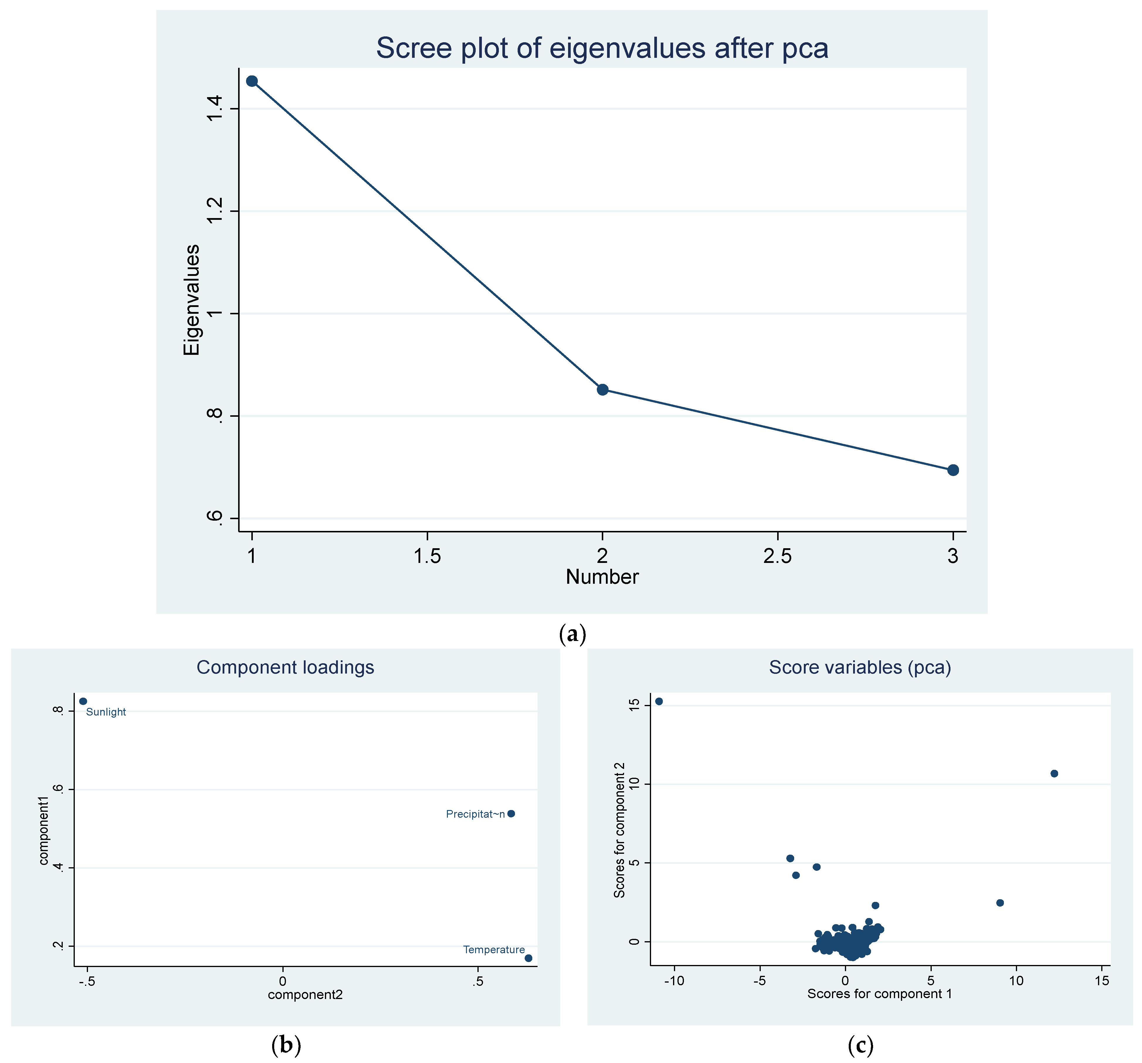
Sunlight hours	−0.5177	0.8152	0.2598

displays the essential components of Climate Index1, generated from three significant climate factors: temperature, precipitation, and sunlight hours. The findings indicate that the initial component possesses eigenvalues of 1.47419. Conversely, the value of the second component is 0.840774, exhibiting a consistent decline until the third component, which manifests a negligible deviation of 0.685034%. The statistics indicate that the initial component demonstrates the greatest degree of variability. However, the subsequent section of Table 2 presents the eigenloadings, which are negative and statistically insignificant. This research aims to generate the Climatic Index1 by utilizing Comp-1.

To obtain comprehensive results, the research employed the four primary components of the Climate Index2: temperature, precipitation, sunlight hours, and CO₂, as illustrated in

Table 3. PCA of Climate Index2.

Component	Eigenvalue	Difference	Proportion	Cumulative
Comp1	1.48648	0.513022	0.3716	0.3716
Comp2	0.973458	0.126635	0.2434	0.615
Comp3	0.846823	0.153583	0.2117	0.8267
Comp4	0.693239	.	0.1733	1
Variable (s)	Comp1	Comp2	Comp3	Comp4
Temperature	0.6068	0.1696	0.2075	0.7483
Precipitation	0.5751	0.0045	0.5378	−0.6165
Sunlight hours	−0.4884	−0.2693	0.7956	0.2365
CO2	−0.2501	0.948	0.1864	−0.0638

. The essential components of Climate Index2 are presented in Table 3. The findings indicate that the initial component possesses an eigenvalue of 1.48648. Conversely, the value of the second component is 0.973458, and it decreases gradually until it reaches the fourth component, which fluctuates by a negligible amount of 0.693239%. The statistics indicate that the initial component demonstrates the greatest degree of variability. Nevertheless, the minimal loadings are denoted by the eigenloads presented in the subsequent section of Table 3. The results of the scree plot, component loading, and score variables (PCA) tests for Climate Index1, shown in Figure 5a–c. While the scree plot, component loading, and score variables for Climate Index2, given in Figure 6a–c. PCA shows that Comp-1 was the right choice for Climate Index1 and Climate Index2. The overarching objective of this study is thus to develop the Climate Index2 utilizing Comp-1 in preparation for the present examination.

4.3. Findings of Econometrics Primary Evaluation

Correlation is utilized to assess the initial state of the parameters. The correlation assessment is outlined in

Table 4. Correlation matrix analysis.

Variable (s)	FE	Temp	Precp	SH	CO2	GDP	GDP2	Tech1	Tech2	Urb	CF Index1	CF Index2
FE	1
Temp	0.392	1
Precp	0.2525	0.2505	1
SH	−0.1867	−0.1902	−0.137	1
CO2	−0.0563	−0.0778	−0.1242	0.0318	1
GDP	0.0494	−0.0142	−0.031	0.0717	0.2285	1
GDP2	−0.041	−0.0107	−0.0397	0.0607	0.2316	0.9488	1
Tech1	0.1941	0.1175	0.0722	−0.0577	0.0716	0.2828	0.2199	1
Tech2	0.3571	0.1777	0.1002	−0.0787	0.1221	0.3577	0.3687	0.0593	1
Urb	−0.3088	−0.0168	−0.0004	0.0614	−0.0217	−0.3702	−0.3173	0.0337	−0.5345	1
CF Index1	0.2525	0.2505	1	−0.137	−0.1242	−0.031	−0.0397	0.0722	0.1002	−0.0004	1
CF Index2	−0.4057	0.7076	0.697	−0.5875	−0.3161	−0.0989	−0.0974	0.1026	0.1443	−0.0299	0.697	1

. The results indicate that temperature and precipitation have a positive impact on enhancing forest productivity. There is a negative association between sunlight hours and CO₂ levels in forests. The initial level of economic development, as measured by GDP, exhibits a positive association, whereas further development demonstrates a negative correlation. Greater technological progress may align with a higher occurrence rate and enhanced efficiency in forest management. Furthermore, there exists a robust positive/negative correlation between CF Index1 and CF Index2, suggesting a high degree of consistency between two distinct measures of a certain variable. Overall, the correlation matrix provides valuable insights into the interdependencies among the analyzed variables, identifying prospective topics for future inquiry or analysis.

We utilized CD for the determination of cross-sectional properties. This stage enables the identification of feasible methodologies for analyzing stationarity and calculating long-term parameters. The estimations are displayed in

Table 5. Findings of cross-dependence (CD) test.

Variable (s)	CD (2004)	p-Value
FE	11.567	0.000
Temp	13.132	0.000
Precp	4.803	0.000
SH	4.822	0.000
CO2	75.545	0.000
CF Index1	4.804	0.000
CF Index2	6.373	0.000
GDP	87.96	0.000
GDP2	85.542	0.000
Tech1	71.837	0.000
Tech2	67.278	0.000
Urb	78.904	0.000

. The findings of the CD tests refute the absence of the CD in the dataset and establish a link within the data. The findings indicate that the policies implemented by the provinces’ economy have a ripple effect, highlighting the importance for countries to be cautious in their policy development. In addition, we conducted separate tests (

Table 6. Findings of slope heterogeneity (SH) analysis.

Slope Homogeneity
Model Tested	Climate to Forest Efficiency Model1		Climate to Forest Efficiency Model2		Forest Efficiency to Climate Model3
Test	∆	Adj.∆	∆	Adj.∆	∆	Adj.∆
Statistics	12.889	14.506	11.686	13.614	10.350	12.058
p-value	0.000	0.000	0.000	0.000	0.000	0.000

) on the three models to assess the homogeneity of their slopes. The results show that the models’ slopes are not uniform, therefore disproving the hypothesis of homogeneous slopes. The analysis of the data on cross-sectional dependence and slope heterogeneity (SH) has given enough information to select the subsequent econometric series.

Thus, we utilized the IPS and CIPS tests to examine panel unit roots. Based on the statistics presented in

Table 7. Findings of unit root analysis.

Variable (s)	I.P.S. Unit Root Test				CIPS Unit Root Test
	Statistics	p-Value	Statistics	p-Value	Level	First Diff	Order I (1)
FE	2.1222	1.0000	−3.0345	0.0000	−2.388	−4.556	Yes
Temp	0.3160	0.6240	−9.9929	0.0000	−2.260	−4.649	Yes
Precp	−0.1212	0.4518	−3.1089	0.0009	−1.987	−4.629	Yes
SH	0.5631	0.7133	−7.8220	0.0000	−2.029	−4.489	Yes
CO2	−0.6340	0.2630	−5.1836	0.0000	−1.463	−3.664	Yes
CF Index1	−0.2742	0.3920	−5.2452	0.0000	−2.051	−5.712	Yes
CF Index2	−1.0970	0.1363	−3.4894	0.0002	−1.903	−3.535	Yes
GDP	0.7634	1.0000	−3.2391	0.0000	−1.016	−3.129	Yes
GDP2	5.2731	1.0000	−13.2442	0.0000	−1.406	−3.560	Yes
Tech1	15.3119	1.0000	−2.3455	0.0095	−2.140	−3.585	Yes
Tech2	−1.0519	0.1464	−5.9803	0.0000	−1.185	−4.254	Yes
Urb	0.3158	0.6239	−2.3490	0.0094	−2.089	−3.613	Yes

, the variables show unit roots at the level but display stationary features when exposed to the first difference testing. Therefore, it may be concluded that the chosen series exhibits characteristics of first-order stationarity. Based on data that showed cross-sectional correlation, diverse slopes, and unit roots in the series, we used the method described by Westerlund to perform co-integration tests. There is a long-standing relationship between these factors (

Table 8. Findings of co-integration analysis.

Westerlund ECM Panel Cointegration Tests (2008)
Model Tested	Climate to Forest Efficiency Model1				Climate to Forest Efficiency Model2				Forest Efficiency to Climate Model3
Statistics	Gt	Ga	Pt	Pa	Gt	Ga	Pt	Pa	Gt	Ga	Pt	Pa
Value	−2.908	−4.005	−2.908	−3.531	−2.806	−3.351	−12.620	−3.153	−2.261	−6.044	−10.538	−5.123
Z-Value	−3.817	5.506	−3.817	3.100	−3.272	5.973	−1.894	3.360	−2.949	1.549	−2.537	−0.740
p-value	0.000	1.000	0.000	0.999	0.001	1.000	0.029	1.000	0.002	0.939	0.006	0.230

).

4.4. Findings of Long-Run Analysis

CupFM and CupBC were chosen for the long-run study’s findings because of their superior characteristics in comparison to other traditional estimators. The obtained results from these estimators are presented in

Table 9. Impact of Climate Index1 on FE.

Variable (s)	Dependent Variable (Forest Efficiency)
	CupFM				CupBC
Temp	0.292 ***			0.172 ***	0.103 ***
	(6.63)			(4.75)	(4.17)
Precp		0.23 5 ***		0.248 ***	0.237 ***
		(10.49)		(9.32)	(9.87)
SH			−0.0697 *	−0.279 ***	−0.0729 ***
			(−1.69)	(−5.12)	(−3.43)
GDP	5.312 ***	5.234 ***	7.426 ***	3.339 ***	2.517 *
	(4.31)	(4.62)	(5.87)	(3.34)	(1.79)
GDP2	−0.234 ***	−0.233 ***	−0.329 ***	−0.145 ***	−0.115 *
	(−4.07)	(−4.38)	(−5.54)	(−3.10)	(−1.81)
Tech1	0.0423 ***	0.0421 ***	0.0931 ***	0.0378 ***	0.0748 ***
	(4.02)	(4.22)	(10.55)	(3.63)	(7.48)
Tech2	0.0334 *	0.0451 ***	0.0388 *	0.0417 ***	0.0728 ***
	(1.65)	(2.63)	(1.83)	(2.85)	(3.46)
Urb	−0.0610	−0.132	−0.191 ***	−0.136 *	−0.00261 ***
	(−0.98)	(−1.51)	(−2.98)	(−1.64)	(−3.23)
CF Index1				0.765 ***	0.228 ***
				(10.06)	(9.87)
Number of groups	30	30	30	30	30

Note: t-values in parentheses *** p < 0.01, * p < 0.1.

. Initially, when considering FE as the dependent variable, we assessed each climate factor (temperature, precipitation, and sunlight hours (column 1 to column 4)) individually.

The results showed that temperature tends to escalate the FE of Chinese provinces by 0.292%, which is in line with Collalti et al. (2020) [49].

In column 2, findings show that a 1% increase in precipitation would raise the FE by 0.235%. These results are in line with (Collalti et al. 2020; Sheil., 2018; Xu et al. 2024) [49,50,51], who stated that precipitation is important for forests. Increased precipitation can boost FE in Chinese regions. For instance, sufficient precipitation allows trees to maintain photosynthesis and transpiration by providing moisture. This boosts biomass output and forest health. Furthermore, precipitation refills soil moisture, which tree roots need to absorb and cycle nutrients. Precipitation increases forest biodiversity and ecological resilience. However, sunlight hours do not positively increase the FE, indicating that a 1% increase in sunlight would lower the efficiency of the forest by −0.0697%.

Subsequently, we composed the Climate Index1 (CF Index1) using three climate factors to assess the communal effects of climate. The results showed that the overall impact of Climate Index1 is positive. It implies that a 1% increase in precipitation, sunlight hours, and temperature would increase the FE by 0.765%.

Rapid economic growth often occurs in tandem with the depletion of forest resources. Thus, the non-linear impact of economic growth in the lens of EKC is observed. The results showed that continuous economic growth is unfavorable for FE, as the initial impact is positive, but the later effect is negative. As an example, column 1 findings showed that a 1% increase in economic growth may lead to a boost in FE by 5.312% at the initial level. However, the economic development the FE would be decreased by −0.234%. In other words, the study finds an inverted U-shaped Kuznets curve. The results can be verified with Hao et al. (2019) [36]. The impact of technology (Tech1) in terms of research and development on FE is positive, indicating a 1% increase in research and development activities would increase the FE by 0.04% in column 1. Similarly, the forest-based investment (Tech2) is significantly positive to escalate the FE of the Chinese province by 0.0334%. These findings can be robust with Venanzi et al. (2023) [52], who argued that technology can be effective in improving the efficiency of forests by managing and monitoring forest activity. Further, El-Lakany et al. (2001) [53] backed our study findings as they highlighted that technological developments have had a constructive impact on forest areas and conditions. In contrast, the urbanization expansion significantly harms the efficiency of forests. A 1% increase in urbanization would reduce the FE by −0.06% to 0.1% (columns 1–4). These results are in line with (Zhang et al., 2020) [54].

Climate Index1 did not consider carbon emission impact, which is a significant factor in climate. Thus, we estimate the Climate Index2 (CF Index2) with CO₂ and the findings described in

Table 10. Impact of Climate Index2 on FE.

Variable (s)	Dependent (Forest Efficiency)
	CupFM		CupBC
GDP	−0.125 ***	0.0431 ***	0.0431 ***
	(−3.52)	(3.62)	(4.18)
GDP2		−0.0546 ***	−0.107 ***
		(−6.18)	(−3.71)
Tech1	0.125 ***	0.131 ***	0.0823 ***
	(17.80)	(23.35)	(10.03)
Tech2	0.0113	0.00924 **	0.103 ***
	(1.52)	(1.99)	(4.17)
Urb	0.0247	0.00107	0.143 **
	(0.53)	(0.02)	(2.80)
CO2	−0.0987 ***	−0.110 ***	−0.0701 ***
	(−8.43)	(−8.87)	(−6.87)
CF Index2		−0.0748 ***	−0.0776 **
		(−7.48)	(−2.21)
Number of groups	30	30	30

Note: t-values in parentheses *** p < 0.01, ** p < 0.05.

. First, the individual impact of carbon emission (CO₂) on FE is negative, indicating that a 1% increase in carbon emission would decrease the FE by −0.0987% to −0.110%. Further, the index also showed a negative influence (−0.0748%) towards FE after the insertion of CO₂. Table 10 findings are again indorsed an inverted U-shaped Kuznets curve, as the initial impact of economic growth is positive and later is negative. Technology is found to be positive for the increase of FE, consistent with previous findings.

Simultaneously, forests are also important to improve the climate condition. Considering this, the study evaluates the FE impact for improving climate conditions. The climate index (temperature, precipitation, sunlight hours, and CO₂) is the dependent variable. The results described in

Table 11. Impact of FE on climate change.

Variable (s)	Dependent Variable (Climate Index)
	CupFM	CupBC
FE	−1.512 ***	−1.520 ***
	(−9.27)	(−9.10)
GDP	0.0728 ***	0.237 ***
	(3.46)	(9.87)
GDP2	−0.00274 ***	−0.0701 ***
	(−3.56)	(−6.87)
Tech1	−0.0972 **	−0.0925 **
	(−2.41)	(−2.34)
Tech2	−0.104 **	−0.104 **
	(−2.69)	(−2.57)
Urb	0.687 **	0.670 ***
	(2.83)	(2.93)
Number of groups	30	30

Note: t-values in parentheses *** p < 0.01, ** p < 0.05.

showed that forests positively increase climate quality by controlling carbon emissions and other factors. It implies that a 1% increase in FE would lead to improve the climate quality by −1.512%. UNDP [55] asserts that healthy forests have a significant impact on climate change mitigation through their function as carbon sinks, effectively absorbing billions of metric tons of CO₂ on an annual basis. The study found the inverted U-shaped EKC of climate at an earlier stage as economic growth increases the climate factors in terms of temperature, carbon, precipitation, and sunlight, reducing the air atmosphere’s climate quality. At the same time, the later phase of development positively impacts climate by reducing the negative effects of climate factors. Similar to previous findings, technology impact is positive to improve the climate quality. A 1% increase in Tech1 and Tech2 would reduce the negative impact of climate factors by −0.0972% and −0.104%, respectively. In contrast, urbanization reduces the climate quality by 0.687%.

Long-Run Findings Discussion

The long-run findings from Table 9, Table 10 and Table 11 highlight the significance of climate factors, economic growth, technology, urbanization, and carbon emissions in shaping China’s FE and climate quality. However, the influencing dynamics of these factors are different.

For instance, through the lens of findings, we assessed that temperature and precipitation are positive drivers rather than sunlight in enhancing China’s FE. For instance, China has diverse climatic regions that can exhibit varied responses to temperature, precipitation, and sunlight hours. The findings indicate that temperature escalation positively impacts FE, maybe in regions where extended growing seasons facilitate increased biomass production. Warmer temperatures promote organic matter decomposition, releasing nutrients into the soil and promoting nutrient cycling, which is essential for forest productivity [56]. However, temperature escalation may initially increase FE, but it may also worsen water stress and pest outbreaks, requiring careful management to maintain forest health and productivity. Precipitation increases FE by providing moisture for photosynthesis, transpiration, and nutrient cycling. Sunlight hours, however, do not significantly affect FE. Although sunlight is essential for forest ecosystems, its impacts on efficiency vary depending on forest layout, plant species composition, and weather.

China’s rapid economic growth has historically been associated with environmental degradation, including deforestation and habitat loss. The inverted U-shaped Kuznets curve illustrates the initial positive impact of economic growth to some extent on FE, followed by a decline as urbanization and industrialization intensify. According to our study, continuing economic growth and urbanization can be the reasons for decreasing FE in China. It implies that the economic development of China puts pressure on forest resources. Economic development is a primary goal of China as well as local areas and brings economic development and population aggregation through the consumption of multiple resources. Our study can be backed by Hao et al. (2019) [36], who found that with continuous economic growth, the timber output and area of afforestation would at first increase and then decrease after reaching the corresponding turning points. Higher GDP levels are commonly linked to heightened industrialization, greater energy usage, and increased emissions of greenhouse gases, hence contributing to the global temperature increase caused by the intensified greenhouse effect (Leal and Marques, 2022) [57].

Moreover, economic activities have the potential to impact precipitation patterns through land changes. Further, economic development can indirectly impact sunlight hours through weather changes. In addition, there is generally a positive correlation between GDP growth and CO₂ emissions unless there are improvements in energy efficiency and the implementation of renewable energy sources to reduce emissions. The increasing population in hillside and mountainous regions has been a major driver of deforestation throughout China’s history. However, technological innovations in forest management offer economic opportunities to enhance FE and mitigate environmental impacts.

This study provides condensed evidence about carbon’s role in FE. The efficacy of forests has a substantial impact on climate dynamics, as it regulates temperature, patterns of precipitation, duration of sunlight, and levels of CO₂. Forests function as natural climate regulators by utilizing photosynthesis to absorb CO₂, aiding in the reduction of greenhouse gas emissions and maintaining stable levels of atmospheric carbon. In addition, trees have an impact on the distribution of rainfall in nearby areas by recycling water vapor through transpiration and aiding in the creation of clouds. Modifications in FE such as the removal of trees or the establishment of new forests, have the potential to disturb these processes, resulting in changes in temperature patterns, adjustments in the distribution of rainfall, and fluctuations in the availability of sunshine. Hence, it is crucial to uphold FE to preserve climate stability and enhance the ability of ecosystems to adapt to continuous environmental changes.

In summary, the general basic loop chain among FE, economic growth, urbanization, climate, and technology is as follows: the interplay among FE, economic growth, urban dynamics, climate, and technology forms an interconnected loop chain with significant implications for socioeconomic and environmental systems. For instance, forest resources, crucial for human sustenance, support population growth by providing essential materials for livelihoods and serving as a foundation for local economies through activities like harvesting and processing. However, rapid population growth can strain resources and lead to environmental degradation. This demographic expansion, in turn, acts as a driving force for economic development, creating demand for labor and stimulating industrial growth, which further attracts population influx. Yet, economic activities associated with this growth such as industrialization and urbanization exert pressure on forest ecosystems and contribute to climate change. Climate variability and extremes, influenced by these activities, impact forests directly, affecting their health, productivity, and distribution.

Consequently, climate-induced disruptions can alter economic activities and population dynamics, necessitating adaptive strategies. However, technological innovations in forest management present opportunities to enhance efficiency and resilience, mitigate environmental impacts, and promote sustainable economic growth. However, their adoption must be carefully implemented, considering economic feasibility and local socio-economic contexts to ensure equitable distribution of benefits and the minimization of adverse environmental consequences. Thus, this loop chain highlights the intricate relationships between human societies, natural ecosystems, and technological advancements in shaping sustainable development pathways for China.

The study findings and discussion can help policymakers understand Chinese provinces’ complicated climate conditions, technology, economic development, and FE connections. The positive impact of temperature and precipitation emphasizes the need to reduce climate change’s negative effects through reforestation and sustainable forest management to preserve and restore forest ecosystems. The study of climate index influence suggests that forests can improve the surrounding environment and help to achieve a lower carbon emission economy. So, forests must be preserved and expanded to reduce the negative effects of urbanization and improve climate quality. For that, policymakers can encourage investment in the forest sector to advance the forest sector and monitor the related activities. Further, there is a dire need to balance economic development and environmental conservation. Forest protection could be part of sustainable development and green growth policies that prioritize ecological integrity and economic progress.

5. Conclusions

The main objective of this study was to evaluate the impact of climate and technology on FE across China provinces during the period spanning from 2002 to 2020. By employing regression techniques such as CupFM and CupBC, our study has generated a number of noteworthy findings. It is worth noting that our findings indicate an encouraging correlation between temperature and precipitation with the enhancement of FE. However, it is also important to highlight that sunlight hours and carbon emissions do not exhibit a substantial contribution towards improving FE.

Additionally, our analysis has shown that Climate Index1 has a positive effect, whereas Climate Index2 has a negative effect, suggesting that forests are essential in improving climate conditions. The results highlight the significance of conserving and improving forest ecosystems as a means of alleviating the impacts of climate change.

Moreover, our research highlights the significance of technical progress in enhancing the efficiency of forests and exerting a positive influence on climatic patterns. Nevertheless, it is imperative to acknowledge the intricate relationship between economic development and the expansion of forests. Based on our analysis, it is evident that technological developments have the potential to enhance FE. However, the influence of economic development, as demonstrated through the lens of EKC, demonstrates a non-linear relationship characterized by an inverted U-shaped pattern. Consequently, although the first economic activities may have a positive impact on the growth of forests, ongoing economic expansion may have adverse consequences on forest ecosystems.

In a similar vein, our analysis of the environmental Kuznets curve with respect to climate conditions demonstrates an inverted U-shaped EKC pattern, underscoring the complex nature of the relationship between economic development and environmental sustainability.

Moreover, urbanization is identified as a prominent determinant that contributes to decreased FE as a result of population expansion and the accompanying human endeavors. It highlights the importance of implementing sustainable urban planning and forest conservation initiatives to address the negative consequences of urban growth on forest ecosystems.

In summary, our research offers unique insights that have substantial consequences for the management of forests, the mitigation of climate change, and the formulation of sustainable development strategies. Policymakers can strengthen their abilities to promote forest conservation and enhance environmental sustainability by comprehending the complex dynamics of climate, technology, economic development, and urbanization.

References

- Liang, B.; Wang, J.; Zhang, Z.; Zhang, J.; Zhang, J.; Cressey, E.L.; Wang, Z. Planted forest is catching up with natural forest in China in terms of carbon density and carbon storage. Fundam. Res. 2022, 2, 688–696. [Google Scholar] [CrossRef]
- Farooq, T.H.; Shakoor, A.; Wu, X.; Li, Y.; Rashid, M.H.U.; Zhang, X.; Gilani, M.M.; Kumar, U.; Chen, X.; Yan, W. Perspectives of plantation forests in the sustainable forest development of China. Iforest-Biogeosci. For. 2021, 14, 166–174. [Google Scholar] [CrossRef]
- Liu, J.; Reddy, R.C.; Liu, X.; Zhao, X.; Li, X.; Chen, Y. Review on Sustainable Forest Management and Financing in China. In Review on Sustainable Forest Management and Financing in China (English); World Bank Group: Washington, DC, USA, 2019; Available online: http://documents.worldbank.org/curated/en/794721572413296261/Review-on-Sustainable-Forest-Management-and-Financing-in-China (accessed on 15 March 2024).
- McDowell, N.G.; Allen, C.D.; Anderson-Teixeira, K.; Aukema, B.H.; Bond-Lamberty, B.; Chini, L.; Clark, J.S.; Dietze, M.; Grossiord, C.; Hanbury-Brown, A.; et al. Pervasive shifts in forest dynamics in a changing world. Science 2020, 368, eaaz9463. [Google Scholar] [CrossRef]
- Nunes, L.J.; Meireles, C.I.; Gomes, C.J.P.; Ribeiro, N.M.A. The impact of climate change on forest development: A sustainable approach to management models applied to Mediterranean-type climate regions. Plants 2021, 11, 69. [Google Scholar] [CrossRef] [PubMed]
- Dusenge, M.E.; Duarte, A.G.; Way, D.A. Plant carbon metabolism and climate change: Elevated CO2 and temperature impacts on photosynthesis, photorespiration and respiration. New Phytol. 2019, 221, 32–49. [Google Scholar] [CrossRef]
- Hui, D.; Deng, Q.; Tian, H.; Luo, Y. Climate change and carbon sequestration in forest ecosystems. Handb. Clim. Change Mitig. Adapt. 2017, 555, 594. [Google Scholar]
- Henne, P.D.; Hawbaker, T.J.; Scheller, R.M.; Zhao, F.; He, H.S.; Xu, W.; Zhu, Z. Increased burning in a warming climate reduces carbon uptake in the Greater Yellowstone Ecosystem despite productivity gains. J. Ecol. 2021, 109, 1148–1169. [Google Scholar] [CrossRef]
- Jactel, H.; Petit, J.; Desprez-Loustau, M.L.; Delzon, S.; Piou, D.; Battisti, A.; Koricheva, J. Drought effects on damage by forest insects and pathogens: A meta-analysis. Glob. Chang. Biol. 2012, 18, 267–276. [Google Scholar] [CrossRef]
- Shi, M.; Qi, J.; Yin, R. Has China’s natural forest protection program protected forests?—Heilongjiang’s experience. Forests 2016, 7, 218. [Google Scholar] [CrossRef]
- Bernal, B.; Murray, L.T.; Pearson, T.R. Global carbon dioxide removal rates from forest landscape restoration activities. Carbon Balance Manag. 2018, 13, 1–13. [Google Scholar] [CrossRef]
- Nowak, D.J.; Dwyer, J.F. Understanding the benefits and costs of urban forest ecosystems. In Urban and Community Forestry in the Northeast; Springer Netherlands: Dordrecht, The Netherlands, 2007; pp. 25–46. [Google Scholar]
- Wang, S.; Zhang, Y.; Ju, W.; Chen, J.M.; Ciais, P.; Cescatti, A.; Sardans, J.; Janssens, I.A.; Wu, M.; Berry, J.A.; et al. Recent global decline of CO2 fertilization effects on vegetation photosynthesis. Science 2020, 370, 1295–1300. [Google Scholar] [CrossRef]
- Robredo, A.; Pérez-López, U.; de la Maza, H.S.; González-Moro, B.; Lacuesta, M.; Mena-Petite, A.; Muñoz-Rueda, A. Elevated CO2 alleviates the impact of drought on barley improving water status by lowering stomatal conductance and delaying its effects on photosynthesis. Environ. Exp. Bot. 2007, 59, 252–263. [Google Scholar] [CrossRef]
- Reyer, C.P.; Bathgate, S.; Blennow, K.; Borges, J.G.; Bugmann, H.; Delzon, S.; Faias, S.P.; Garcia-Gonzalo, J.; Gardiner, B.; Gonzalez-Olabarria, J.R.; et al. Are forest disturbances amplifying or canceling out climate change-induced productivity changes in European forests? Environ. Res. Lett. ERL [Web Site] 2017, 12, 034027. [Google Scholar] [CrossRef]
- Addas, A. Impact of forestry on environment and human health: An evidence-based investigation. Front. Public Health 2023, 11, 1260519. [Google Scholar] [CrossRef]
- Torun, P.; Altunel, A.O. Effects of environmental factors and forest management on landscape-scale forest storm damage in Turkey. Ann. For. Sci. 2020, 77, 39. [Google Scholar] [CrossRef]
- Boisvenue, C.; Running, S.W. Impacts of climate change on natural forest productivity–evidence since the middle of the 20th century. Glob. Chang. Biol. 2006, 12, 862–882. [Google Scholar] [CrossRef]
- García-Valdés, R.; Estrada, A.; Early, R.; Lehsten, V.; Morin, X. Climate change impacts on long-term forest productivity might be driven by species turnover rather than by changes in tree growth. Glob. Ecol. Biogeogr. 2020, 29, 1360–1372. [Google Scholar] [CrossRef]
- Pecchi, M.; Marchi, M.; Giannetti, F.; Bernetti, I.; Bindi, M.; Moriondo, M.; Maselli, F.; Fibbi, L.; Corona, P.; Travaglini, D.; et al. Reviewing climatic traits for the main forest tree species in Italy. Iforest-Biogeosci. For. 2019, 12, 173. [Google Scholar] [CrossRef]
- Soucy, A.; De Urioste-Stone, S.; Rahimzadeh-Bajgiran, P.; Weiskittel, A.; McGreavy, B. Forestry professionals’ perceptions of climate change impacts on the forest industry in Maine, USA. J. Sustain. For. 2021, 40, 695–720. [Google Scholar] [CrossRef]
- Wei, J.; Shen, M. Analysis of the efficiency of forest carbon sinks and its influencing factors—Evidence from China. Sustainability 2022, 14, 11155. [Google Scholar] [CrossRef]
- García, C.; Espelta, J.M.; Hampe, A. Managing forest regeneration and expansion at a time of unprecedented global change. J. Appl. Ecol. 2020, 57, 2310–2315. [Google Scholar] [CrossRef]
- Gavilanes Montoya, A.V.; Castillo Vizuete, D.D.; Marcu, M.V. Exploring the Role of ICTs and Communication Flows in the Forest Sector. Sustainability 2023, 15, 10973. [Google Scholar] [CrossRef]
- Li, L.; Hao, T.; Chi, T. Evaluation on China’s forestry resources efficiency based on big data. J. Clean. Prod. 2017, 142, 513–523. [Google Scholar] [CrossRef]
- Cheng, S.; Xu, Z.; Su, Y.; Zhen, L. Spatial and temporal flows of China’s forest resources: Development of a framework for evaluating resource efficiency. Ecol. Econ. 2010, 69, 1405–1415. [Google Scholar] [CrossRef]
- Zhang, Z.; Zhang, C. Revisiting the importance of forest rents, oil rents, green growth in economic performance of China: Employing time series methods. Resour. Policy 2023, 80, 103140. [Google Scholar] [CrossRef]
- Djafar, E.M.; Widayanti, T.F.; Saidi, M.D.; Muin, A.M. Forest management to Achieve Sustainable Forestry Policy in Indonesia. In IOP Conference Series: Earth and Environmental Science; IOP Publishing: Bristol, UK, 2023; Volume 1181, p. 012021. [Google Scholar]
- Yilanci, V.; Ulucak, R.; Zhang, Y.; Andreoni, V. The role of affluence, urbanization, and human capital for sustainable forest management in China: Robust findings from a new method of Fourier co-integration. Sustain. Dev. 2023, 31, 812–824. [Google Scholar] [CrossRef]
- Ali, S.; Wang, D.; Hussain, T.; Lu, X.; Nurunnabi, M. Forest resource management: An empirical study in Northern Pakistan. Sustainability 2021, 13, 8752. [Google Scholar] [CrossRef]
- He, Y.; Ren, Y. Can carbon sink insurance and financial subsidies improve the carbon sequestration capacity of forestry? J. Clean. Prod. 2023, 397, 136618. [Google Scholar] [CrossRef]
- Pesaran, M.H.; Yamagata, T. Testing slope homogeneity in large panels. J. Econom. 2008, 142, 50–93. [Google Scholar] [CrossRef]
- Pearson, K. On lines and planes of closest fit to systems of points in space. Lond. Edinb. Dublin Philos. Mag. J. Sci. 1901, 2, 559–572. [Google Scholar] [CrossRef]
- Hotelling, H. Analysis of a complex of statistical variables into principal components. J. Educ. Psychol. 1933, 24, 417. [Google Scholar] [CrossRef]
- García-Sánchez, E.; García-Morales, V.J.; Martín-Rojas, R. Analysis of the influence of the environment, stakeholder integration capability, absorptive capacity, and technological skills on organizational performance through corporate entrepreneurship. Int. Entrep. Manag. J. 2018, 14, 345–377. [Google Scholar] [CrossRef]
- Hao, Y.; Xu, Y.; Zhang, J.; Hu, X.; Huang, J.; Chang, C.P.; Guo, Y. Relationship between forest resources and economic growth: Empirical evidence from China. J. Clean. Prod. 2019, 214, 848–859. [Google Scholar] [CrossRef]
- Liu, W.; Zhan, J.; Zhao, F.; Yan, H.; Zhang, F.; Wei, X. Impacts of urbanization-induced land-use changes on ecosystem services: A case study of the Pearl River Delta Metropolitan Region, China. Ecol. Indic. 2019, 98, 228–238. [Google Scholar] [CrossRef]
- Tone, K.A. Slacks-Based Measure of Super-Efficiency in Data Envelopment Analysis. Eur. J. Oper. Res. 2002, 204, 694–697. [Google Scholar] [CrossRef]
- Pesaran, M.H. Estimation and inference in large heterogeneous panels with a multifactor error structure. Econometrica 2006, 74, 967–1012. [Google Scholar] [CrossRef]
- Pesaran, M.H. General diagnostic tests for cross section dependence in panels. Empir. Econ. 2004, 60, 13–50. [Google Scholar] [CrossRef]
- Koçak, E.; Ulucak, R.; Ulucak, Z.Ş. The impact of tourism developments on CO2 emissions: An advanced panel data estimation. Tour. Manag. Perspect. 2020, 33, 100611. [Google Scholar] [CrossRef]
- Im, K.S.; Pesaran, M.H.; Shin, Y. Testing for unit roots in heterogeneous panels. J. Econom. 2003, 115, 53–74. [Google Scholar] [CrossRef]
- Pesaran, M.H. A simple panel unit root test in the presence of cross-section dependence. J. Appl. Econom. 2007, 22, 265–312. [Google Scholar] [CrossRef]
- Hatemi-j, A. Tests for co-integration with two unknown regime shifts with an application to financial market integration. Empir. Econ. 2008, 35, 497–505. [Google Scholar] [CrossRef]
- Phillips, P.C.; Sul, D. Dynamic panel estimation and homogeneity testing under cross section dependence. Econom. J. 2003, 6, 217–259. [Google Scholar] [CrossRef]
- Westerlund, J. Panel co-integration tests of the Fisher effect. J. Appl. Econom. 2008, 23, 193–233. [Google Scholar] [CrossRef]
- Bai, J.; Kao, C. On the estimation and inference of a panel co-integration model with cross-sectional dependence. Contrib. Econ. Anal. 2006, 274, 3–30. [Google Scholar]
- Bai, J.; Kao, C.; Ng, S. Panel co-integration with global stochastic trends. J. Econom. 2009, 149, 82–99. [Google Scholar] [CrossRef]
- Collalti, A.; Ibrom, A.; Stockmarr, A.; Cescatti, A.; Alkama, R.; Fernández-Martínez, M.; Matteucci, G.; Sitch, S.; Friedlingstein, P.; Ciais, P.; et al. Forest production efficiency increases with growth temperature. Nat. Commun. 2020, 11, 5322. [Google Scholar] [CrossRef]
- Sheil, D. Forests, atmospheric water and an uncertain future: The new biology of the global water cycle. For. Ecosyst. 2018, 5, 1–22. [Google Scholar] [CrossRef]
- Xu, S.; Wang, J.; Sayer, E.J.; Lam, S.K.; Lai, D.Y. Precipitation change affects forest soil carbon inputs and pools: A global meta-analysis. Sci. Total Environ. 2024, 908, 168171. [Google Scholar] [CrossRef]
- Venanzi, R.; Latterini, F.; Civitarese, V.; Picchio, R. Recent Applications of Smart Technologies for Monitoring the Sustainability of Forest Operations. Forests 2023, 14, 1503. [Google Scholar] [CrossRef]
- EL-Lakany, M.H.; Ball, J. Technology and the forest landscape: Rapid changes and their real impacts. Int. For. Rev. 2001, 3, 184–187. [Google Scholar]
- Zhang, W.; Ma, J.; Liu, M.; Li, C. Impact of urban expansion on forest carbon sequestration: A study in Northeastern China. Pol. J. Environ. Stud. 2020, 29, 451–461. [Google Scholar] [CrossRef]
- United Nations Development Programme (UNDP). Forests can Help Us Limit Climate Change–Here Is How. 2023. Available online: https://climatepromise.undp.org/news-and-stories/forests-can-help-us-limit-climate-change-here-how#:~:text=Healthy%20forests%20play%20a%20crucial,achieving%20the%20world’s%20climate%20goals (accessed on 10 April 2024).
- Saha, S.; Huang, L.; Khoso, M.A.; Wu, H.; Han, D.; Ma, X.; Poudel, T.R.; Li, B.; Zhu, M.; Lan, Q.; et al. Fine root decomposition in forest ecosystems: An ecological perspective. Front. Plant Sci. 2023, 14, 1277510. [Google Scholar] [CrossRef]
- Leal, P.H.; Marques, A.C. The evolution of the environmental Kuznets curve hypothesis assessment: A literature review under a critical analysis perspective. Heliyon 2022, 8, e11521. [Google Scholar] [CrossRef]
Figure 1.
Forest Efficiency (dependent variable) trend for Year 2020.
Figure 2.
Independent variables trends of all provinces for 2020.
Figure 3.
FE trend from 2002 to 2020 by province. Note: measured by SBM-DEA.
Figure 4.
Average FE of Chinese regions from 2002 to 2020 (Tibet excluded).
Figure 5.
(a). Scree plot of eigenvalues for Climate Index1. (b) Component loading plot for Climate Index1. (c) Score variables (PCA) for Climate Index1.
Figure 6.
(a). Scree plot of eigenvalues for Climate Index2. (b) Component loading plot for Climate Index1. (c) Score variables (PCA) for Climate Index1.