
Detecting Local Drivers of Fire Cycle Heterogeneity in Boreal Forests: A Scale Issue


 ,
,
Abstract
:
1. Introduction
2. Materials and Methods
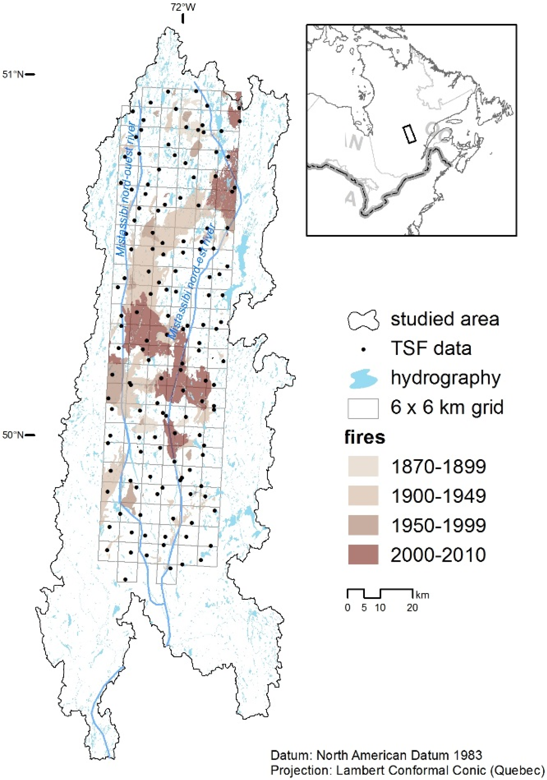
2.1. Study Area
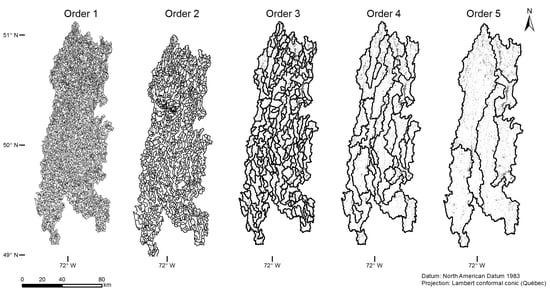
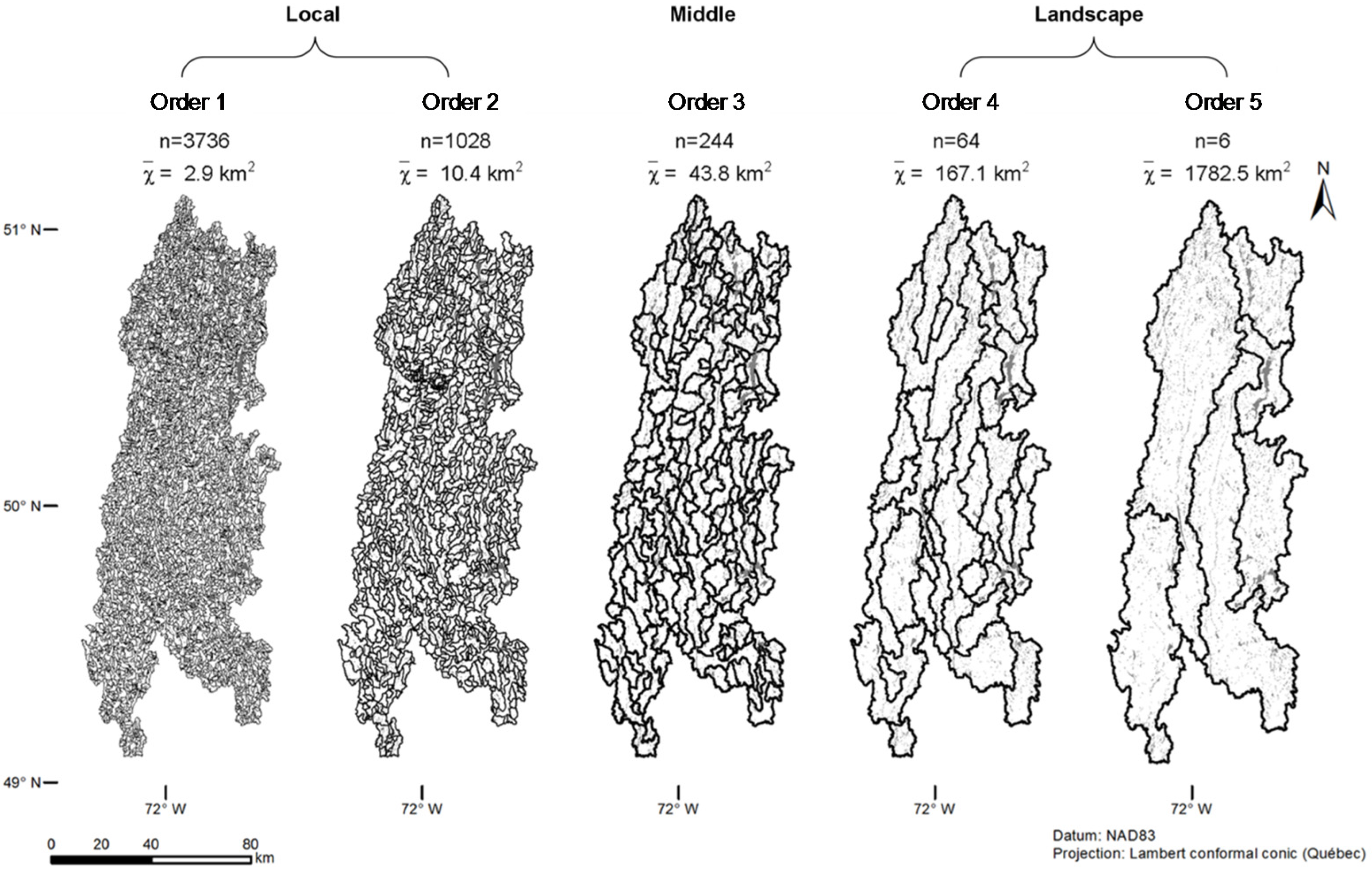
2.2. Environment Delineation and Scaling
2.3. Data Collection
2.4. Survival Analysis
2.5. FC Prediction and Distribution
2.6. Vegetation Composition
3. Results
3.1. Time since Fire Distribution
3.2. FC Modeling
3.3. FC Distribution
3.4. Model Validation
3.5. FC and Succession Pathways
4. Discussion
4.1. FC Physical Drivers and Scales
4.2. A Local FC Model
4.3. Model Validation
4.4. FC and Vegetation
4.5. Implications for Forest Management
5. Conclusions
Acknowledgments
Author Contributions
Conflicts of Interest
Abbreviation
| FC | Fire cycle |
| TSF | Time since last fire |
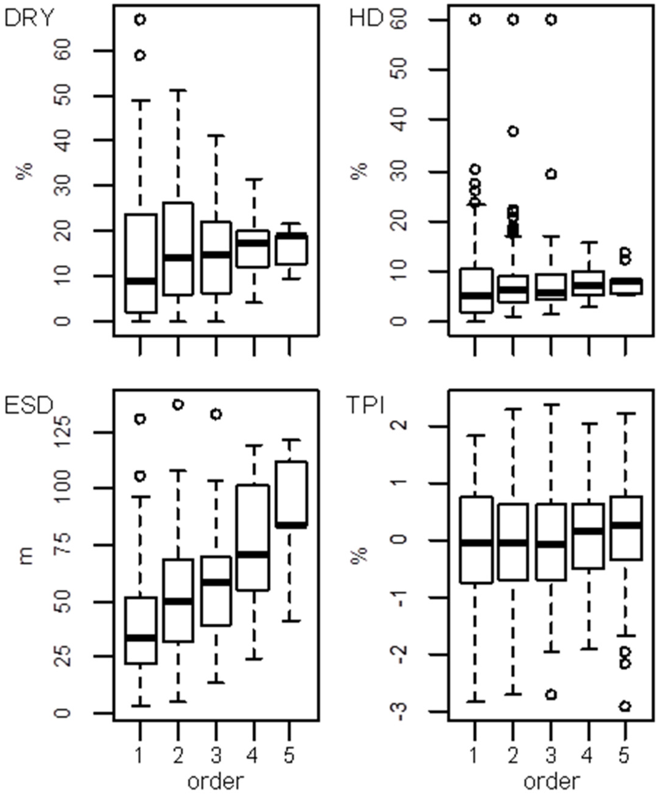
| DRY | Dry surficial deposit density |
| HD | Hydrographic density |
| ESD | Elevation standard deviation |
| TPI | Topographic position index |
Appendix


| Model | Degrees of Freedom | Loglikelihood | AICc | ΔAICc | Weight | |
|---|---|---|---|---|---|---|
| 1 | log(DRY1) + log(DRY3) + HD1 | 3 | −357.8589 | 721.8892 | 0.0000 | 0.0575 |
| 2 | log(DRY3) + HD1 + ESD1 | 3 | −357.8718 | 721.9151 | 0.0259 | 0.0568 |
| 3 | log(DRY1) + log(DRY3)3 + HD1 + ESD1 | 4 | −356.8615 | 722.0108 | 0.1217 | 0.0541 |
| 4 | log(DRY1) + HD1 + ESD3 | 3 | −358.1568 | 722.4850 | 0.5958 | 0.0427 |
| 5 | log(DRY1) + HD1 | 2 | −359.2333 | 722.5517 | 0.6626 | 0.0413 |
| 6 | log(DRY1) + log(DRY3) + HD1 + ESD3 | 4 | −357.1722 | 722.6322 | 0.7430 | 0.0397 |
| 7 | log(DRY1) + log(DRY3) + HD1 + TPI4 | 4 | −357.3373 | 722.9624 | 1.0732 | 0.0336 |
| 8 | log(DRY3) + HD1 + ESD1 + TPI4 | 4 | −357.4987 | 723.2851 | 1.3959 | 0.0286 |
| 9 | log(DRY1) + HD1 + TPI4 | 3 | −358.5942 | 723.3597 | 1.4706 | 0.0276 |
| 10 | log(DRY1) + log(DRY3) + HD1 + ESD1 + TPI4 | 5 | −356.5770 | 723.5888 | 1.6997 | 0.0246 |
| 11 | log(DRY1) + HD1 + ESD3 + TPI4 | 4 | −357.7217 | 723.7312 | 1.8421 | 0.0229 |
| 12 | log(DRY3) + HD1 + HD3 + ESD1 | 4 | −357.7719 | 723.8315 | 1.9423 | 0.0218 |
| 13 | log(DRY1) + HD1 + ESD1 | 3 | −358.8381 | 723.8476 | 1.9584 | 0.0216 |
| 14 | log(DRY3) + HD1 + ESD1 + ESD3 | 4 | −357.7942 | 723.8762 | 1.9870 | 0.0213 |
| 15 | log(DRY1) + log(DRY3) + HD1 + HD3 | 4 | −357.8120 | 723.9117 | 2.0225 | 0.0209 |
References
- Bonan, G.B.; Shugart, H.H. Environmental factors and ecological processes in boreal forests. Annu. Rev. Ecol. Syst. 1989, 20, 1–28. [Google Scholar] [CrossRef]
- Payette, S. Fire as a controlling process in the North American boreal forest. Syst. Anal. Glob. Boreal For. 1992, 144–169. [Google Scholar] [CrossRef]
- Stocks, B.J.; Mason, J.A.; Todd, J.B.; Bosch, E.M.; Wotton, B.M.; Amiro, B.D.; Flannigan, M.D.; Hirsch, K.G.; Logan, K.A.; Martell, D.L.; et al. Large forest fires in Canada, 1959–1997. J. Geophys. Res. 2003, 108, 1–12. [Google Scholar] [CrossRef]
- Johnson, E.A. Fire and Vegetation Dynamics: Studies from the North American Boreal Forest; Cambridge University Press: Cambridge, UK, 1992; p. 129. [Google Scholar]
- Bergeron, Y.; Gauthier, S.; Kafka, V.; Lefort, P.; Lesieur, D. Natural fire frequency for the eastern Canadian boreal forest: Consequences for sustainable forestry. Can. J. For. Res. 2001, 31, 384–391. [Google Scholar] [CrossRef]
- Wu, J.; Loucks, O.L. From balance of nature to hierarchical patch dynamics: A paradigm shift in ecology. Q. Rev. Biol. 1995, 70, 439–466. [Google Scholar] [CrossRef]
- Dix, R.L.; Swan, J.M.A. The roles of disturbance and succession in upland forest at Candle Lake, Saskatchewan. Can. J. Bot. 1971, 49, 657–676. [Google Scholar] [CrossRef]
- Landres, P.B.; Morgan, P.; Swanson, F.J. Overview of the use of natural variability concepts in managing ecological systems. Ecol. Appl. 1999, 9, 1179–1188. [Google Scholar]
- Gauthier, S.; Vaillancourt, M.-A.; Kneeshaw, D.D.; Drapeau, P.; de Grandpré, L.; Claveau, Y.; Paré, D. Forest Ecosystem Management: Origins and Foundations. In Ecosystem Management in the Boreal Forest; Gauthier, S., Vaillancourt, M.-A., Leduc, A., de Grandpré, L., Kneeshaw, D.D., Morin, H., Drapeau, P., Bergeron, Y., Eds.; Les Presses de l’Université du Québec: Quebec, QC, Canada, 2009; pp. 13–38. [Google Scholar]
- Gauthier, S.; Leduc, A.; Bergeron, Y. Forest dynamics modelling under natural fire cycles: A tool to define natural mosaic diversity for forest management. Environ. Monit. Assess. 1996, 39, 417–434. [Google Scholar] [CrossRef] [PubMed]
- Kuuluvainen, T. Natural variability of forests as a reference for restoring and managing biological diversity in boreal Fennoscandia. Silva Fenn. 2002, 36, 97–125. [Google Scholar] [CrossRef]
- Franklin, J.F.; Spies, T.A.; Pelt, R.V.; Carey, A.B.; Thornburgh, D.A.; Berg, D.R.; Lindenmayer, D.B.; Harmon, M.E.; Keeton, W.S.; Shaw, D.C.; et al. Disturbances and structural development of natural forest ecosystems with silvicultural implications, using Douglas-fir forests as an example. For. Ecol. Manag. 2002, 155, 399–423. [Google Scholar] [CrossRef]
- Gauthier, S.; Raulier, F.; Ouzennou, H.; Saucier, J.-P. Strategic analysis of forest vulnerability to risk related to fire: An example from the coniferous boreal forest of Quebec. Can. J. For. Res. 2015, 45, 553–565. [Google Scholar] [CrossRef]
- Vaillancourt, M.-A.; de Grandpré, L.; Gauthier, S.; Leduc, A.; Kneeshaw, D.D.; Claveau, Y.; Bergeron, Y. How can natural disturbances be a guide for forest ecosystem management? In Ecosystem Management in the Boreal Forest; Gauthier, S., Vaillancourt, M.A., Leduc, A., de Grandpré, L., Kneeshaw, D.D., Morin, H., Drapeau, P., Bergeron, Y., Eds.; Les Presses de l’Université du Québec: Quebec, QC, Canada, 2009; pp. 39–56. [Google Scholar]
- Li, C. Estimation of fire frequency and fire cycle: A computational perspective. Ecol. Model. 2002, 154, 103–120. [Google Scholar] [CrossRef]
- Van Wagner, C.E. Age-class distribution and the forest fire cycle. Can. J. For. Res. 1978, 8, 220–227. [Google Scholar] [CrossRef]
- Bergeron, Y. Species and stand dynamics in the mixed woods of Quebec’s southern boreal forest. Ecology 2000, 81, 1500–1516. [Google Scholar] [CrossRef]
- Le Goff, H.; Sirois, L. Black spruce and jack pine dynamics simulated under varying fire cycles in the northern boreal forest of Quebec, Canada. Can. J. For. Res. 2004, 34, 2399–2409. [Google Scholar] [CrossRef]
- Frelich, L.E.; Reich, P.B. Spatial patterns and succession in a Minnesota southern-boreal forest. Ecol. Monogr. 1995, 65, 325–346. [Google Scholar] [CrossRef]
- Mansuy, N.; Gauthier, S.; Robitaille, A.; Bergeron, Y. Regional patterns of postfire canopy recovery in the northern boreal forest of Quebec: Interactions between surficial deposit, climate, and fire cycle. Can. J. For. Res. 2012, 42, 1328–1343. [Google Scholar] [CrossRef]
- Bélisle, A.C.; Gauthier, S.; Cyr, D.; Bergeron, Y.; Morin, H. Fire regime and old-growth boreal forests in central Quebec, Canada: An ecosystem management perspective. Silva Fenn. 2011, 45, 889–908. [Google Scholar] [CrossRef]
- Cyr, D.; Gauthier, S.; Bergeron, Y.; Carcaillet, C. Forest management is driving the eastern North American boreal forest outside its natural range of variability. Front. Ecol. Environ. 2009, 7, 519–524. [Google Scholar] [CrossRef]
- Krawchuk, M.A.; Moritz, M.A. Constraints on global fire activity vary across a resource gradient. Ecology 2011, 92, 121–132. [Google Scholar] [CrossRef] [PubMed]
- Parks, S.A.; Parisien, M.-A.; Miller, C. Spatial bottom-up controls on fire likelihood vary across western North America. Ecosphere 2012, 3. [Google Scholar] [CrossRef]
- Heyerdahl, E.K.; Brubaker, L.; Agee, J.K. Spatial controls of historical fire regimes: A multiscale example from the interior west, USA. Ecology 2001, 82, 660–678. [Google Scholar] [CrossRef]
- Flannigan, M.D.; Harrington, J.B. A study of the relation of meteorological variables to monthly provincial area burned by wildfire in Canada (1953–1980). J. Appl. Meteorol. 1988, 27, 441–452. [Google Scholar] [CrossRef]
- Van Wagner, C.E. Development and Structure of the Canadian Forest Fire Weather Index System; Canadian Forestry Service: Ottawa, ON, Canada, 1987; p. 37.
- Boulanger, Y.; Gauthier, S.; Burto, P.J. A refinement of models projecting future Canadian fire regimes using homogeneous fire regime zones. Can. J. For. Res. 2014, 44, 365–376. [Google Scholar] [CrossRef]
- Mansuy, N.; Gauthier, S.; Robitaille, A.; Bergeron, Y. The effects of surficial deposit-drainage combinations on spatial variations of fire cycles in the boreal forest of eastern Canada. Int. J. Wildland Fire 2010, 19, 1083–1098. [Google Scholar] [CrossRef]
- Cyr, D.; Gauthier, S.; Bergeron, Y. Scale-dependent determinants of heterogeneity in fire frequency in a coniferous boreal forest of eastern Canada. Landsc. Ecol. 2007, 22, 1325–1339. [Google Scholar] [CrossRef]
- Senici, D.; Chen, H.Y.H.; Bergeron, Y.; Cyr, D. Spatiotemporal variations of fire frequency in central boreal forest. Ecosystems 2010, 13, 1227–1238. [Google Scholar] [CrossRef]
- Larsen, C.P.S. Spatial and temporal variations in boreal forest fire frequency in northern Alberta. J. Biogeogr. 1997, 24, 663–673. [Google Scholar] [CrossRef]
- Frégeau, M.; Payette, S.; Grondin, P. Fire history of the central boreal forest in eastern North America reveals stability since the mid-Holocene. Holocene 2015, 25, 1912–1922. [Google Scholar] [CrossRef]
- Parisien, M.A.; Parks, S.A.; Miller, C.; Krawchuk, M.A.; Heathcott, M.; Moritz, M.A. Contributions of ignitions, fuels, and weather to the spatial patterns of burn probability of a boreal landscape. Ecosystems 2011, 14, 1141–1155. [Google Scholar] [CrossRef]
- Gauthier, S.; Leduc, A.; Bergeron, Y.; le Goff, H. Fire frequency and forest management based on natural disturbances. In Ecosystem Management in the Boreal Forest; Gauthier, S., Vaillancourt, M.A., Leduc, A., de Grandpré, L., Kneeshaw, D.D., Morin, H., Drapeau, P., Bergeron, Y., Eds.; Les Presses de l’Université du Québec: Quebec, QC, Canada, 2009; pp. 39–56. [Google Scholar]
- Bouchard, M.; Pothier, D.; Gauthier, S. Fire return intervals and tree species succession in the North Shore region of eastern Quebec. Can. J. For. Res. 2008, 38, 1621–1633. [Google Scholar] [CrossRef]
- Smirnova, E.; Bergeron, Y.; Brais, S. Influence of fire intensity on structure and composition of jack pine stands in the boreal forest of Quebec: Live trees, understory vegetation and dead wood dynamics. For. Ecol. Manag. 2008, 255, 2916–2927. [Google Scholar] [CrossRef]
- Yarranton, M.; Yarranton, G. Demography of a jack pine stand. Can. J. Bot. 1975, 53, 310–314. [Google Scholar] [CrossRef]
- Bélisle, A.C. Régime des feux, dynamique forestière et aménagement de la pessière à mousses au nord du Lac St-Jean. Master’s Thesis, Université du Québec à Montréal, Quebec, QC, Canada, September 2012. [Google Scholar]
- Cavard, X.; Boucher, J.-F.; Bergeron, Y. Vegetation and topography interact with weather to drive the spatial distribution of wildfires in the eastern boreal forest of Canada. Int. J. Wildland Fire 2015, 24, 391–406. [Google Scholar] [CrossRef]
- Falk, D.A.; Heyerdahl, E.K.; Brown, P.M.; Farris, C.; Fulé, P.Z.; McKenzie, D.; Swetnam, T.W.; Taylor, A.H.; van Horne, M.L. Multi-scale controls of historical forest-fire regimes: New insights from fire-scar networks. Front. Ecol. Environ. 2011, 9, 446–454. [Google Scholar] [CrossRef]
- Kennedy, M.C.; McKenzie, D. Using a stochastic model and cross-scale analysis to evaluate controls on historical low-severity fire regimes. Landsc. Ecol. 2010, 25, 1561–1573. [Google Scholar] [CrossRef]
- Miller, C. The spatial context of fire: A new approach for predicting fire occurrence. In Proceedings of the Fire Conference 2000: The First National Congress on Fire Ecology, Prevention, and Management, San Diego, CA, USA, 27 November–1 December 2000; Galley, K.E.M., Klinger, R.C., Sugihara, N.G., Eds.; Tall Timbers Research Station: Tallahassee, FL, USA, 2003; pp. 27–34. [Google Scholar]
- Mansuy, N.; Boulanger, Y.; Terrier, A.; Gauthier, S.; Robitaille, A.; Bergeron, Y. Spatial attributes of fire regime in eastern Canada: Influences of regional landscape physiography and climate. Landsc. Ecol. 2014, 29, 1157–1170. [Google Scholar] [CrossRef]
- Barros, A.M.; Pereira, J.M.; Lund, U.J. Identifying geographical patterns of wildfire orientation: A watershed-based analysis. For. Ecol. Manag. 2012, 264, 98–107. [Google Scholar] [CrossRef]
- De Lafontaine, G.; Payette, S. The origin and dynamics of subalpine white spruce and balsam fir stands in boreal Eastern North America. Ecosystems 2010, 13, 932–947. [Google Scholar] [CrossRef]
- Harden, J.W.; Meier, R.; Silapaswan, C.; Swanson, D.K.; McGuire, A.D. Soil drainage and its potential for influencing wildfires in Alaska. Stud. US Geol. Surv. Alas. 2001, 1678, 139–144. [Google Scholar]
- Hellberg, E.; Niklasson, M.; Granatröm, A. Influence of landscape structure on patterns of forest fires in boreal forest landscapes in Sweden. Can. J. For. Res. 2004, 34, 332–338. [Google Scholar] [CrossRef]
- Saucier, J.-P.; Bergeron, J.-F.; Grondin, P.; Robitaille, A. Les Régions Écologiques du Québec Méridional (3e Version): Un des Éléments du Système Hiérarchique de Classification Écologique du Territoire mis au Point par le Ministère des Ressources Naturelles du Québec; Ministère des Ressources naturelles du Québec: Québec, QC, Canada, 1998.
- Ressources naturelles Canada, L’Atlas du Canada. Available online: http://atlas.nrcan.gc.ca/site/index.html (accessed on 1 February 2012).
- Robitaille, A.; Saucier, J.-P. Paysages Régionaux du Québec Méridional; Gouvernement du Québec: Québec, QC, Canada, 1998; p. 213.
- Direction des Inventaires Forestiers. Normes de Cartographie Écoforestière, Troisième Inventaire Écoforestier, 2e éditionMinistère des Ressources naturelles de la Faune et des Parcs du Québec, Ed.; Gouvernement du Québec: Québec, QC, Canada, 2003; p. 95.
- Environnement Canada. Normales et Moyennes Climatiques du Canada 1971–2001; Environnement Canada: Ottawa, Canada, 2010.
- Coulombe, G. Commission d’étude sur la Gestion de la Forêt Publique Québécoise; MFFP: Quebec, QC, Canada, 2004; p. 307. [Google Scholar]
- Boucher, Y.; Arseneault, D.; Sirois, L. Logging history (1820–2000) of a heavily exploited southern boreal forest landscape: Insights from sunken logs and forestry maps. For. Ecol. Manag. 2009, 258, 1359–1368. [Google Scholar] [CrossRef]
- Helm, J. Handbook of North American Indians; Smithsonian Institution Press: Washington, DC, USA, 1978; Volume 6, p. 837. [Google Scholar]
- Ministère de L’agriculture et de la Colonisation du Québec. La Contrée du Lac Saint-Jean; Tremblay Chicoutimi: Chicoutimi, QC, Canada, 1888.
- Strahler, A.N. Quantitative analysis of watershed geomorphology. Trans. Am. Geophys. Union 1957, 38, 913–920. [Google Scholar] [CrossRef]
- MacMillan, R.; Jones, R.K.; McNabb, D.H. Defining a hierarchy of spatial entities for environmental analysis and modeling using digital elevation models (DEMs). Comput. Environ. Urban Syst. 2004, 28, 175–200. [Google Scholar] [CrossRef]
- Johnson, E.A.; Gutsell, S.L. Fire frequency models, methods and interpretation. Adv. Ecol. Res. 1994, 25, 239–287. [Google Scholar]
- Bergeron, Y.; Cyr, D.; Drever, C.R.; Flannigan, M.; Gauthier, S.; Kneeshaw, D.; Lauzon, È.; Leduc, A.; LeGoff, H.; Lesieur, D.; et al. Past, current, and future fire frequencies in Quebec’s commercial forests: Implications for the cumulative effects of harvesting and fire on age-class structure and natural disturbance-based management. Can. J. For. Res. 2006, 36, 2737–2744. [Google Scholar] [CrossRef]
- Direction des Inventaires Forestiers. Placettes-Échantillons Temporaires, Peuplements de 7 m et Plus de Hauteur; Forêt Québec, ministère des Ressources naturelles du Québec, Ed.; Gouvernement du Québec: Québec, QC, Canada, 2002; p. 194.
- Tagil, S.; Jenness, J. GIS-based automated landform classification and topographic, landcover and geologic attributes of landforms around the Yazoren Polje, Turkey. J. Appl. Sci. 2008, 8, 910–921. [Google Scholar] [CrossRef]
- Hosmer, D.W.; Lemeshow, S.; May, S. Applied Survival Analysis: Regression Modeling of Time-to-Event Data; Wiley-Interscience: Hoboken, NJ, USA, 2008. [Google Scholar]
- R Core Team. R: A Language and Environment for Statistical Computing; R Core Team: Vienna, Austria, 2012. [Google Scholar]
- Therneau, T. Survival Analysis, including Penalised Likelihood; CRAN R: Vienna, Austria, 2011. [Google Scholar]
- Burnham, K.P.; Anderson, D.R. Model Selection and Multimodel Inference: A Practical Information-Theoretic Approach; Springer: New York, NY, USA, 2002. [Google Scholar]
- Bergeron, Y.; Gauthier, S.; Flannigan, M.; Kafka, V. Fire regimes at the transition between mixedwood and coniferous boreal forest in northwestern Quebec. Ecology 2004, 85, 1916–1932. [Google Scholar] [CrossRef]
- Mazerolle, M.J. Improving data analysis in herpetology: Using Akaike’s Information Criterion (AIC) to assess the strength of biological hypotheses. Amphib. Reptil. 2006, 27, 169–180. [Google Scholar] [CrossRef]
- Package “MuMIn”. Available online: https://cran.r-project.org/web/packages/MuMIn/MuMIn.pdf (accessed on 30 June 2016).
- Pelletier, G.; Dumont, Y.; Bédard, M. Système d’Information FORestière par Tesselle, Manuel de l’usager Québec; ministère des Ressources naturelles et de la Faune du Québec: Québec, QC, Canada, 2007; p. 125.
- Blais, J. Trends in the frequency, extent, and severity of spruce budworm outbreaks in eastern Canada. Can. J. For. Res. 1983, 13, 539–547. [Google Scholar] [CrossRef]
- Kasischke, E.S.; Williams, D.; Barry, D. Analysis of the patterns of large fires in the boreal forest region of Alaska. Int. J. Wildland Fire 2002, 11, 131–144. [Google Scholar] [CrossRef]
- Beaty, R.M.; Taylor, A.H. Spatial and temporal variation of fire regimes in a mixed conifer forest landscape, Southern Cascades, California, USA. J. Biogeogr. 2001, 28, 955–966. [Google Scholar] [CrossRef]
- Mermoz, M.; Kitzberger, T.; Veblen, T.T. Landscape influences on occurrence and spread of wildfires in Patagonian forests and shrublands. Ecology 2005, 86, 2705–2715. [Google Scholar] [CrossRef]
- Flatley, W.T.; Lafon, C.W.; Grissino-Mayer, H.D. Climatic and topographic controls on patterns of fire in the southern and central Appalachian Mountains, USA. Landsc. Ecol. 2011, 26, 195–209. [Google Scholar] [CrossRef]
- Syrjanen, K.; Kalliola, R.; Puolasmaa, A.; Mattsson, J. Landscape structure and forest dynamics in subcontinental Russian European taiga. Ann. Zool. Fenn. 1994, 31, 19–34. [Google Scholar]
- Kasichke, E.S.; Turetsky, M.R. Recent changes in the fire regime across the North American boreal region—Spatial and temporal patterns of burning across Canada and Alaska. Geophys. Res. Lett. 2006, 33. [Google Scholar] [CrossRef]
- Lesieur, D.; Gauthier, S.; Bergeron, Y. Fire frequency and vegetation dynamics for the south-central boreal forest of Quebec, Canada. Can. J. For. Res. 2002, 32, 1996–2009. [Google Scholar] [CrossRef]
- Bessie, W.C.; Johnson, E.A. The relative importance of fuels and weather on fire behavior in subalpine forests. Ecology 1995, 76, 747–762. [Google Scholar] [CrossRef]
- Kushla, J.D.; Ripple, W.J. The role of terrain in a fire mosaic of a temperate coniferous forest. For. Ecol. Manag. 1997, 95, 97–107. [Google Scholar] [CrossRef]
- Levin, S.A. The problem of pattern and scale in ecology: The Robert H. MacArthur award lecture. Ecology 1992, 73, 1943–1967. [Google Scholar] [CrossRef]
- Portier, J.; Gauthier, S.; Leduc, A.; Arseneault, D.; Bergeron, Y. Fire regime variability along a latitudinal gradient of continuous to discontinuous coniferous boreal forests in Eastern Canada. Forests 2016. submitted. [Google Scholar]
- Cayford, J.; McRae, D. The ecological role of fire in jack pine forests. In The Role of Fire in Northern Circumpolar Ecosystems; Wein, R.W., MacLean, D.A., Eds.; John Wiley and Sons Ltd.: New York, NY, USA, 1983; pp. 183–199. [Google Scholar]
- Gauthier, S.; Bergeron, Y.; Simon, J.-P. Cone serotiny in jack pine: Ontogenetic, positional, and environmental effects. Can. J. For. Res. 1993, 23, 394–401. [Google Scholar] [CrossRef]
- Rudolph, T.D.; Laidly, P.R. Pinus banksiana Lamb. In Silvics of North America: Conifers; Burns, R.M., Honkala, B.H., Technical Coordinators, Eds.; U.S. Department of Agriculture, Forest Service: Washington, DC, USA, 1990; Volume 1. [Google Scholar]
- Sirois, L. Distribution and dynamics of balsam fir (Abies balsamea L. Mill.) at its northern limit in the James Bay area. Ecoscience 1997, 4, 340–352. [Google Scholar]
- Beaudoin, A.; Bernier, P.; Guindon, L.; Villemaire, P.; Guo, X.; Stinson, G.; Bergeron, T.; Magnussen, S.; Hall, R. Mapping attributes of Canada’s forests at moderate resolution through kNN and MODIS imagery. Can. J. For. Res. 2014, 44, 521–532. [Google Scholar] [CrossRef]
- Chen, H.Y.H.; Popadiouk, R.V. Dynamics of North American boreal mixedwoods. Environ. Rev. 2002, 10, 137–166. [Google Scholar] [CrossRef]
- De Grandpré, L.; Morissette, J.; Gauthier, S. Long-term post-fire changes in the northeastern boreal forest of Quebec. J. Veg. Sci. 2000, 11, 791–800. [Google Scholar] [CrossRef]
- Gauthier, S.; Boucher, D.; Morissette, J.; de Grandpré, L. Fifty-seven years of composition change in the eastern boreal forest of Canada. J. Veg. Sci. 2010, 21, 772–785. [Google Scholar] [CrossRef]
- Terrier, A.; Girardin, M.P.; Périé, C.; Legendre, P.; Bergeron, Y. Potential changes in forest composition could reduce impacts of climate change on boreal wildfires. Ecol. Appl. 2013, 23, 21–35. [Google Scholar] [CrossRef] [PubMed]
- Grumbine, R.E. What is ecosystem management? Conserv. Biol. 1994, 8, 27–38. [Google Scholar] [CrossRef]
- Kneeshaw, D.; Leduc, A.; Messier, C.; Drapeau, P.; Paré, D.; Gauthier, S.; Carignan, R.; Doucet, R.; Bouthillier, L. Developing biophysical indicators of sustainable forest management at an operational scale. For. Chron. 2000, 76, 482–493. [Google Scholar] [CrossRef] [Green Version]
- Boucher, Y.; Bouchard, M.; Grondin, P.; Tardif, P. Le Registre des États de Référence: Intégration des Connaissances sur la Structure, la Composition et la Dynamique des Paysages Forestiers Naturels du Québec Méridional; Direction de la recherche forestière, Ed.; Ministère des Ressources naturelles et de la Faune du Québec: Québec, QC, Canada, 2011; p. 21.
- Amiro, B.; Cantin, A.; Flannigan, M.; de Groot, W. Future emissions from Canadian boreal forest fires. Can. J. For. Res. 2009, 39, 383–395. [Google Scholar] [CrossRef]
- Girardin, M.P.; Ali, A.A.; Carcaillet, C.; Gauthier, S.; Hély, C.; Le Goff, H.; Terrier, A.; Bergeron, Y. Fire in managed forests of eastern Canada: Risks and options. For. Ecol. Manag. 2013, 294, 238–249. [Google Scholar] [CrossRef]
- Girard, F.; Payette, S.; Gagnon, R. Rapid expansion of lichen woodlands within the closed-crown boreal forest zone over the last 50 years caused by stand disturbances in eastern Canada. J. Biogeogr. 2008, 35, 529–537. [Google Scholar] [CrossRef]
- Payette, S.; Delwaide, A. Shift of conifer boreal forest to lichen-heath parkland caused by successive stand disturbances. Ecosystems 2003, 6, 540–550. [Google Scholar] [CrossRef]
- Rapanoela, R.; Raulier, F.; Gauthier, S. Regional instability in the abundance of open stands in the boreal forest of Eastern Canada. Forests 2016, 7, 103–120. [Google Scholar] [CrossRef]
- Van Bogaert, R.; Gauthier, S.; Raulier, F.; Saucier, J.-P.; Boucher, D.; Robitaille, A.; Bergeron, Y. Exploring forest productivity at an early age after fire: A case study at the northern limit of commercial forests in Quebec. Can. J. For. Res. 2015, 45, 579–593. [Google Scholar] [CrossRef]
- Shorohova, E.; Kneeshaw, D.; Kuuluvainen, T.; Gauthier, S. Variability and dynamics of old-growth forests in the circumboreal zone: Implications for conservation, restoration and management. Silva Fenn. 2011, 45, 785–806. [Google Scholar] [CrossRef]
- Bengtsson, J.; Angelstam, P.; Elmqvist, T.; Emanuelsson, U.; Folke, C.; Ihse, M.; Moberg, F.; Nyström, M. Reserves, resilience and dynamic landscapes. Ambio 2003, 32, 389–396. [Google Scholar] [CrossRef] [PubMed]
- Burton, P.J.; Kneeshaw, D.D.; Coates, K.D. Managing forest harvesting to maintain old growth in boreal and sub-boreal forests. For. Chron. 1999, 75, 623–631. [Google Scholar] [CrossRef]
- Harvey, B.D.; Leduc, A.; Gauthier, S.; Bergeron, Y. Stand-landscape integration in natural disturbance-based management of the southern boreal forest. For. Ecol. Manag. 2002, 155, 369–385. [Google Scholar] [CrossRef]


| Symbol | Variable | Definition | Units |
|---|---|---|---|
| DRY | Dry surficial deposits density * | The ratio between dry deposit area and watershed area | % |
| HD | Hydrographic density | The ratio between lake and river area and watershed area | % |
| ESD | Elevation standard deviation | m | |
| TPI | Topographic position index | Standardized local elevation deviation from the mean elevation | - |
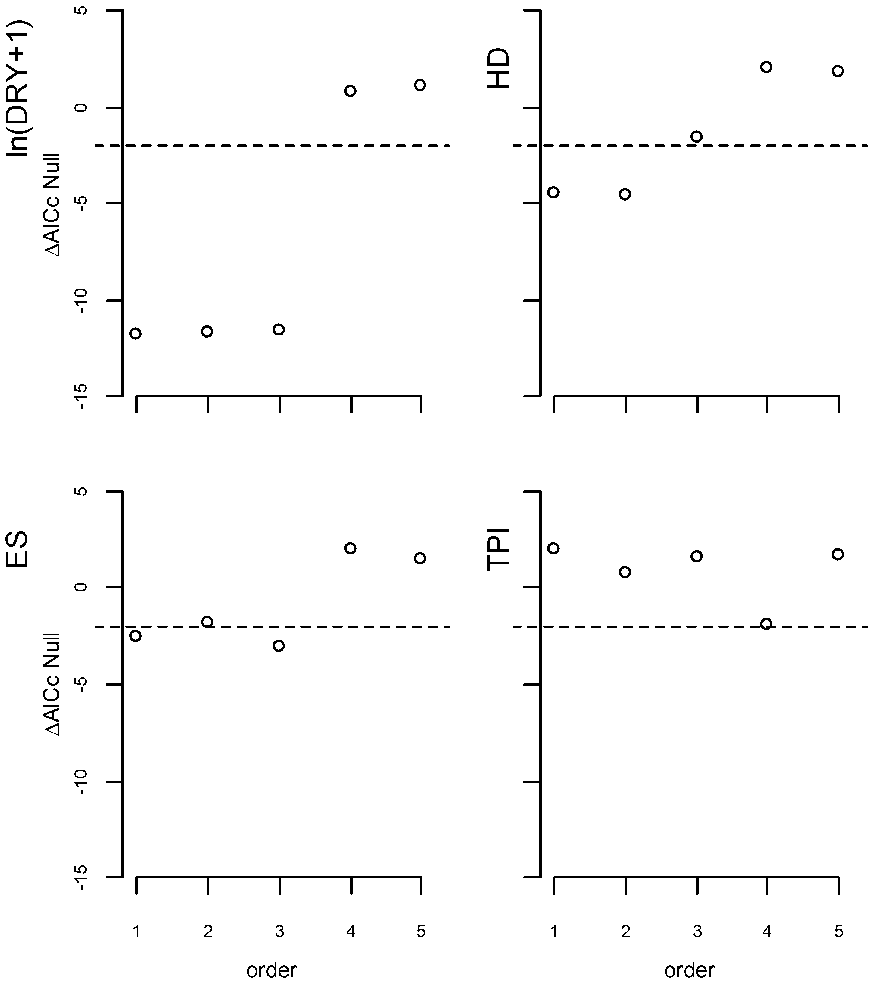
| 1. | Univariate survival models | Figure 5 |
| 2. | Selection of variable scales (ΔAICcNull < 2) | Figure 5 |
| 3. | Removal of correlated variable scales | - |
| 4. | Modeling all possible combinations of variables and scales | - |
| 5. | Analysis of variable scales contributions using model averaging | Table 3 |
| 6. | Selection of the model used for FC prediction based on: | Table A1 |
| (a) ΔAICc | ||
| (b) Simplicity criteria (number of variable-scales involved) | ||
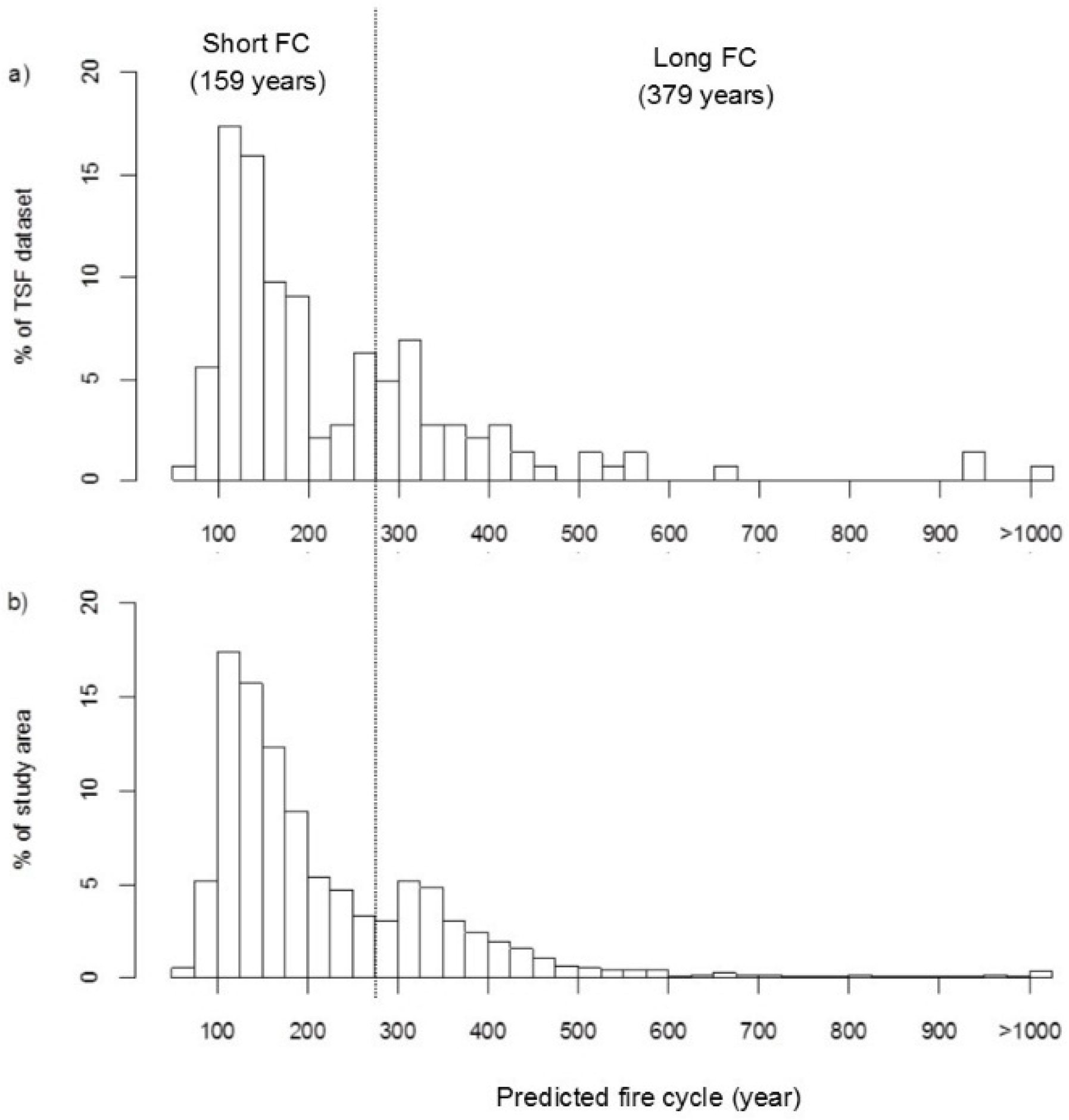
| 7. | Projection of FC for the whole study area | Figure 6 |
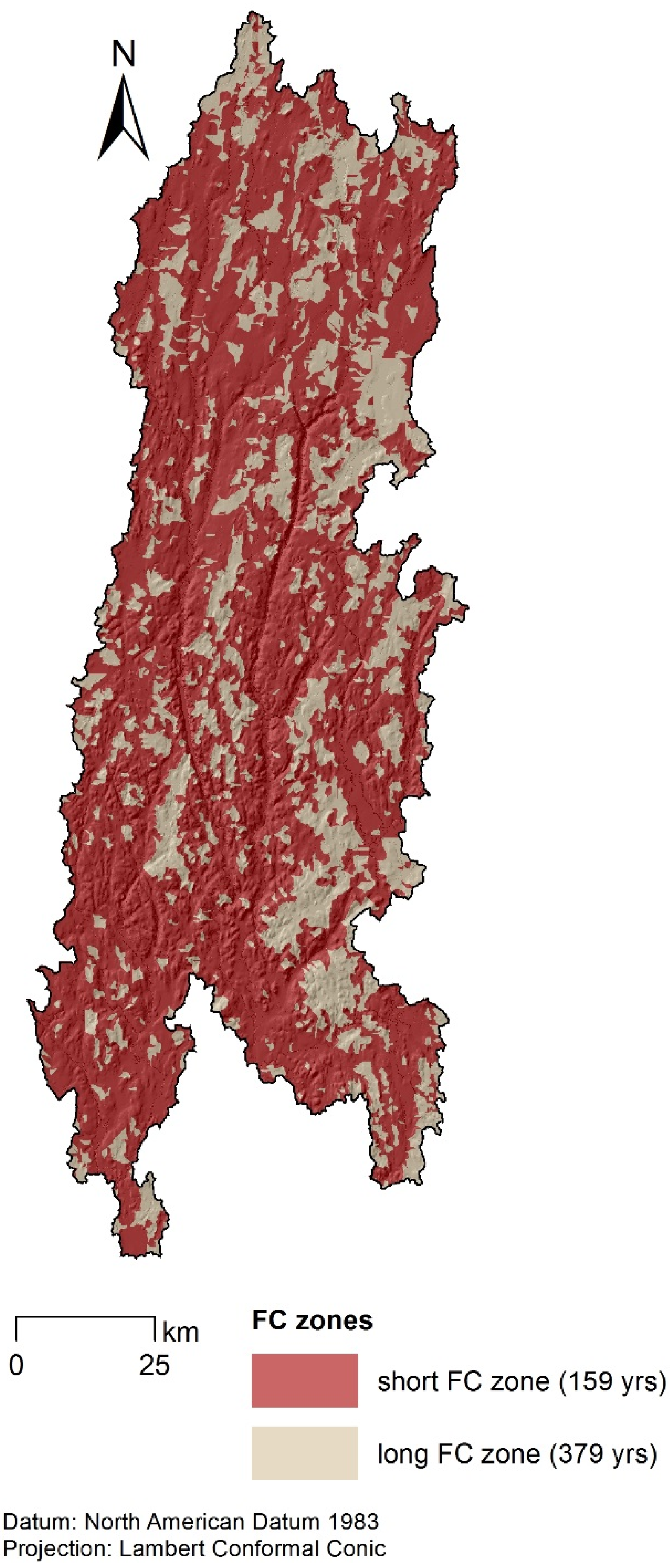
| 8. | Classification of the study area according to FC zones | Table 5, Figure 7 |
| 9. | Validation with independent vegetation data | Table 6 |
| Explanatory Variables | Watershed Order | Relative Importance (Cumulated Weight) | Model-Averaged Estimate | 95% Confidence Interval | |
|---|---|---|---|---|---|
| Lower | Upper | ||||
| ln(DRY + 1) | 1 | 0.73 | 0.1940 | −0.0073 | 0.5097 |
| 3 | 0.68 | 0.2789 | −0.0315 | 0.7927 | |
| HD | 1 | 0.83 | −0.0337 | −0.0830 | −0.0020 |
| 3 | 0.32 | −0.0043 | −0.1039 | 0.0471 | |
| ESD | 1 | 0.45 | 0.0026 | −0.0029 | 0.0143 |
| 3 | 0.38 | 0.0014 | −0.0038 | 0.0109 | |
| TRI | 4 | 0.36 | −0.0426 | −0.3868 | 0.0543 |
| Coefficients | CI (2.5%) | CI (97.5%) | z | Pr (>|z|) | |
|---|---|---|---|---|---|
| ln(DRY + 1)1 | 0.355 | 0.170 | 0.546 | 3.798 | 0.000146 |
| HD1 | −0.0430 | −0.0827 | −0.0154 | −2.510 | 0.012063 |
| ∆AICc | 0.66 | ||||
| n | FC | CI (2.5%) | CI (97.5%) | |
|---|---|---|---|---|
| Short | 100 | 159 | 126 | 198 |
| Long | 44 | 379 | 238 | 590 |
| (a) | Predicted FC (Year) | Forest Age | ||
| Young | Unknown | Old-Growth | ||
| Short (159) | 16 301 (+11.8%) | 19 874 (−5.6%) | 6575 (−8.1%) | |
| Long (379) | 4 093 (−21.2%) | 8 544 (+8.8%) | 3389 (+12.2%) | |
| X2 = 873.5 | p < 0.001 | |||
| df = 2 | Critical distance = 13.82 | |||
| (b) | Predicted FC (Year) | Young Forest Composition | ||
| Black Spruce | Broadleaf | Jack Pine | ||
| Short (159) | 2864 (−1.9%) | 609 (+1.6%) | 1408 (+3.4%) | |
| Long (379 year) | 555 (+11.2%) | 93 (−9.2%) | 186 (−20.0%) | |
| X2 = 19.33 | p < 0.001 | |||
| df = 2 | Critical distance = 13.82 | |||
© 2016 by the authors; licensee MDPI, Basel, Switzerland. This article is an open access article distributed under the terms and conditions of the Creative Commons Attribution (CC-BY) license (http://creativecommons.org/licenses/by/4.0/).
Share and Cite
Bélisle, A.C.; Leduc, A.; Gauthier, S.; Desrochers, M.; Mansuy, N.; Morin, H.; Bergeron, Y. Detecting Local Drivers of Fire Cycle Heterogeneity in Boreal Forests: A Scale Issue. Forests 2016, 7, 139. https://doi.org/10.3390/f7070139
Bélisle AC, Leduc A, Gauthier S, Desrochers M, Mansuy N, Morin H, Bergeron Y. Detecting Local Drivers of Fire Cycle Heterogeneity in Boreal Forests: A Scale Issue. Forests. 2016; 7(7):139. https://doi.org/10.3390/f7070139
Chicago/Turabian StyleBélisle, Annie Claude, Alain Leduc, Sylvie Gauthier, Mélanie Desrochers, Nicolas Mansuy, Hubert Morin, and Yves Bergeron. 2016. "Detecting Local Drivers of Fire Cycle Heterogeneity in Boreal Forests: A Scale Issue" Forests 7, no. 7: 139. https://doi.org/10.3390/f7070139
APA StyleBélisle, A. C., Leduc, A., Gauthier, S., Desrochers, M., Mansuy, N., Morin, H., & Bergeron, Y. (2016). Detecting Local Drivers of Fire Cycle Heterogeneity in Boreal Forests: A Scale Issue. Forests, 7(7), 139. https://doi.org/10.3390/f7070139