Article

The Impact of the Comprehensive Rural Village Development Program on Rural Sustainability in Korea

1
Regional Innovation Research Center for Ocean & Fisheries (RICOF), Korea Maritime Institute, Busan 49111, Korea
2
Department of Agricultural Economics and Rural Development, Seoul National University, Seoul 08826, Korea
*
Author to whom correspondence should be addressed.
Sustainability 2018, 10(7), 2436; https://doi.org/10.3390/su10072436
Submission received: 21 May 2018 / Revised: 2 July 2018 / Accepted: 5 July 2018 / Published: 12 July 2018

Abstract

:
An imperative challenge emerges from the demand to apply the scientific method in the assessment of recent agricultural and rural policies throughout the world. The objective of the present study was to conduct an ex-post quantitative evaluation of the Comprehensive Rural Village Development Program (CRVDP), a representative rural development policy operated by the Ministry of Agriculture, Food and Rural Affairs, a central government agency in South Korea. The primary purpose of this program is to ensure sustainable rural society. This study found a moderate but significant positive impact of the policy in enhancing the standard of living in rural areas. The present paper concludes with suggesting some policy implications, limitations and future directions of policy evaluation studies.

1. Introduction

The rapid economic development in South Korea (hereafter “Korea”) over the past six decades has been deservedly hailed as globally unmatched. Concomitant with this national economic growth has come an increase in both agricultural production and farmer’s income. However, the rural and agricultural environment in Korea has undergone rapid change over the past fifty years. In particular, the trend toward urbanization, which has been accelerating since the mid-1970s, has resulted in decreasing relative competitiveness of agricultural land use in Korea’s rural areas, which today suffer disproportionately from such problems as an aging population, the collapse of basic industries and a lack of social overhead capital, which adversely affect the living conditions of rural residents.
In response, the Korean government has implemented a number of initiatives to revitalize rural areas and to guarantee a sustainable rural society. The initiatives could be a necessary and legitimate redress of the historical siphoning of wealth from rural areas to urban areas. The initiatives by diverse levels of government are key factors to revitalize rural economy for both developed and developing countries [1]. Even so, there is growing concern rooted in changes in popular opinion regarding the massive government investment in resolving such rural problems. Some critics insist that there is a moral hazard in expanding government support for rural residents. However, assigning and assessing values that are associated with such investment involve investigating how the program has affected the values and philosophies constituting Korean society. At the very least, social demand that policy be improved in the interests of promoting greater efficiency and competitiveness in rural areas has increased.
As is well known, policy evaluation can facilitate more successful policy development through a feedback process. With this in mind, the Korean government implemented diverse policy evaluation instruments to improve the overall effectiveness of government policies with regard to rural revitalization and sustainability. However, few studies have been conducted that draw extensively from and inquire deeply into the implications offered by quantitative schema. Moreover, in the case of rural policies, policymakers place more emphasis on policymaking itself than on its objective evaluation. As a result, very few assessments use objective and quantitative techniques to evaluate the impacts of policy, and, in turn, the lack of such evaluation has undermined the credibility of existing assessments, consequently lowering the level of public confidence in policies produced by the Korean government.
The objective of the present study is to conduct an ex-post quantitative evaluation of a representative rural development program operated by the central government in Korea. This study selects a rural development program called the “Comprehensive Rural Village Development Program” (CRVDP) as a subject for an objective evaluation of the impact of rural policies in Korea. The main objective of the CRVDP is to ensure the sustainability of rural society by establishing forward-looking rural communities in which living conditions and livelihoods are in harmony by intensively supporting several key villages in a eup/myeon-unit rural area. The eup/myeon-unit is the lowest level of administrative unit in Korea. The present study constructed a three-step econometrics model incorporating a factor analysis, a spatial econometrics model and a decomposition model, to evaluate the impact of the rural development program on rural sustainability.
Why does the evaluation of values from the CRVDP have to be conducted using a quantitative approach to an ex-post design? By clarifying the factors of success or failure and then analyzing the sustainability of outputs and impacts through objective and retrospective perspective, the evaluation results are able to provide implications for policy-making processes in the future. In addition, this evaluation not only examines the newly formulated policy paradigm for agricultural and rural development but also contributes to balanced urban–rural development policies and social cohesion in Korea from a long-term perspective.
The present study was primarily concerned with formulating a robust quantitative evaluation of the impacts of government policies in rural areas to help resolve the debate and inform continued planning for rural revitalization policies. The remainder of the paper proceeds as follows. Section 2 presents the background of this study. Section 3 addresses and explains relevant methodologies. Section 4 discusses the data and variables taken into account. Section 5 demonstrates the statistical results of this study. Section 6 summarizes our findings and outlines the limitations and policy implications of this study.

2. Rural Policies and Evaluation in Korea

2.1. The Evaluation of Rural Policies

The current rural policy discourse has converted into a viewpoint that emphasizes the spatial value of rural areas by putting rural areas on a par with the agricultural sector [2,3,4]. This policy also transforms functions of the space from rural areas that are limited to food production to areas that attract experience- and leisure-oriented external consumers. However, although the increase in governmental investment can be justified by the multi-functionality of rural places, the limited budget and duality of rural policies require an objective and ex-post evaluation of the agricultural and rural policies [5,6,7]. (Lee and Yun [5] suggested that rural policy has a duality in matching the financial resource providers and the direct beneficiaries of the policy, especially from the urban–rural dichotomous perception.) In addition, when policy effects are demonstrated through ex-post policy evaluation, it is possible to consolidate the validity of political investments.
Nevertheless, agricultural and rural policies have been relatively free from rigorous evaluation measurements, with an emphasis on characteristics of the public property of agriculture and rural places. For these reasons, although not incorporated into the policy evaluation process, these characteristics have expanded only the appearance of the policy without verifying the logic and the effectiveness of the policy. Some groups raise the moral hazard problem, distrust the policies [8] and even draw questions about the effectiveness of the policies [9].
While investigating the relationship between government performance and evaluation has a deep research background [10], consideration of evaluation in rural policy is timely and imminent. OECD [11] shows that policy objectives in member countries have focused more on such rural issues as improving rural competitiveness, enhancing human and social capital, developing niche markets for rural goods and services, diversifying economic activities and so on. However, marked differences in the policies among the member countries exist. Exploring the differences of rural development policy between the EU and the US, Shortall and Warner [12] argued that the EU focused more on the social cohesion that underpins rural development policy due to an emphasis on “Europeanization” that can lessen territorial disparities and guarantee cultural diversity, while the US emphasized market competitiveness as a rationale for rural development, perceiving market mechanisms as the primary instruments for achieving equality.
Incorporating a dualistic construct, Bjorkhaug and Richards [13] contrasted the impacts of market-oriented versus market-protected agricultural policy on agricultural diversity to achieve the goal of sustainable rural development. They found that the market-protected regime was better at sustaining such endogenous goals of multifunctional agriculture as preserving rural space and cultural landscape, maintaining farming livelihoods and ensuring food safety. However, the market-protected approach is highly reliant on government subsidies. Two imperative issues related to this reliance on subsidies are the tighter budget constraints and skepticism regarding the effectiveness of stimulus packages for the spatially targeted interventions [14,15,16]. A strong claim to construct a credible scientific schema that enables researchers to evaluate agricultural and rural policies has been presented from a diverse array of academic disciplines [7,17,18,19]. However, identifying the precise impacts on the intended targets is a complex and challenging task.
One popular approach is the application of an ex-ante design [20]. Considerable efforts have been made in constructing such ex-ante economic models as SAM, I/O and CGE for policy evaluation in both the EU and the US [21]. The ex-ante design determines the possible benefits or pitfalls of a policy through diverse simulation mechanisms and attempts to predict the outcomes of intended policy intervention with given assumptions regarding individuals and circumstances. However, the ex-ante design is subjective and predictive in nature and possesses fundamental limitations to compensate for deviances in real empirical settings. Policies that appear promising before implementation often fail to generate expected outputs. Shumway [22] argued that, regardless of the specific technique used, the ex-ante approach often fails to meet the normative standard of scientific societies.
Due to the litany of ill-conceived and costly rural-development policies and initiatives, examples of successful rural policies are quite rare [11]. Olfert and Patridge [15] suggested that development efforts targeting rural areas require rigorous empirical evidence. Winters et al. [23] and Esposti and Sotte [17] urged that higher standards should be imposed for accurate discernment of the conditions under which rural development policies are justified and how they succeed. Despite the existence of a well-constructed body of literature on policy impacts, little attention has been paid to applying ex-post impact studies to agricultural and rural policies.
An imperative challenge emerges from the demand to incorporate an ex-post empirical approach and quantitative methods to recent rural policies. Walker et al. [7] stressed that pure impact or cost-effectiveness evaluations of agricultural and rural policies should be conducted by adopting an ex-post design that can distinguish the effectiveness of the policies. The ex-post approach overcomes the deficiencies of the ex-ante design because the ex-post approach measures the actual impacts of the policy. A well-designed ex-post evaluation can have substantial spillover effects that link concurrent and future impact evaluations of relevant government policies [6,24].

2.2. Experiences in Korea

Korea’s economic success is best characterized as an example of a latecomer’s high growth rate, compressing the longer developmental history of developed countries in the world into a shorter time period. In 1960, Korea had a per capita gross national product of $80 USD a year, a figure placing it on roughly the same level as Ghana and Sudan and a bit behind India. Since that time Korea’s economy has rapidly advanced and is now consistently near the top of global growth charts, with forty years of growth averaging more than 8% a year until the late-1990s, doubling repeatedly in an exponential explosion of economic expansion. With the exception of neighboring Taiwan, this sustained boom has no historical parallel—not even in postwar Japan. The rapid economic development has lifted Korea’s per capita income from one-third the OECD average in the mid-1980s, to the top quarter of OECD members at present [25].
To modernize its economy, Korea adopted an unbalanced industrial growth strategy. Anticipated imbalances soon became apparent in many areas, such as between urban and rural development, large-scale and small-scale businesses and export-oriented and domestic industries. As a result, although the standard of life of the nation’s population increased substantially, the effect of the benefits has been largely concentrated in only a few regions. Because the economic efficiency-focused development model was widely supported, upholding the so-called “growth pole” strategy, preference was given to a few predetermined industrial policies concentrated within specific urban locations.
This urban-centered strategy has resulted in the speedy collapse of traditional rural communities, best reflected in the shrinking population size and deteriorating economic conditions. In 2010, farm households made up approximately 6.3% (~3.1 million individuals) of the total population, far less than a quarter of the 1970 level. In 2010, 35.6% of rural residents were 65 years of age or older, whereas the national average was approximately 11.8%. Agriculture accounted for approximately 26% of Korea’s GDP in 1970, dropping to 2.4% in 2010. In addition, approximately 26% of GDP and 50.4% of the total labor force were accounted for by agriculture in 1970, whereas, in 2010, these figures were 2.4% and 6.6%, respectively. Rural households are having increasing difficulty in maintaining economic parity with urban households, and the gap in income between farm and urban households should be of grave concern to policy makers. The average income of farm households was higher (111%) than that of urban households in 1975, and average farm household income was comparable to that of urban households until the early 1990s. In 2010, however, farm household income was 66.7% of urban household income (all statistics in this paragraph come from the Korean Statistical Information Service [26]). To lessen this disparity, the Korean government introduced diverse rural policies planned and implemented since the early 1990s, when the gap between rural and urban areas was on the rise.
Rural policy in Korea is more inclined toward the European model, although the political, territorial and cultural contexts of the two domains differ markedly from one another. While planners and policy makers recognize the market failures in rural Korea, they seek to construct a policy of market planning that tries to make rural market systems function. (Market planning is well understood in the management science perspective implying the process of analyzing one or more potentially interesting marketplaces to determine how a business can optimally compete in them. Here, the hybrid concept comes mainly from urban planning and regional science perspective (cf. the online journal, Planning & Market, http://www-pam.usc.edu).) This approach incorporates two seemingly contradictory strategies: planned government interventions and a laissez-faire market system. While the policy posits the explicit pursuit of the construction of laissez-faire market systems in rural areas, the strategic contents of the rural policy are more often aligned with those of the Common Agricultural Policy (CAP) of the EU.
In parallel with the developed economies in the OECD countries, rural policy was synonymous with agricultural policy in Korea until the 1990s. In the 1990s, emphasis shifted to structural adjustment to enhance agricultural competitiveness in the global market. Beginning in 1998, the second phase of the structural adjustment plan to strengthen the agricultural sector and rural development was initiated. In 2004, the Korean government launched a comprehensive plan on agriculture and rural communities and established the “Ten-Year Mid and Long-Term Policy Framework on Agriculture and Rural Communities”.
In each phase, massive investments have been made to achieve the specific goals (Table 1), with 42 trillion Korean Won ($47 billion USD) and 45 trillion Korean Won ($37 billion USD) being invested in the first and second phases of the plan, respectively. The third phase will invest 119 trillion Korean Won ($104 billion USD). These expenditures increased the share of the budget set-aside for agriculture in the total national budget to 13–15% during the 1994–2013 fiscal periods, an increase from 9% in 1993. (Part of the reason is the political power of farmers in Korea. Farmers are enormously influential in the legislative and the executive branches of central government, even though their numbers comprise a very small percentage of the total population. Although the percentage is decreasing every year, they still retain political clout that far exceeds their numbers.)
The agricultural and rural policies to revitalize rural societies in Korea have come under harsh criticism. The major concern of the government investment on agricultural policy is rate of return of the policy. Questions have been raised about the effectiveness of the policies [27] and the moral hazard problem, while many distrust the policies [8,28]. The financial effectiveness of agricultural and rural policies is a global concern, too [19,29]. With a huge investment on agricultural development over the past two decades [11,30], policy makers encounter increased skepticism regarding the efficiency of policy interventions in rural areas [16]. Evidence on the effect of vanity projects in rural areas is found throughout the world [2,31].
As one of the best rural development programs targeting the objective of “enhancing the quality of life in rural areas” in the third phase, the CRVDP is by far the largest program in terms of monetary investment at the village-level undertaken in Korea. The program selects hub villages that have the potential to become rural centers, with the expectation that the benefits these hubs gain will spillover to neighboring rural communities. Hub villages can receive government support of 4–7 billion Korean Won (4 to 7 million USD) for three years. Under this program, a total of 290 hub villages were selected by 2009, with plans to increase the number of hub villages to 1000 by 2017.
While the rural development policy in the third phase constructs a broader set of goals, the CRVDP is based on clear objectives. The four specific objectives of the program are enhancement of farmers’ income, improvement of the residential environment, improving accessibility, and modernization of housing facilities. The investment portfolio of each CRVDP proposed by each local autonomy should be allocated to meet criteria of the four objectives [32]. Before 2010, the CRVDP was designed and initiated at the central government level; however, since then. it has been implemented at lower levels, typically by the local autonomy, that is, the county and some cities encompassing rural areas. While government intervention to resolve rural problems in Korea is warranted, evaluating government policies toward rural development for their effectiveness remains imperative. The following section proposes a methodology for modeling the effectiveness of the rural policy, which, we believe, is immediately transferrable to other cases and countries.

3. Methodology

The policy evaluation that policy-making groups expect could include causal analysis of input to output. How can the impacts of a policy be assessed with limited variables? Identifying causal effect through a quasi-experimental method is one possible alternative [33,34]. In this sense, the present study conducts an econometric analysis and simulations between an experimental group and a comparison group by using spatial econometrics model and decomposition method. To clarify the exact implication of the term in this study, this study used “evaluation” to refer only to the ex-post review of the government action. In this study, the evaluation was performed at the program level, but it could also be performed system-wide or by particular project.
This study offers a novel way to evaluate the impact of rural policies on standards of living in rural Korea. The process of evaluating policy impacts can be separated into three steps: (1) establishing policy goals; (2) implementing various actions to fulfill the goals; and (3) estimating the extent of policy impacts. Each step was converted into quantitative steps for our evaluation model. The relationship between the policy steps and the quantitative steps are shown in Figure 1.
In the first step, we identified goals of the CRVDP and converted them into quantitative indicators known as an evaluation index, as suggested by many previous studies [33,35,36,37,38,39,40]. If the policy objectives are too comprehensive to extract explicit indicators explaining the goal, it is recommended that additional work be performed to create a simple and objective index. As explained in the previous section, because the policy goal of the CRVDP targets the four different objectives, construction of a composite index that reflects the policy goal is essential.
A composite index is made up of two or more variables or measures that are highly related to one another theoretically or statistically. Weighting is an important element in constructing the composite index [42]. From among the diverse weighting methods [43], we chose factor analysis because the weightings can be constructed using the data from the current study. This method is appropriate for constructing the composite variables that are linear combinations of the original variables [44,45]. The composite index in this study is most simply described as the weighted averages of various areal characteristics related to the objectives of the CRVDP. The composite index, which is a summary statistic of a set of area variables, can be fairly described as an objective measure of the living environment in rural areas. In a case such as this study, factor analysis is beneficial because it can be used to analyze how multiple variables are interlinked and enables extracting a common index to incorporate all of the variables related to the policy goal.
The next step was to establish a policy impact evaluation model. The present study adopted three types of spatial econometrics models because the basic unit of our data is aggregated by rural areas and dependent upon spatial characteristics. Unawareness of spatial dependence and spatial heterogeneity can produce statistical bias, as suggested by Anselin [46] and LeSage [47]. Lastly, we applied the decomposition method to identify policy effects, as explained by Oaxaca [48] and Blinder [49]. The advantage of this method for evaluating policy impacts is that it can be used to analyze different groups over the same period of time or the same group over different time periods [50].

3.1. Spatial Econometrics Model

In this study, we applied spatial econometrics models to estimate causal relationship between policy goals and the effect of the policy in areas where it is implemented. Anselin [46] noted that applying an ordinary least-square model to spatially aggregated data may introduce statistical bias due to the spatial dependency and/or spatial heterogeneity of error terms. To overcome such statistical bias, Anselin [51] suggested several spatial econometrics models, such as the spatial autoregressive model (SAR), which assumes that observations that are adjacent should reflect a greater degree of spatial dependence than those more distant from each other [47], expressed as:
Y = ϱ W ( Y ) + X   β +   ε , ε   ~   N ( 0 , σ 2 I ) ,
where Y is an n × 1 vector of dependent variables; X represents an n × k matrix of explanatory variables; W represents a spatial weight matrix containing contiguity relations or functions of distance; the scalar ϱ represents a coefficient on the spatially lagged dependent variable; and β denotes a parameter vector estimated from the explanatory variables.
The second model we utilized is the spatial autoregressive error model (SEM), which is based on the assumption that disturbances exhibit spatial dependence and is expressed as:
Y = X   β +   u ,   u = λ Wu +   ε ,   ε   ~   N   ( 0 ,   σ 2 I ) ,
where the scalar λ represents a coefficient of the spatially correlated errors.
The last model we used in this study is the general spatial model (SAC), which includes both a spatial lag term and a spatially correlated error term. This is expressed as:
  Y =   ϱ W ( Y ) + X   β +   u ,   u = λ Wu +   ε ,   ε   ~   N   ( 0 , σ 2 I ) ,
where the W matrix shown in Models (1)–(3) represents the spatial weight matrix, containing contiguity relations or functions of distance. To reflect spatial dependence between adjacent regions, the W matrix may contain regional information, such as latitude and longitude:
W ij = d ij j = 1 n d ij ,
where W is the n × n spatial weight matrix and d ij is the distance between region i and region j.
The correct interpretation of the estimated coefficients in the SAR and SAC models involves a computation of direct, indirect and total effects. These computations were extensively explained by LeSage and Pace (2009), so we do not reiterate these points here. The direct effect characterizes the average impact of a change in the explanatory variables on the dependent variable at the same location, whereas the indirect effect characterizes the average impact of a change in the explanatory variables on the dependent variable in different locations. The total effect represents the sum of the direct and indirect effects.
The SAR model expressed in Equation (1) can be rewritten to its reduced form in Equation (5) through which the direct and indirect effects can be calculated. It should also be noted that the SAC model shares the same direct and spillover effect properties with the SAR model.
Y = ( I ρ W ) 1 X β + ( I ρ W ) 1
The matrix of partial derivatives of the Equation (5) of Y, E(Y) with respect to the k th explanatory variable of X can be calculated by:
[ E ( Y ) x ik E ( Y ) x nk ] = ( I ρ W ) 1 β k
The diagonal elements of Equation (6) represent direct effects, while the off-diagonal elements represent the indirect effects. Accordingly, the direct and indirect effects can be calculated as:
Direct   effect :   y i x ik = S k ( W ) ii Indirect   effect :   y i x ik = S k ( W ) ji ,   i j ,
where S k ( W ) = ( I ρ W ) 1 β k acting as a “multiplier” matrix that applies higher-order neighboring relations to X k .

3.2. Decomposition Method

Identifying the underlying causes of group and area differences has been the focus of a large amount of research in diverse social-science fields since Blinder [49] and Oaxaca [48] first published their seminal papers four decades ago. For example, Fairlie [50] noted that, “Attesting to the wide use of the Blinder-Oaxaca decomposition technique, more than 1000 citations to these two articles were found in the Social Science Citation Index.” The technique is especially useful for quantifying the different contributions of group differences in factors such as education, experience, marital status and location, as well as group and area gaps in outcomes. The technique is also useful for identifying the causes of geographical, temporal or other categorical differences in outcomes [50]. The decomposition method can be presented formally as follows.
For simplicity, we use Equation (1), but exclude the weight matrix W and the error term, as an example for applying the decomposition method. To identify the net policy impact evaluation using the decomposition method, Equation (1) is divided into two separate equations, as shown below.
Group   ( A ) : E ( Y A ) = j = 1 k β j A X ¯ j A
  Group   ( B ) : E ( Y B ) = j = 1 k β j B X ¯ j B
In a cross-sectional analysis, as shown in Figure 2, Equation (8) applies to the area (A) where the policy has been implemented (treatment group) and Equation (9) applies to the area (B) where the policy has not been implemented (control group). Because Equations (8) and (9) are defined as forms of the expected value, the expected difference between two groups can be directly compared. The theoretical background of the comparison is based on determining the difference between “Do Something” and “Do Nothing”; however, in this study, the estimation of the policy effect contains pair-wise counterfactual simulations beyond the one-dimensional comparison. This estimation is mathematically explained as follows:
The left-hand side of Equation (10) denotes the difference in the policy impact between Group (a) and Group (b). The first part of the right-hand side of Equation (11) is the effect that is explained by the difference in independent variables between two groups, known as the endowment effect. The second part of this formula is the residual effect, which is not clarified by the endowment effect. The total effect is the summation of the endowment and residual effects. Equation (11) shows that the residual effect can be separated into the constant effect and the coefficient effect, where the constant effect represents a direct effect because it indicates the difference between policy implementation and non-implementation, which is not described by effects of independent variables, while the coefficient effect, in contrast, is regarded as an indirect effect. This effect implies what is explained by the difference in the influence of independent variables between the two groups. (It is possible that residual effect may contain unintentional but side–side effects of any potentially important variables other than the effect of CRVDP such as accessibility conditions, industrial structure and other policy impacts. However, the problem of the omitted variables is empirical, and there is little empirical evidence about the error rates when using the Korean Agricultural Census to model the effect of the CRVDP. The limitation is equally applied to other empirical studies that apply the decomposition method [50,52,53].) From a cross-sectional perspective, the treatment group is policy-implemented areas in 2010 and the control group is non-implemented areas in 2010.
E ( Y A ) E ( Y B ) = j = 1 k β j A X ¯ j A     j = 1 k β j B X ¯ j B
= j = 1 k β j A ( X ¯ j A X ¯ j B ) +   j = 1 k X ¯ j B ( β j A β j B )
= j = 1 k β j A ( X ¯ j A X ¯ j B ) + ( β 1 A β 1 B ) + j = 2 k X ¯ j B ( β j A β j B )
Results of applying decomposition methods are represented as forms of simulated effects, such as the endowment, constant and coefficient effects, the results from which policy impacts can be evaluated. At first, the endowment effect increases with the differences in independent variables between two groups in the same time period. In addition, independent variables for assessing policy impacts may consist of variables such as social, demographic or spatial characteristics, which are not directly related to policy impacts. Therefore, the endowment effect should be excluded when evaluating policy impacts.
The residual effect, on the other hand, indicates that the difference in the policy effect occurs as a result of factors other than the difference in the independent variables between two groups over the same time period. Thus, net policy impacts are only evaluated by residual effect not controlled in Equations (8) or (9). As mentioned above, it is differentiated into a constant effect and a coefficient effect. Combinations of each of the effects can be diverse and may result in the following three cases: Case (1), when signs of both the constant and coefficient effects are positive, which implies that the overall policy impact is positive; Case (2), when signs of both the constant and coefficient effects are negative, implying that the overall policy impact is negative; and Case (3), when one effect is positive and the other negative, in which case the overall policy impact is judged by the total effect (the sum of the two effects).

4. Data and Variables

The main purpose of the CRVDP is to establish sustainable rural communities in which the living environment and income are in harmony by intensively supporting key villages of a eup/myeon-unit rural area. The myeon is the lowest administrative unit and where the local administration office is located in Korea. Along with the eup, a myeon is one of the sub-divisions of a county and some cities with a population less than 500,000. A myeon has a smaller population (about 3000–6000 people) than a eup (approximately 20,000 people) and represents the rural areas of a county. Applications of the CRVDP have mainly been focused on myeon areas. Designed by the central government, the initial CRVDP was implemented in 290 eup/myeon units (treatment group) during the period of 2004–2009. (Although the program maintains its original goals, project periods and government investments in the program have been changed since 2010. Now, with financial support from the central government, the program is mainly designed and operated by the local autonomy that enables the local government to be “more accountable and responsive” to the local demand [54].) Because Korea had 1388 eup/myeon administrative units in 2010, the remaining 1098 units are classified as the non-implemented areas (control group). To evaluate the impact of the CRVDP on improving residential environments at the eup/myeon level, data about the administrative units is required. Utilizing the 2010 Agricultural Census Data from Statistics Korea, we constructed aggregated data from the 1388 eup/myeon administrative units, from which we identified 290 units where at least one CRVDP had been implemented between 2004 and 2009.
Table 2 presents variables for analyzing the impacts of the CRVDP as represented by Equations (1)–(3). (We tried to construct as many aggregated independent variables as possible from the census data avoiding the endogenous problem. The statistical problem may arise from our dependent variable (composite index) that was created from the same data with the application of 12 independent variables in factor analysis.) The dependent variable (FACT) was derived by factor analysis. As discussed before, the goals of the CRVDP to enhance standard of living is composed of four primary categories: income enhancement, improvement of the residential environment, improving accessibility and modernization of housing facilities. The dependent variable derived from the factor analysis was designed to reflect these four characteristics, incorporating 12 area characteristics. As the results derived from the factor analysis are not the core focus of the present study, their outputs are listed in Appendix A. The dependent variable should be positively associated with the standard of living in an area; that is, a higher value is indicative of a higher standard of living for a given rural area.
We selected the probable determinants of living standards in rural areas based on the literature and on information available in the census. Because the population of an area may reflect its attractiveness and economy of scale [55,56], we expect that larger populations (POP) in a given rural area are indicative of a higher standard of living in the area. The aging population prevalent in rural areas may lead to negative impacts on community organization and sustainability, such as school closures or consolidations, inter-local cooperation, sharing of administrative functions and so forth [57,58]. Thus, the proportion of elderly people (OLD) may be negatively associated with the level of living conditions in a given rural area. Agriculture is a major source of economic capital in rural areas [59], and its role as an enduring emblem of rural areas is still evident in most developed economies [2,60]. Thus, the proportion of the number of farmers (FARM) should be positively correlated to a better living environment in an area.
Agricultural land is a major economic asset in rural areas [61], and an increase in agricultural land is assumed to result in a rise in the agricultural production of an area [62]. Thus, we expect that the larger the proportion of farmland (AGLAND), the better the economic environment of the area. Agricultural productivity represented by total agricultural sales (AGSALES) in a rural area is directly related to the level of gentrification in the area [56,63], so standard of living in an area should be positively associated with this independent variable. Farm type is an important determinant to obtain agricultural income [62,63] and agricultural income is, on average, high for such crops as vegetables, upland crops (Type 1) and fruit and special crops and flowers (Type 2) in Korea [4,41]. Thus, the standard of living in a rural area is much higher for areas where the majority of farmers cultivate profitable crops than in areas where farmers predominately grow non-profitable crops, such as rice. Among the diverse construction schema of weight matrixes for our spatial econometrics analysis, we apply an inverse distance structure (W) among spatial units that best matched our data characteristics.

5. Results

5.1. Regression Results

To apply spatial econometrics models with statistical validity, a spatial autocorrelation test should be carried out beforehand. We chose to use Moran’s I statistic for our spatial data [64]. The results of Moran’s I indicated that there is spatial dependency in our data at a 99% or higher level, as shown in Table 3. Based on the results of the Moran’s I analysis, regression analyses for the three spatial econometric models explained in Equations (1)–(3) were conducted, the results of which are presented in Appendix B.
Table A5 and Table A6 in Appendix B list the results of the regression analysis of the three econometrics models for the policy implemented areas and the non-implemented areas, respectively. The results show that both the hypothesis of no spatially lagged dependent variable and the hypothesis of no spatially autocorrelated error term should be rejected at the highest significance level at p < 0.01. The results of a spatially lagged dependent variable and a spatially autocorrelated disturbance prove to be statistically significant effects in all three econometrics models for both areas. SAR and SEM show statistically significant effects for the spatially lagged dependent variable (rho) and the spatially autocorrelated disturbance (lambda) and both spatial dependency variables are statistically significant in the SAC model. The explanatory power is slightly higher in the models of the policy implemented area (55–66%) than those of the non-implemented area (36–46%). Among the three spatial econometrics models, SAC displays the highest explanatory power ( R ¯ 2 = adjusted R2) (cf. Appendix B). Therefore, we decide to use the SAC model in the application of the decomposition method for evaluating the CRVDP.
Table 4 presents the estimation results of the SAC model for both areas. The explanatory powers of two areas represented by the adjusted R-squares are 0.46 for the implemented-areas and 0.66 for the non-implemented areas. Considering the cross-sectional characteristics of our data with eight degrees of freedom, the explanatory power of both areas is acceptable for the investigation of individual parameters. The application of the SAC model reveals some interesting results with regard to the determinants of the standard of living in an area, not all of which were expected a priori.
If other factors are held constant, the proportion of population (POP) was found to be positively associated with the standard of living in 1995 (p < 0.01) for both areas. The elasticity of living standard in an area with respect to population is 0.11–0.12, implying that a 1% increase in population is expected to increase the average living standard in an area by 0.11–0.12%. This suggests that rural areas that are more susceptible to urbanization encroachment may offer a better living environment. As expected, the presence of a large elderly population (OLD) in a given rural area is negatively correlated with the level of living standards in both areas. A 1% increase in the number of elderly results in a 0.3% decrease in living standard in the policy non-implemented areas at p < 0.1. However, the effect is much weaker (0.02%) for the policy implemented area with no statistical significance. We suspect that, during the past few decades, aging structure has changed dramatically due to out-migration of younger age groups in the policy implemented areas. This results in the prevailing abundance of elderly people in the policy implemented area. Proportion of farmers (FARM) markedly differs between the two areas. The independent variable is negatively associated with the living standard in the policy implemented area, although this relationship is not significantly different from zero. The reverse is true for the policy non-implemented area, with the highest significance level at p < 0.01. This implies that individual farmers’ contributions to enhancing living standard in an area is much greater in the policy non-implemented area than in the policy implemented area.
Agricultural sales (AGSALE), which represent agricultural productivity in rural area, are positively associated with living standard in the policy non-implemented area, but this effect is not significant in the policy implemented area. Rate of return of agricultural sales to the living standard is twice as large in the implemented area (4.1%) than in the non-implemented area (2.1%). This implies that agriculture is a major economic driver in most rural areas, although agricultural activity is not an enduring emblem for the poorer rural areas in Korea. As expected, the larger is the proportion of farmland (AGLAND) in rural areas, the better is the living standard of the area. This may suggest that agricultural land is functioning as an economic asset in both areas and the elasticity value suggests that a 1% increase in the farmland will enhance the living standard of an area by 0.24% for the policy implemented area and 0.17% for the non-implemented area.
The rate of return by crop to our dependent variable, standard of living in an area, showed the expected effects. The greater the cultivation of such crops as vegetables or upland crops (TYPE1) and fruit, special crops or flower (TYPE 2), the bigger the rate of return for the crops. A 1% increase with respect to the vegetables and upland crops results in a 0.05% increase of the living standard in the policy non-implemented area. The rate of return for the crop in the policy implemented area is slightly higher (0.07%) than in the non-implemented area. The estimates for both independent variables are statistically significant for the policy non-implemented area at p < 0.05 or higher. However, the effect is significantly different from zero for only the vegetables and upland crops in the policy implemented area at a marginal level, p < 0.10.
While some independent variables show similar patterns with respect to our dependent variable, other variables display significant differences between the two areas. To identify differences in the effects of each independent variable on the living standard between areas, we carried out the Wald test, assuming no covariance between the independent variables as shown below:
Wald   Test :   W = ( β i Implemented   β i Not implemented ) 2 ( s . e . ( β i Implemented ) ) 2 + ( s . e . ( β i Not implemented ) ) 2   ~   χ 2   ( 1 )
We identified two independent variables (proportion of elderly people and proportion of farmers) that were significantly different between the two areas. The effect of an aging population on living standard in the policy implemented area was negative and statistically significant, whereas no significant difference was detected in the non-implemented area. As mentioned previously, farmers’ contribution to enhancing living standards in an area was much higher in the policy non-implemented area than in the policy implemented area; that is, the relative availability of human capital was also a determining factor for the difference in living standards between the two areas. This finding is consistent with those reported by Agarwal et al. [55], who detected a strong relationship between economic performance and human capital in rural areas. We suspect that it was the impacts of these two independent variables that influenced the differential living standards between the two areas.
As mentioned before, the direct effect measures how a change in an independent variable in rural area i affects the dependent variable in the area, including feedback effects. The feedback effects occur as a result of impacts rippling through neighboring rural areas and then returning back to the original area. Indirect effects—also called spillover effects—compute the average impact of a change in an independent variable in area i on the dependent variable in all other different locations j. Direct effects are used to test whether a particular variable has a significant effect on the dependent variable within its own geographic area, while indirect effects are used to test whether spillovers into neighboring areas occur [65]. Table 5 presents the results of the direct and indirect effects of independent variables on living standards in rural areas in Korea.
We found that the direct effect estimates have the same signs and similar magnitudes as the point estimates of the independent variables in both areas, as shown in Table 4. Moreover, significance levels for individual parameters in both areas parallel those presented in Table 4, so explanations regarding the independent variables here would be redundant. The feedback effects of the independent variables on living standards in rural areas show a wide range of impacts and are not negligible. For example, the direct effect and the coefficient estimate of the population in the policy implemented area were 0.1409 and 0.1116, respectively, thus the feedback effect is approximately 21%. Other feedback effects range 20–50% in policy implemented areas and 0–17% in the non-implemented areas.
We found that the magnitude of the indirect effects is much larger than their associated direct effects. This may seem counterintuitive, as spillover effects would seem more similar to second-order effects that should be smaller in magnitude than would direct effects. Because the scalar summary measures of the indirect effects provided by [66] combine spatial spillovers in all other areas to produce a single numerical value for the indirect effect estimate, this is not unusual in diverse empirical applications (cf. [26]) particularly if spatial observations are large, as in the present study (1098 + 290 − 1 = 1387).

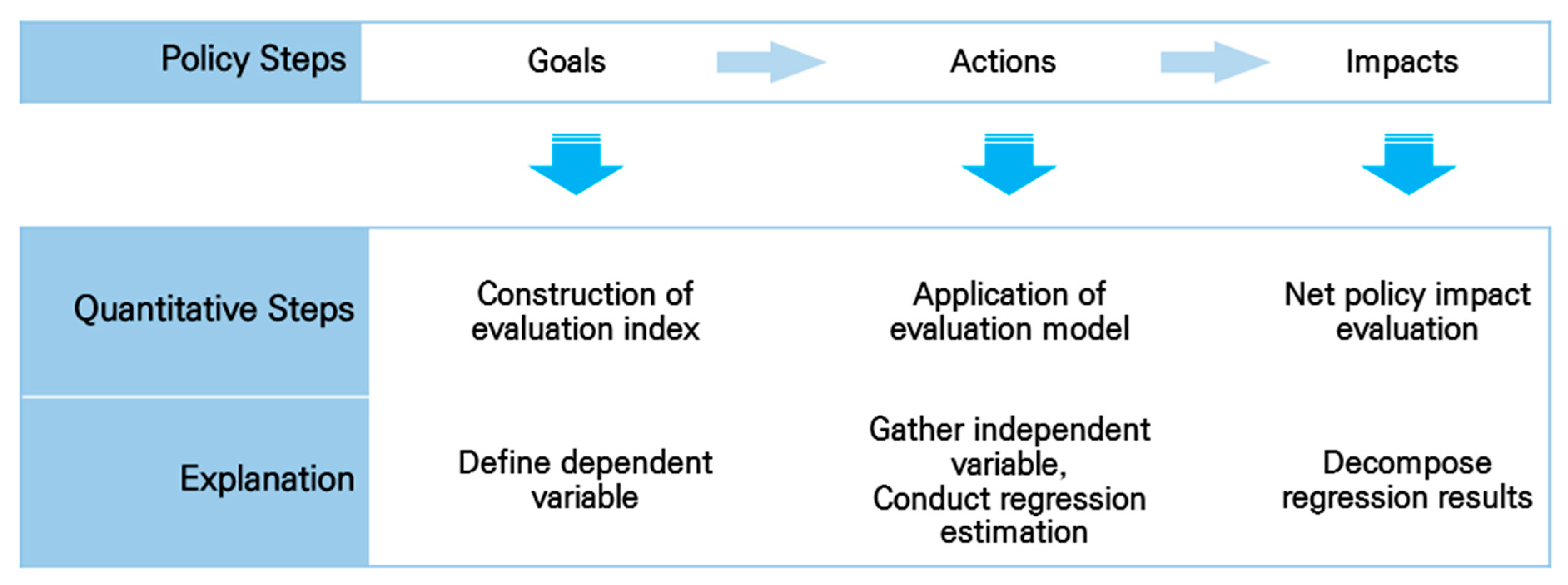
5.2. Decomposition Results

To determine the quantitative implications of the above estimates, the regression results must be simulated to calculate the mean differences of policy implemented and non-implemented areas of the CRVDP, while controlling for spatial characteristics of other independent variables. What is the net effect of mean differences of the policy on the program implemented areas compared with non-implemented areas? What areas where the program had not implemented before would be affected if this program had been enforced? To address these sequential questions, a treatment group should be composed of the areas where the program had been implemented, and a control group should be composed of the areas where the program had not implemented.
We utilize the regression results in 
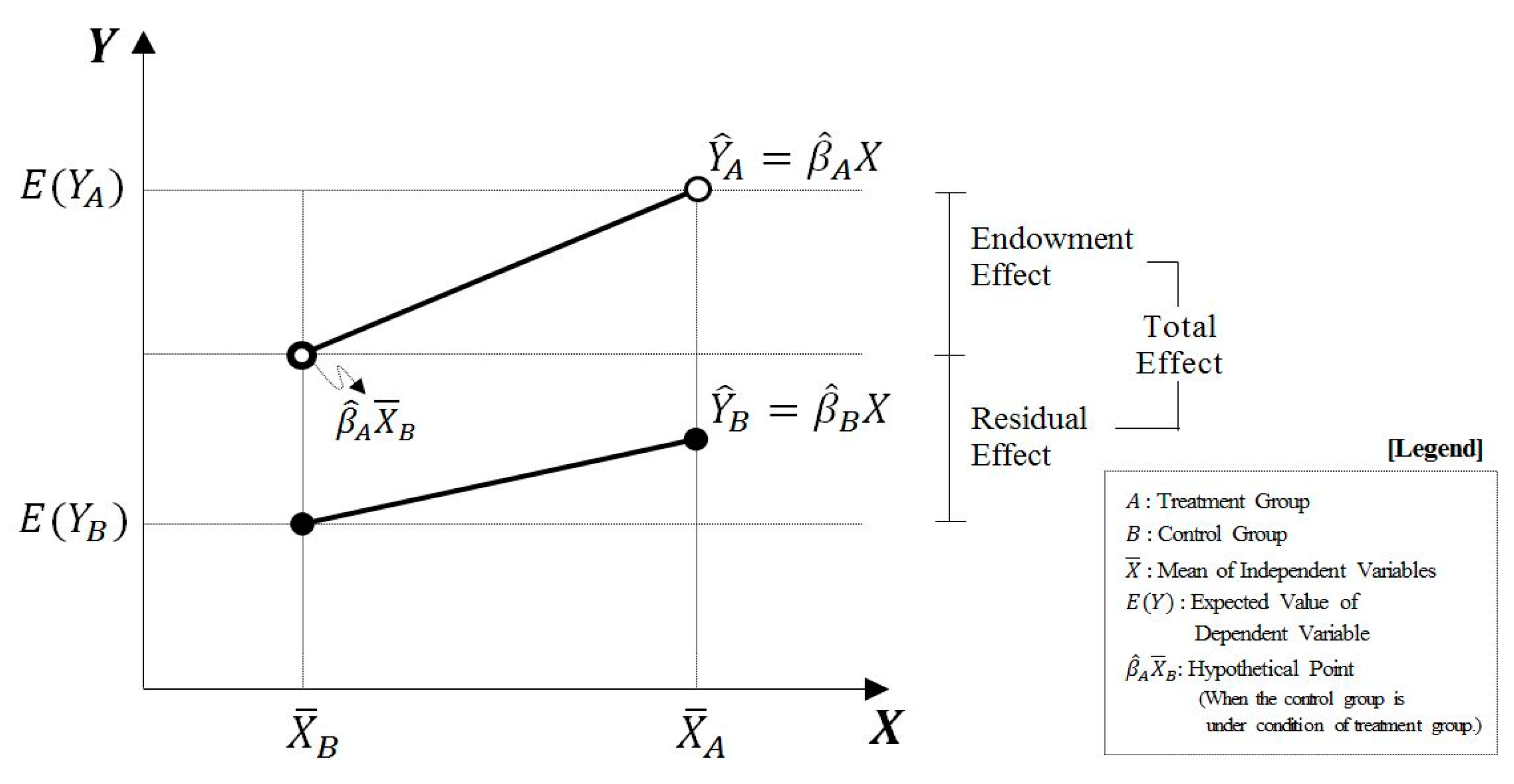
Table 4 to conduct a decomposition method applying Equations (10) and (11), with results presented in Table 6. The results show that the difference between the two areas (0.6320) is composed of the negative endowment effect (−0.0264) and the positive residual effect (0.6584). This implies that the net policy impact calculated after ruling out the endowment effect (which can be explained by the difference of independent variables between the two areas) is 1.04 times as high as the observed impact. That is, the contribution of controlled independent variables in making a better living environment is negative (−4.19%). However, largely due to the uncontrolled policy effect in the residual effect, we can say that the standard of living of the policy impacted areas was enhanced following program implementation; in other words, while the changes in demographics, spatial and agricultural factors in the policy impacted areas are less favorable in producing a better living environment, diverse government policies (such as the CRVDP) intended to enhance living conditions in rural areas have offset the negative changes in the countryside.
The decomposition of residual effects also confirms that the CRVDP has been effective. A constant effect of 0.7987 (126.38%), an average effect contributing to living standards in an area, offset the negative coefficient effect of −0.1403 (−22.19%) to reach the positive residual effect, which implies that the impact of the policy can also be detected indirectly. These positive findings are much clearer when we look more deeply into the composition of individual coefficient effects decomposed from the net effect (refer to Table A7 in Appendix C). In explaining the total endowment effect (−0.0264), demographic variables contributed approximately 92% of total variation, approximately 12.5 times higher explanatory power than that of spatial/agricultural variables. Proportions of population and farmers in an area contributed approximately 89% of total variation of the endowment effect, implying that the major depreciation of the policy implemented area can be explained by these two variables. However, the explanatory power of the spatial/agricultural variables that the CRVDP mainly targets for improvement is approximately 10 times higher (−19.42%) than that of demographic variables (−1.88%). Therefore, the CRVDP can be said to have moderately helped to enhance living conditions in the policy implemented rural areas.

6. Conclusions

Evaluation is the process of valuing beyond philosophical musings [67]. The process determines which values must be included, measures and prioritizes these values and synthesizes the results. Accordingly, assigning and assessing values that are associated with the policy involves examining how the policy has affected the values and philosophies of the society. This study begins to fill the academic and practical vacuum by addressing one primary research question: Does a public policy that has been implemented in rural areas contribute to intended outcomes?
The objective of the present study was to conduct an ex-post quantitative evaluation of the CRVDP, a rural development program operated by the Ministry of Agriculture, Food and Rural Affairs, a central government agency in South Korea. This study conducted an ex-post evaluation of the outcomes after the termination of the program. We constructed a quantitative logic model, which is a stepping-stone to understanding the program and its evaluation mechanisms. The present study conducted an econometric analysis and simulations between policy-implemented areas and non-implemented areas using the spatial econometrics model and the decomposition method. This study found a moderate but significant positive impact of the policy in enhancing the standard of living in rural areas. We found that the CRVDP in Korea represents one of the most significant elements that reflect the recent trend of rural changes from an economy that is based on production to an economy that is based on consumption. We summarize our contributions and findings below.
First, the present study developed a unique means of evaluating the impact of rural policy on rural well-being in Korea, a subject that has largely been overlooked. The proposed process of policy impact evaluation involves three steps, with each step comprising quantitative methods that enable us to interpret the results directly. Second, our aggregated data showed that spatial dependency required correction. The results of the Moran’s I and three spatial econometrics models showed that both the hypothesis of no spatially lagged dependent variable and the hypothesis of no spatially auto-correlated error term should be rejected at p < 0.01 in both areas, which justifies the selection of our econometrics models. Third, this study found that the proportion of the elderly and the proportion of farmers were the most significant differentiating factors between the two areas. We suspect that these two independent variables were primarily responsible for the differences in the standard of living between the two areas. Fourth, the application of the decomposition method revealed, largely due to the uncontrolled policy effect in the residual effect, the standard of living in the program impacted areas has been enhanced following the program implementation.
Based on the results of our analysis, we concluded that the effect of the CRVDP is positive. This result should be an encouraging one for the policymakers who designed the program, and it confirms the important role rural policy can play in improving living conditions in rural areas. Since disparity between urban and rural areas in Korea has been increasing, efforts to reduce poverty in rural areas must continue. While improved access to capital via government subsidies such as the CRVDP can help spark economic vitality in rural areas, rural communities can also use local cultural and historical amenities to shape development strategies. Recently, Korea has successfully promoted some traditionally poor regions as tourist and retirement destinations driven largely by diverse government policies. The Korean government has also initiated policies promoting the more tangible products that emerge from its rural commodities. The incumbent regime in Korea propagates so-called “creative economies” to restructure the national economy and champions the potential of such industries in contributing to rural economic development strategies. However, the lack of a neutral evaluation system may result in deviation from the intended objectives of government policy. Government must therefore be aware that impact evaluations of policies can provide an objective basis for understanding problems and guide future directions for existing policy. Thus, institutionalized establishment of an objective policy evaluation process based on quantitative methods is necessary, as exemplified by a diversity of international agencies [7,23].
Although our study can contribute to the policy evaluation literature, limitations with respect to data and methodologies must be addressed. First, the controlled independent variables to determine living standards in rural areas used in our study show a reasonable value of adjusted R-square in the cross-sectional setting, but more such determinants are needed to increase the explanatory power. Second, the quantitative evaluation method should be corroborated with a schema that can evaluate a pure monetary return of any policy impact. The current ex-post evaluation method with a stochastic property is much more persuasive than other ex-ante or non-stochastic ex-post methods, but this approach could be enhanced by the inclusion of a type of cost–benefit analysis. We believe that further investigations are required to identify monetary value of the policy effect and to distinguish this effect from the aggregate policy effect in the current methodology. Third, in addition to independent variables that are controlled by the quantitative model of the present study, other indicators regarding contextual effects on local and national scopes must be identified because these indicators may also influence the residual effect that this research may fail to capture. Moreover, to develop an evaluation system that covers the transition in rural policy paradigm, various theories and methodologies of the program evaluation must be applied to relevant policies.

Author Contributions

The individual contribution of the authors are as follows: Conceptualization, J.H. and S.L.; Methodology, J.H.; Software, J.P.; Validation, J.H., S.L. and J.P.; Formal Analysis, J.H.; Investigation, J.H.; Resources, J.P.; Data Curation, J.H.; Writing-Original Draft Preparation, J.H.; Writing-Review & Editing, J.H., S.L. and J.P.; Visualization, J.P.; Supervision, S.L.

Funding

This research received no external funding.

Conflicts of Interest

The authors declare no conflict of interest.

Appendix A. Factor Analysis

Variables used for factor analysis to derive an evaluation index (dependent variable) are presented in Table A1. As explained above, the goals of the CRVDP comprise the following four major categories: enhancement of income, betterment of residential environment, improvement of accessibility condition and modernization of housing facilities. The dependent variable derived from the factor analysis is designed to reflect those four major characteristics incorporating a total of 12 area characteristics, as shown in Table A1. Computational processes to construct the evaluation index via the factor analysis is well-known, so we will skip the detailed explanations here. We only provide main outputs of the factor analysis in Table A2, Table A3 and Table A4.
Table A1. Variables for factor analysis.
VariablesExplanation
Income source
   Ratio_salesPercent of farm households that sell agricultural products over 20,000 USD
   Ratio_sidelinePercent of farmers with additional job(s)
   Ratio_comPercent of computer usage
Living environment
   Ratio_waterPercent of water supply
   Ratio_wastePercent of agricultural waste disposal by professional service (or recycling)
   Public_transFrequency of public transportation runs
Accessibility
   Edu_acPercent of existence of formal school education facility
   Bank_acPercent of existence of banking facility (cooperative bank)
   Medi_acPercent of existence of medical facility (public health centre)
Housing condition
   Ratio_kitchenPercent of modernized kitchen
   Ratio_toiletPercent of flush toilets
   Ratio_bathPercent of hot-water boiler
Note. All variables here are continuous. Source: Korea Agricultural Census in 2010, Statistics Korea.
Table A2. MSA values for factor analysis.
VariableRatio_kitchenRatio_toiletRatio_bathRatio_salesRatio_sidelineRatio_comEdu_acBank_acMedi_acRatio_waterRatio_wastePublic_trans
MSA0.76370.73110.66840.45270.70760.45400.73630.71020.75670.75250.77120.7849
Overall MSA (Kaiser’s measure of sampling adequacy) = 0.7006.
Table A3. Eigen values for factor analysis.
FactorEigenvalueProportionCumulative (%)
12.998324.9924.99
22.291819.144.08
31.451912.156.18
41.07088.9265.11
50.92087.6772.78
60.90007.5080.28
70.62355.2085.48
80.50834.2489.71
90.38793.2392.94
100.32712.7395.67
110.27572.3097.97
120.24402.03100.00
Table A4. Standardized factor score and communality estimates.
VariableFactor1Factor2Factor3Factor4Communality
Ratio_sales−0.0401−0.03360.60370.06760.8127
Ratio_sideline0.20250.0882−0.31730.01620.6007
Ratio_com0.11500.07350.4311−0.08230.5016
Ratio_water0.0385−0.02070.05980.57550.6201
Ratio_waste0.1122−0.02530.0574−0.51480.4256
Public_trans0.1152−0.01020.00130.40780.4865
Edu_ac0.03620.3607−0.02500.02590.7983
Bank_ac−0.02810.36350.02240.03220.7820
Medi_ac−0.01370.36470.0068−0.05790.7655
Ratio_kitchen0.2795−0.03870.1005−0.00490.5446
Ratio_toilet0.3279−0.0001−0.0580−0.01290.7401
Ratio_bath0.33970.00270.0543−0.08150.7351
Note 1: Since the evaluation index of this study is the linear sum of factor scores weighted by scoring coefficients, the variables showing negative value are excluded. Note 2: The shadow of the table indicates the group which have similar value.

Appendix B. Regression Results of Spatial Econometrics Models

Table A5. Implemented areas, 2010.
Spatial Econometrics ModelOLS
SARSEMSAC
INTERCEPT−0.2325 5.0038***−6.6532***5.1077***
Demographic variables
POP0.0932***0.0967***0.1116***0.0840***
OLD0.0007 −0.0003 −0.0002 0.0010
FARM−0.0017*−0.0014 −0.0008 −0.0022**
Spatial variables
AGSALE0.0252 0.0263 0.0212 0.0265
AGLAND0.0035***0.0035***0.0024***0.0044***
TYPE10.0006*0.0007*0.0007*0.0006
TYPE20.0001 0.0001 0.0003 −0.0001
Rho0.8770*** 1.9256***
Lambda 0.9440***0.7560***
N290290290290
R20.37120.45430.47580.3980
R ¯ 2 0.35560.44080.46280.3831
Note: * p < 0.1, ** p < 0.05, *** p < 0.01.
Table A6. Non-Implemented areas, 2010.
Spatial Econometrics ModelOLS
SARSEMSAC
INTERCEPT−0.6793***4.9476***−7.4519***5.0536***
Demographic variables
POP0.1045***0.1045***0.1168***0.0980***
OLD−0.0025***−0.0038***−0.0030***−0.0036***
FARM0.0007***0.0008***0.0009***0.0007***
Spatial variables
AGSALE0.0253***0.0377***0.0411***0.0277***
AGLAND0.0032***0.0030***0.0017***0.0038***
TYPE10.0005***0.0005**0.0005***0.0005**
TYPE20.0005**0.0003 0.0005**0.0003
Rho0.9360*** 2.0250***
Lambda 0.9890***2.3409***
N1098109810981098
R20.54760.62670.66350.5943
X ¯ 2 0.54470.62430.66130.5917
Note: * p < 0.1, ** p < 0.05, *** p < 0.01.

Appendix C. Decomposition of Individual Independent Variables

Table A7. Decomposition of individual parameters.
Endowment EffectRatio (%)Residual EffectRatio (%)Total ExplanationRatio (%)
Intercept0.00000.000.7987121.300.7987126.38
Demographic variables
   POP−0.019874.97−0.0431−6.55−0.0629−9.96
   OLD−0.00072.780.087513.290.086813.73
   FARM−0.003714.03−0.0568−8.63−0.0605−9.57
   Sub total−0.024391.79−0.0124−1.88−0.0366−5.80
Spatial variables
   AGSALE0.0004−1.49−0.1433−21.76−0.1429−22.61
   AGLAND−0.003412.700.01191.810.00851.35
   TYPE10.0004−1.370.00580.880.00610.97
   TYPE20.0004−1.62−0.0023−0.35−0.0018−0.29
   Sub total−0.00228.21−0.1279−19.42−0.1300−20.58
Total−0.0264100.000.6584100.000.6320100.00

References

  1. Li, Y.; Westlund, H.; Zhen, X.; Liu, Y. Bottom-up initiatives and revival in the face of rural decline: Case studies from China and Sweden. J. Rural Stud. 2016, 47, 506–513. [Google Scholar] [CrossRef] [Green Version]
  2. Woods, M. Rural Geography; Sage: Thousand Oaks, CA, USA, 2005. [Google Scholar]
  3. Brandth, B.; Haugen, M.S. Farm divesification into tourism-implications for social identity? J. Rural Stud. 2011, 27, 35–44. [Google Scholar] [CrossRef] [Green Version]
  4. Hwang, J.H.; Lee, S.W. The Effect of the Rural Tourism Policy on Non-farm Income in Korea. Tour. Manag. 2015, 46, 501–513. [Google Scholar] [CrossRef]
  5. Lee, S.W.; Yun, S.D. Research Paper: Quantitative Approaches for Agricultural and Rural Policy Evaluation. J. Korea Soc. Rural Plan. 2008, 14, 97–108. [Google Scholar]
  6. Leeuw, F.L.; Vaessen, J. Impact Evaluations and Development: NONIE Guidance on Impact Evaluation; Network of Networks for Impact Evaluation: Washington, DC, USA, 2009. [Google Scholar]
  7. Walker, T.; Ryan, J.; Kelly, T. Impact Assessment of Policy-oriented International Agricultural Research: Evidence and Insights from Case Studies. World Dev. 2010, 38, 1453–1461. [Google Scholar] [CrossRef]
  8. Lee, S.W.; Kim, H.J. Agricultural Transition and Rural Tourism in Korea: Experiences of the Last Forty Years; Asian Institute of Technology: Bangkok, Thailand, 2010. [Google Scholar]
  9. Wang, C.; Xu, H. Government intervention in investment by Chinese listed companies that have diversified into tourism. Tour. Manag. 2011, 32, 1371–1380. [Google Scholar] [CrossRef]
  10. Hoey, L. Show Me the Numbers: Examining the Dynamics between Evaluation and Government Performance in Developing Countries. World Dev. 2015, 70, 1–12. [Google Scholar] [CrossRef]
  11. OECD. Rural Policy Reviews; OECD: Paris, France, 2009. [Google Scholar]
  12. Shortall, S.; Warner, M.E. Social Inclusion or Market Competitiveness? A Comparison of Rural Development Policies in the European Union and the United States. Soc. Policy Adm. 2010, 44, 575–597. [Google Scholar] [CrossRef]
  13. Bjorkhaug, H.; Richards, C.A. Multifunctional Agriculture in Policy and Practice? A Comparative Analysis of Norway and Australia. J. Rural Stud. 2008, 24, 98–111. [Google Scholar] [CrossRef]
  14. Glaeser, E.L.; Gottleib, J.D. The Economics of Place-making Policies. Brook. Pap. Econ. Activ. 2008, 39, 155–239. [Google Scholar] [CrossRef]
  15. Olfert, M.R.; Partridge, M.D. Best Practices in Twenty-first-century Rural Development and Policy. Growth Chang. 2010, 41, 147–164. [Google Scholar] [CrossRef]
  16. World Bank. World Development Report: Reshaping Economic Geography; The World Bank: Washington, DC, USA, 2009. [Google Scholar]
  17. Esposti, R.; Sotte, F. Evaluating the Effectiveness of Agricultural and Rural Policies: An Introduction. Eur. Rev. Agric. Econ. 2013, 40, 535–539. [Google Scholar] [CrossRef]
  18. Hill, B.; Wojan, T.R. Evaluation of Rural Development Policy. EuroChoices 2010, 9, 22–23. [Google Scholar] [CrossRef]
  19. Olfert, M.R.; Partridge, M.D.; Berdegue, J.; Escobal, J.; Jara, B.; Modrego, F. Places for Place-based Policy. Dev. Policy Rev. 2014, 32, 5–32. [Google Scholar] [CrossRef]
  20. Helming, K.; Perez-Soba, M.; Tabbush, P. Suatainability Impact Assessment of Land Use Changes; Springer: Berlin, Germany, 2008. [Google Scholar]
  21. Johnson, T.G.; Roberts, D.; Wojan, T.R. Model-based Evaluation of Rural Development Policies. EuroChoices 2010, 9, 30–36. [Google Scholar] [CrossRef]
  22. Shumway, C.R. Subjectivity in Ex-ante Research Evaluation. Am. J. Agric. Econ. 1980, 63, 169–173. [Google Scholar] [CrossRef]
  23. Winters, P.; Maffioli, A.; Salazar, L. Introduction to the Special Feature: Evaluating the Impact of Agricultural Projects in Developing Countries. J. Agric. Econ. 2011, 62, 393–402. [Google Scholar] [CrossRef]
  24. Khandker, S.R.; Koolwal, G.B.; Samad, H.A. Handbook on Impact Evaluation: Quantitative Methods and Practices; The Word Bank: Washington, DC, USA, 2010. [Google Scholar]
  25. OECD. Economic Policy Reforms 2013: Going for Growth; OECD: Paris, France, 2013. [Google Scholar]
  26. Lacombe, D.; LeSage, J.P. Use and Interpretation of Spatial Autoregressive Probit Models; Springer: Berlin/Heidelberg, Germany, 2013. [Google Scholar]
  27. Lee, S.W.; Nam, S.Y. Agro-Tourism as a Rural Development Strategy in Korea. J. Rural Dev. 2005, 29, 67–83. (In Korean) [Google Scholar]
  28. Lee, H.J. Changes in Rural Policy Paradigm and Rural Development Project in Korea: A Study Based on Integrated Rural Village Development Project. Rural Soc. 2009, 19, 17–47. (In Korean) [Google Scholar]
  29. Ogundari, K. The Paradigm of Agricultural Efficiency and Its Implication on Food Security in Africa: What Does Meta-analysis Reveal? World Dev. 2014, 64, 690–702. [Google Scholar] [CrossRef]
  30. OECD. Evaluation of Agricultural Policy Reforms in Korea; OECD: Paris, France, 2008. [Google Scholar]
  31. Fahrmann, B.; Grajewski, R. How Expensive is the Implementation of Rural Development Programmes? Eur. Rev. Agric. Econ. 2013, 40, 541–572. [Google Scholar] [CrossRef]
  32. Ministry of Agriculture, Forestry and Fisheries (MAFF). The White Paper: Comprehensive Rural Village Development Program; MAFF: Seoul, Korea, 2011. (In Korean) [Google Scholar]
  33. Campbell, D.T.; Stanley, J.C. Experimental and Quasi-Experimental Designs for Research on Teaching; Rand McNally: Chicago, IL, USA, 1963. [Google Scholar]
  34. Guba, E.G.; Lincoln, Y.S. Effective Evaluation: Improving the Usefulness of Evaluation Results through Responsive and Naturalistic Approaches; Jossey-Bass: San Francisco, CA, USA, 1981. [Google Scholar]
  35. Au, N.; Hollingsworth, B.; Spinks, J. Measuring the Efficiency of Health Services in Lower-income Countries: The Case of Papua New Guinea. Dev. Policy Rev. 2014, 32, 259–272. [Google Scholar] [CrossRef]
  36. Deninston, O.L.; Rosenstock, L.; Getting, V. Evaluation of Program Effectiveness. Public Health Rep. 1986, 83, 333–334. [Google Scholar]
  37. Hatry, H.; Blair, L.; Fisk, D.; Kimmel, W. Program Analysis for State and Local Government; The Urban Institute: Washington, DC, USA, 1976. [Google Scholar]
  38. Liu, Z.; Lan, J. The Sloping Land Conversion Program in China: Effect on the Livelihood Diversification of Rural Households. World Dev. 2015, 70, 147–161. [Google Scholar] [CrossRef]
  39. Madaus, G.F.; Scriven, M.; Stufflebeam, D.L. Evaluation Models; Viewpoint on Educational and Human Services Evaluation; Kluwer-Nijhoff: New York, NY, USA, 1983. [Google Scholar]
  40. Wholey, J.S. Evaluation: Promise and Performance; The Urban Institute: Washington, DC, USA, 1979. [Google Scholar]
  41. Lee, S.W.; Kim, H.J. The Effects of Rural Settlement Projects on the Living Environment in Korea. Harv. Asia Q. 2011, 13, 6–13. [Google Scholar]
  42. Boldin, M.D. A Critique of the Traditional Composite Index Methodology. J. Econ. Soc. Meas. 1998, 25, 119–140. [Google Scholar]
  43. Dillon, W.R.; Goldstein, M. Multivariate Analysis: Methods and Applications; John Wiley & Sons: New York, NY, USA, 1984. [Google Scholar]
  44. Kaiser, H.F. An Index of Factorial Simplicity. Psychometrika 1974, 39, 31–36. [Google Scholar] [CrossRef]
  45. Sharma, S. Applied Multivariate Techniques; John Wiley & Sons: New York, NY, USA, 1996. [Google Scholar]
  46. Anselin, L. Spatial Econometrics: Methods and Models; Kluwer Academic Press: Philip Drive Norwell, MA, USA, 1988. [Google Scholar]
  47. LeSage, J.P. The Theory and Practice of Spatial Econometrics. 1999. Available online: http://www.econ.utoledo.edu/ (accessed on 1 May 2018).
  48. Oaxaca, R. Male-female Wage Differentials in Urban Labour Markets. Int. Econ. Rev. 1973, 14, 693–709. [Google Scholar] [CrossRef]
  49. Blinder, A.S. Wage Discrimination: Reduced Form and Structural Estimation. J. Hum. Resour. 1973, 5, 436–455. [Google Scholar] [CrossRef]
  50. Fairlie, R.W. An Extension of the Blinder-Oaxaca Decomposition Technique to Logit and Probit Models. J. Econ. Soc. Meas. 2005, 30, 305–316. [Google Scholar]
  51. Anselin, L. Spatial Externalities, Spatial Multipliers, and Spatial Econometrics. Int. Reg. Sci. Rev. 2003, 26, 153–166. [Google Scholar] [CrossRef]
  52. Ault, R.W.; Ekelund, R.B., Jr.; Jackson, J.D.; Saba, R.S.; Saurman, D.S. Smoking and Absenteeism. Appl. Econ. 1991, 23, 743–754. [Google Scholar] [CrossRef]
  53. Wachter, S.M.; Megbolugbe, I.F. Impacts of Housing and Mortgage Market Discrimination on Racial and Ethnic Disparities in Homeownership. Hous. Policy Debate 1992, 3, 332–370. [Google Scholar] [CrossRef]
  54. Faguet, J.P. Decentralization and Governance. World Dev. 2013, 53, 2–13. [Google Scholar] [CrossRef]
  55. Agarwal, S.; Rahman, S.; Errington, A. Measuring the Determinants of Relative Economic Performance of Rural Areas. J. Rural Stud. 2009, 25, 309–321. [Google Scholar] [CrossRef]
  56. Nelson, P.B.; Oberg, A.; Nelson, L. Rural Gentrification and Linked Migration in the United States. J. Rural Stud. 2010, 26, 343–352. [Google Scholar] [CrossRef]
  57. Burholt, V.; Dobbs, C. Research on Rural Ageing: Where We Have Got to and Where are We Going in Europe. J. Rural Stud. 2012, 28, 432–446. [Google Scholar] [CrossRef]
  58. Glasgow, N.; Brown, D.L. Rural Ageing in the United States: Trends and Contexts. J. Rural Stud. 2012, 28, 422–431. [Google Scholar] [CrossRef]
  59. Sanchez-Zamora, P.; Cobos, R.G.; Delgado, F.C. Rural Areas Face the Economic Crisis: Analyzing the Determinants of Successful Territorial Dynamics. J. Rural Stud. 2014, 35, 11–25. [Google Scholar] [CrossRef]
  60. McManus, P.; Walmsley, J.; Argent, N.; Baum, S.; Bourke, L.; Martin, J.; Pritchard, B.; Sorensen, T. Rural Community and Rural Resilience: What is Important to Farmers in Keeping Their Country Towns Alive? J. Rural Stud. 2012, 28, 20–29. [Google Scholar] [CrossRef]
  61. Xie, H. Towards Sustainable Land Use in China: A Collection of Empirical Studies. Sustainability 2017, 9, 2129. [Google Scholar] [CrossRef]
  62. Alasia, A.; Weersink, A.; Bollman, R.D.; Cranfield, J. Off-farm Labour Decision of Canadian Farm Operators: Urbanization Effects and Rural Labour Market Linkages. J. Rural Stud. 2009, 25, 12–24. [Google Scholar] [CrossRef]
  63. Van Leeuwen, E.; Dekkers, J. Determinants of Off-farm Income and Its Local Patterns. A Spatial Microsimulation of Dutch Farmers. J. Rural Stud. 2013, 31, 55–66. [Google Scholar] [CrossRef]
  64. Rogerson, P.A. Statistical Methods for Geography; Sage: Thousand Oaks, CA, USA, 2006. [Google Scholar]
  65. Elhorst, J.P.; Zigova, K. Evidence of Competition in Research Activity among Economic Departments Using Spatial Econometric Techniques; Working Paper Series 2011-04; Department of Economics, University of Konstanz: Konstanz, Germany, 2011. [Google Scholar]
  66. LeSage, J.P.; Kelley, P.R.; Lam, N.; Campanella, R.; Liu, X. New Orleans Business Recovery in the Aftermath of Hurricane Katrina. J. R. Stat. Soc. Ser. A Stat. Soc. 2011, 174, 1007–1027. [Google Scholar] [CrossRef]
  67. Shadish, W.R.; Cook, T.D.; Leviton, L.C. Foundations of Program Evaluation: Theories of Practice; Sage: London, UK, 1991. [Google Scholar]
Figure 1. Relationship between policy steps and quantitative steps (Source: Lee and Kim [41].)
Sustainability 10 02436 g001
Figure 2. Graphical expression of decomposition technique (Source: Hwang and Lee [4]).
Sustainability 10 02436 g002
Table 1. Agricultural and rural investment plans in Korea, 1991 to 2017.
PhasesTitlesPeriodMajor ObjectiveBudget
1′stAgricultural and Rural Structure Improvement Plan1991–1996- Strengthening the competitiveness of the agricultural sector42 Trillion Korean Won (47 Billion USD)
2′ndAgricultural and Rural Structure Adjustment Plan1997–2003- Strengthening the competitiveness of the agricultural sector and rural areas45 Trillion Korean Won (37 Billion USD)
3′rdComprehensive Plan on Agriculture and Rural Communities2004–2017- Development of agri-food sector
- Enhancing the competitiveness of the agricultural sector
- Enhancing the quality of life in rural areas
119 Trillion Korean Won (104 Billion USD)
Table 2. Explanation of variables for spatial econometrics models.
VariablesExplanation
Dependent variable (FACT)Log (factor scores derived from factor analysis)
Demographic independent variables
  POPLog (total population)
  OLDProportion of over 65 aged people (%)
  FARMProportion of farmers (%)
Spatial independent variables
  AGSALELog (average sales of agricultural products) (10 USD)
  AGLANDProportion of farming land (%)
  TYPE1Proportion of vegetable and upland crops (%)
  TYPE2Proportion of fruit, special crop, flower (%)
Spatial lag matrix
   WSpatial weight matrix (inverse distance)
Source: 2010 Agricultural Census, Statistics Korea.
Table 3. Results of Moran’s I.
Implemented AreaNon-Implemented Area
Moran’s Ip-valueMoran’s Ip-value
0.16440.00000.26380.0000
Table 4. Results of spatial econometrics models.
VariablesImplemented AreaNon-Implemented Area|Wald Test|
INTERCEPT−6.6532***−7.4519***
POP0.1116***0.1168***
OLD−0.0002 −0.0030*****
FARM−0.0008 0.0009*****
AGSALE0.0212 0.0411***
AGLAND0.0024***0.0017***
TYPE10.0007*0.0005***
TYPE20.0003 0.0005**
Rho1.9256***2.025***
Lambda0.7560***2.3409***
N2901098
R20.47580.6635
R ¯ 2 0.46280.6613
Note: * p < 0.1, ** p < 0.05, *** p < 0.01. The values in Wald Test are converted to probability.
Table 5. Direct, indirect and total effects from SAC model.
VariablesImplementedNot-Implemented
Direct EffectIndirect EffectTotal EffectDirect EffectIndirect EffectTotal Effect
POP0.1409***6.9629***7.1038***0.1235***7.3411***7.4646***
OLD−0.0003 −0.0155 −0.0158 −0.0031***−0.1836***−0.1867***
FARM−0.0010 −0.0511 −0.0522 0.0010***0.0579***0.0589***
AGSALE0.0257 1.2679 1.2935 0.0435***2.5856***2.6291***
AGLAND0.0030***0.1491***0.1521***0.0018***0.1064***0.1082***
TYPE10.0009*0.0461*0.0470*0.0006***0.033***0.0335***
TYPE20.0004 0.0207 0.0211 0.0005**0.0296**0.0300**
Note: * p < 0.1, ** p < 0.05, *** p < 0.01.
Table 6. Direct, indirect and total effects from SAC model.
AmountRatio (%)Evaluation
Endowment effect−0.0264−4.19Negative
Residual effect: Net effect0.6584104.19Positive
   Constant effect0.7987126.38Positive
   Coefficient effect−0.1403−22.19Negative
Total effect0.6320100.00Positive

