Low Carbon Scheduling Optimization of Flexible Integrated Energy System Considering CVaR and Energy Efficiency

1
School of Management Engineering, Zhengzhou University of Aeronautics, Zhengzhou 450000, China
2
School of Economics and Management, North China Electric Power University, Beijing 102206, China
*
Author to whom correspondence should be addressed.
Sustainability 2019, 11(19), 5375; https://doi.org/10.3390/su11195375
Submission received: 1 September 2019
/
Revised: 16 September 2019
/
Accepted: 25 September 2019
/
Published: 28 September 2019
(This article belongs to the Special Issue Developing Multi-Energy Systems: Technologies, Methods and Models)
Abstract
:With the rapid transformation of energy structures, the Integrated Energy System (IES) has developed rapidly. It can meet the complementary needs of various energy sources such as cold, thermal, and electricity in industrial parks; can realize multi-energy complements and centralized energy supplies; and can further improve the use efficiency of energy. However, with the extensive access of renewable energy, the uncertainty and intermittentness of renewable energy power generation will greatly reduce the use efficiency of renewable energy and the supply flexibility of IES so as to increase the operational risk of the system operator. With the goal of minimum sum of the system-operating cost and the carbon-emission penalty cost, this paper analyzes the combined supply of cooling, heating, and power (CCHP) influence on system efficiency, compared with the traditional IES. The flexible modified IES realizes the decoupling of cooling, thermal, and electricity; enhances the flexibility of the IES in a variety of energy supply; at the same time, improves the use efficiency of multi-energy; and reasonably avoids the occurrence of energy loss and resource waste. With the aim of reducing the risk that the access of renewable energy may bring to the IES, this paper introduces the fuzzy c-mean-clustering comprehensive quality (FCM-CCQ) algorithm, which is a novel method superior to the general clustering method and performs cluster analysis on the output scenarios of wind power and photovoltaic. Meanwhile, conditional value at risk (CVaR) theory is added to control the system operation risk, which is rarely applied in the field of IES optimization. The model is simulated in a numerical example, and the results demonstrate that the availability and applicability of the presented model are verified. In addition, the carbon dioxide emission of the traditional operation mode; thermoelectric decoupling operation mode; and cooling, thermal, and electricity decoupling operation mode of the IES decrease successively. The system flexibility is greatly enhanced, and the energy-use rate of the system is improved as a whole. Finally, IES, after its flexible transformation, significantly achieve energy conservation, emission reduction, and environmental protection.
1. Introduction
1.1. Background and Motivation
With the high-speed development of the economy, fossil energy is increasingly exhausted. Moreover, with the consumption of fossil energy, the emission of greenhouse gases (GHG) leads to the further deterioration of the environment [1]. Economic development will further worsen the environment if emissions of pollutants are not controlled [2]. Countries all over the world are constantly adjusting their energy structure in order to find new energy alternatives. Therefore, the renewable and clean energy dominated by solar energy and wind energy has been widely concerned. It is an irresistible trend for clean energy to replace fossil energy [3]. Meanwhile, the emergence of the concept of multi-energy complementary integrated energy system (IES) provides an effective theoretical basis for the comprehensive use of renewable energy and promotes the consumption of renewable energy [4]. Generally, IES refers to the use of advanced physical information technology and innovative management modes in a certain region and to the integration of regional coal, oil, natural gas, electrical energy, thermal energy and other kinds of energy to achieve a variety of heterogeneous energy subsystems: coordination planning, optimization operation, collaborative management, and interactive and complementary response. IES can meet people’s demand for various energy sources (such as cold energy, thermal energy, and electric energy), so it can also be called an energy hub. In IES, various distributed renewable energy generators, energy storage devices, and auxiliary components constitute a controllable energy system. However, due to the uncertainty and intermittentness of wind power and photovoltaic output, the flexible power supply of IES is decreased. At the same time, considering the existence of gas turbines, the production of heat and electricity in the comprehensive energy system has some degree of interconnection [5], which is often restricted by heat load. This mode of operation is often referred to as “following the thermal load (FTL)”. IES generally adopts this mode to avoid waste of resources. This fixed operational mode has a fatal weakness which greatly reduces the flexibility of IES, so the improvement of the flexibility of IES has further research value and significance [6].
1.2. Literature Review
Previous researches up to now on the flexibility of IES are summarized as follows:
The flexibility of IES can be considered from the energy supply side and energy demand side. On the energy supply side, there is no doubt that natural gas is one of the main energy inputs for most IESs, which can be converted into electricity and thermal and, further, into cold energy. However, as a nonrenewable fossil energy, natural gas will inevitably restrict IES future development. Therefore, numerous researchers began to devote themselves to the conversion technology of other energy sources into natural gas, and Power to Gas (P2G) technology, which can convert surplus electric energy into natural gas (methane) or hydrogen, began to appear in people’s vision [7]. The emergence of P2G technology makes the supply of natural gas more flexible. Instead of relying solely on imports, it can use renewable energy (such as wind, solar, water, etc.) to generate electricity. P2G technology can be used to convert electric energy into natural gas, realizing the mutual conversion and comprehensive use of various energy sources. Reference [8] proposed two different P2G technologies to accomplish the mutual flexible conversion of electricity, which are fully applicable to the future development of IES. A simulation is used to demonstrate that this flexible energy-use mechanism is of great help to improve the economic benefits, environmental benefits, and energy-use efficiency of IES. In addition, the flexibility of the energy supply side corresponds not only to the mutual transformation of various energy sources but also to the diversity of energy use. In Reference [9], the technical scheme design of using geothermal energy for supplying cooling/heating energy is proposed, which obtains better environmental benefits compared with electric heat pump and gas engine heat pump. A solar–biomass hybrid power generation system has been mentioned in Reference [10], which adopts solar and biomass energy to generate electricity, and it provides new ideas for the sustainable use of future energy sources. From the perspective of the energy demand side, it is no doubt that the flexibility of the demand side is also important [11]. Reference [12] uses different price mechanisms to stimulate community consumers to actively participate in electric demand side load shift, while a new electric and thermal load demand response management mechanism is introduced to promote the absorption of wind power and to integrate wind power safely into the grid [13]. Moreover, energy efficiency has always been a key link in the development of energy systems, and energy systems should try their best to improve overall energy-use efficiency [14]. In conclusion, flexible integrated energy systems (FIESs), which have better flexibility and higher energy efficiency, are more suitable for future development. However, most literatures mainly focus more on the flexibility of one side (supply side or demand side) and do not use energy storage devices to improve the overall flexibility of the system, so this problem has certain significances.
For the methodology of the FIES scheduling optimization problem, how to accommodate the potential uncertain factors in the system is vital. These factors include not only the fluctuations of the output of wind, solar, or other renewable energy sources but also the uncertainty of electricity, heating, and cooling loads [15]. Taking into account the uncertainty of the multi-energy load of electricity, heating, and cooling, Reference [16] presents a robust optimization method for regional IES, and specifically, historical data are divided into several typical load scenarios to describe load uncertainty via K-means clustering method. Finally, a robust planning method is adopted for optimization. Except for load uncertainty, Reference [17] also proposes a method to handle the uncertainties of wind power and power generation equipment failure, which uses the hybrid stochastic-information gap decision theory (HS-IGDT) algorithm to deal with the uncertain set, and verifies the feasibility of the model through a 10-node Institute of Electrical and Electronics Engineers (IEEE) standard test system. Moreover, a two-stage stochastic optimization model is proposed in Reference [18] to solve the uncertainty of power demand and to further help CCHP system operators formulate reasonable price strategies at different demand levels. Similarly, Reference [19] adopts stochastic optimization model to accommodate the fluctuations of renewable energy power generation and heating load and uses the scenario reduction method to reflect the randomness of the model. It is not hard to find that numerous studies have adopted the theory of stochastic programming, but this theory has the disadvantage that the final solution result is an expected value. Generally speaking, in the actual operation process, the operating results of FIES operators may product slight deviations from the expected results, which inevitably brings risks to IES [20]. Therefore, in order to reasonably avoid possible risks, operational risks need to be analyzed in depth and controlled to some extent [21].
When solving the stochastic programming issue, the most pivotal step is scenario clustering or scenario reduction. A scenario generation and reduction method is proposed in Reference [19] to deal with electrical and thermal load uncertainty. For the sake of simplicity, some literature directly gives a number of typical scenarios to describe randomness. Reference [22] gives the typical curves of cooling, heating, and electrical load and solar radiation in different seasons to illustrate these uncertainties, which does not make cluster analysis or scenario reduction. Furthermore, there are many frequently used scenario-clustering methods applied in the energy field, such as K-mean [23,24], Fuzzy c-mean [25,26], K-harmonic means [27,28], and K-shape [29]. However, there is a problem with these conventional clustering methods; that is, the number of expected clustering scenarios is given subjectively before clustering analysis but not objectively explaining why such clustering is the best through reasonable arguments. This paper will further improve this issue.
According to the review of the above literature, several points of insufficient research are summarized as follows: first of all, the flexibility of the IES is not adequately considered. There is no complete decoupling between multi-energy sources, which is not conducive to the improvement of energy-use efficiency and system-operation flexibility, and the analysis of system energy efficiency is ignored in most cases. Furthermore, for the uncertain problems in the optimal operation of IES, only the stochastic optimization process is taken into account. Although the expected operating cost of the system is calculated, the negative impact of operating risk on the system is not considered. Moreover, the traditional scenario-reduction method cannot judge the rationality of the clustering scheme, and this indicates that further improvement for the clustering method is needed.
1.3. Contributions and Organization
To fill the research gap concluded above, this paper puts forward a new operational mode of IES for a better cooling–heating–power combination via use of the heat storage tank and ice storage technology to realize the IES thermoelectric decoupling and cooling–electricity decoupling, which strengthen the energy supply flexibility of IES. With regard to system operation risk, this paper introduces a stochastic optimization model based on conditional value at risk (CVaR), which takes the sum of expected operation costs and carbon emission penalty costs of the system as the minimum objective function and achieves control of the system operation risk while optimizing scheduling. Furthermore, the probability distribution of the output possibilities of wind power and photovoltaic is reasonably displayed by using the improved scenario-reduction method (FCM-CCQ clustering). Finally, by setting up different operating modes of the system, the overall environmental benefits, economic benefits, system flexibility, and energy-use efficiency of the three different operating modes are compared and analyzed in a simulated example.
The main structure of the reminder of this paper is shown as follows: Section 2 describes in detail the composition of the presented FIES structure and discusses its specific mode of operation. Section 3 establishes a stochastic optimization of FIES low-carbon scheduling issue based on CVaR. Section 4 provides the corresponding solving methods for the model built in Section 3. In Section 5, the model mentioned in Section 3 and Section 4 is validated with a numerical example and demonstrates the feasibility of the proposed operation mode. Finally, we summarize the results of this paper and propose the future research direction in Section 6.
2. Description of Operation Mechanism of FIES
As the main energy system for future production and life, the IES can integrate electricity, gas, heat, cold, and other energy sources together; can realize coordinated operation; can optimize and complement each other; and can satisfy users’ various demands for energy. However, the traditional integrated energy system (TIES) has many disadvantages, such as the lack of system flexibility, which makes it difficult to actualize the complementary benefits brought by multi-energy coupling. Therefore, it is necessary to modify the flexibility of TIES.
In the TIES, due to the lack of a heat storage device, the TIES usually adopts the operation mode of “FTL”; that is, the capacity of the gas turbine is determined by the thermal load demand of the demand side, and the unsatisfied electricity is supplemented by other generators to meet the electricity demand of the user at the same time. In addition, on account of the lack of a cooling storage device, the cold demand of the traditional integrated energy system can only be met by real-time electricity, which increases the fluctuation of users’ electricity peak-load. The TIES is short of flexibility, has insufficient consideration of coupling between energy sources, has low power generation efficiency of the system, has high operating cost of the system, and has insufficient flexibility and stability of the system.
Aiming at the above disadvantages, this paper has reformed the TIES and constructed a FIES of which the structure is shown in Figure 1. The electrical load of the FIES is provided by distributed generators (solar and wind power), gas turbines, and external network. The heat load is satisfied by two parts: one is the gas boiler which uses natural gas as fuel, and the other is the heat converter recovering the waste heat generated by the gas turbine, while the cooling load of the system is only provided by the electric chiller. The power, heating, and cooling generated by the system are transmitted to the load end through the energy transmission network. Notably, the lines in yellow, red, blue, and green represent different energy flows in power, heating, cooling, and natural gas, respectively. As for the concrete embodiment of system flexibility, apart from the storage battery, the FIES also adds heat storage and cold storage devices, namely, heat storage tank and ice storage tank.
More specifically, the addition of a heat storage device can change the “FTL” mode in the TIES; that is, if the gas turbine has an extra heat supply, excess heat energy can be stored in the thermal storage tank and released during the peak period of heat load, which can stabilize the fluctuation of thermal load of the system, can reduce its influence on the power generation side, and can ensure the efficient generation of gas turbine. Furthermore, the cooling storage device can store part of the cold energy, so as to attain the cross-period application of cold energy. The system can generate electricity, can refrigerate in the valley period of electricity prices, and can store the excess cold energy for users to use, greatly reducing the cooling cost of the system. Meanwhile, demand-side management is added to the system, which can transfer the load from peak period to valley period, so it enhances the economy and stable operation of the system.
Compared with the TIES, the FIES can greatly improve the flexibility and stability of the previous IES, can enhance the efficiency of power generation, can reduce the operating cost of the system, can better realize the coupling coordination of various energy sources in the system, and can more effectively satisfy the comprehensive energy demand.
3. Low Carbon Scheduling Model Construction and Energy Efficiency Analysis of FIES
3.1. Objective Function
According to the basic framework of FIES in Section 2, the objective function of low-carbon scheduling optimization for an integrated energy system is set as follows: the objective is to minimize the total operating cost of the system and the penalty cost of CO2 emission. The mathematical formulas are as below:
where , , , , and are fuel cost, grid interaction cost, system operation and maintenance cost, demand response cost, and CO2 penalty cost, respectively; and represent gas consumption in gas boilers and turbines, respectively; refers to the real-time price of natural gas; and denote the power of purchase/sale at prices and ; , , and refer to CO2 emission intensity coefficients of gas turbine, gas boiler, and power grid, respectively; is the penalty coefficient; , , , , , , , , and represent the daily operation and maintenance costs of gas turbine, electric refrigerator, waste heat boiler, gas boiler, battery, heat storage tank, ice storage machine, photovoltaic, and wind power, respectively; and and are the cost coefficients of the demand response.
3.2. Stochastic Optimization Reformulation Considering CVaR
However, before carrying out day-ahead scheduling, FIES should not only pursue the minimum expected total cost but also avoid potential risks as far as possible. Thus, this paper adds an additional CVaR risk-aversion term based on the objective function described above, which cooperates with the expected total cost to optimize in a linear combinatorial form. The transformed objective function can be formulated as follows:
Equation (7) means that the weights of the expected total cost and CVaR are given subjectively as and at the confidence level , and then, according to the treatment method of References [30,31], on Equation (7), this equation can be reformulated as follows:
3.3. FIES Components and Constraints
As for the system components, the corresponding constraints are listed here:
• Gas turbine
The functional relationship between natural gas consumption and power generation can be expressed by the following equation [32]:
where and are gas to power conversion coefficients; is the power generation efficiency of gas turbines; denotes the low heating value of natural gas; and , which is a binary variable, represents the gas turbine state of start and stop at time . Capacity and ramp rate limitations of gas turbine output power are formulized as below:
Equation (11) is the output limit of gas turbine, and Equation (12) is the slope climbing constraint of the gas turbine. and respectively represent the upper and lower limitations of gas turbine output; and denote the upper and lower limits of the slope climbing rate.
When the amount of natural gas is the input, the power and heat generation of gas turbines show a nonlinear correlation. This paper converts the nonlinear relationship into a multi-segment linear function through piecewise processing. At this time, the problem can be successfully transformed into a mixed integer programming problem (MILP) [33], as shown in Figure 2.
The mathematical formulas are modeled as shown below.
is the terminal electric power value of each segment after piecewise linearization of the thermoelectric curve; is a binary variable, indicating that the current gas turbine operation state is on the piecewise linear function of the stage ; represents the slope of the linear function in the line segment; and denotes the heat produced by the gas turbine.
• Gas boiler
As another way of heating in the system, the gas boiler cooperates with the gas turbine to provide heating. The constraints of it can be formulated as follows [34]:
where is thermal power output of the gas boiler at time interval ; represents gas consumption of the gas boiler; and is the energy conversion efficiency coefficient of the gas boiler.
• Battery
Equation (19) represents the battery’s electric energy state transfer equation; denotes the battery’s stored electric energy in the time period ; , , and represent the battery’s charging and discharging efficiencies and the battery leakage rate, respectively; and are the state variables of the battery’s charging and discharging in the time period, respectively; and and are the battery’s corresponding charging and discharging power in the time period, respectively. Equations (20)–(23) respectively represent charge state constraint, charge and discharge power constraint, and charge and discharge state constraint.
• Thermal storage tank
The operating principle of the thermal storage tank is similar to the battery; thus, the specific constraints are as follows [36]:
• Ice-storage tank
• Demand response
For the sake of simplicity, the demand response capacity constraint and cost function can be linearized as follows [37]:
where is the load that can be curtailed to participate in the demand response at time .
• Power balance
- Cooling balance:
- Thermal balance:
- Electricity balance:
Equations (36)–(39) respectively represent cooling balance, thermal balance, and electricity balance, where represents the electrical power consumed by the electric chiller at the moment of time with the conversion coefficient ; and respectively represent the cooling discharging power and cooling charging power of the ice-storage tank at time ; , , and are the cooling load, thermal load, and electrical load in the IES; and and are the conversion efficiency of heat converter and heating coil, respectively.
3.4. Energy Efficiency Analysis
Moreover, energy efficiency remains a great concern in IES. If the use of multiple energy sources is based on a poor level, the existence of IES will have no sense. Therefore, this paper further analyzes the comprehensive energy use [38], and the expression is formulized as follows:
In the above equation, the molecular term represents embodiment of the energy-use terminal, which are cooling, thermal, electrical load, and electric power export. The denominator term represents IES energy input, which is mainly natural gas and electricity purchased from the external grid.
4. Solving Methodology
4.1. FCM-CCQ Method
In the above model, the key difficulty lies in the uncertainty and randomness of wind power and photovoltaic output. In this paper, the scenario-clustering method is adopted to describe the typical scenarios of the output of this new energy. Traditional clustering methods, such as K-means, fuzzy c-means, and so on, all have defects, which directly give the number of clustering centers. What is curious is why they cluster this way. Is such clustering the best solution? It is no doubt that traditional clustering methods cannot explain this issue. Consequently, we propose a new clustering method, FCM-CCQ, which can accommodate this problem well. Actually, the first half of the FCM-CCQ method proposed uses the traditional clustering method, but a further step is added to evaluate the quality of clustering results, which can guide decision makers to select the optimal number of clustering centers. The specific solving procedures are shown in Figure 3 as follows:
First of all, we need to select the initial minimum number of clustering centers , which is initially assigned the value of 1 in this paper. However, it does not mean that our final clustering results are treated as one kind but that it only retains as one kind of clustering result. is the interval of taking the number of clustering centers each time. It should be noted that the ultimate goal is to draw a curve with the number of clustering centers as the X-axis and the average comprehensive quality score as the Y-axis. is the weighted index; is the index set; and is the set of clustering results. Then, input the historical data of wind power and photovoltaic and initialize the membership matrix . Generally, FCM is a continuous iterative calculation of membership matrix and cluster center until they reach the optimum. The iterative formulas are calculated as below [39]:
Furthermore, when the iteration satisfies the termination condition, exit the loop.
where is the number of iterative steps and is the error threshold. The above formula means that the degree of membership will not change significantly if the iteration continues. In other words, the membership degree has not changed, and it has reached a relatively optimal (local optimal or global optimal) state.
After obtaining the clustering results , the next step is to score average comprehensive quality of the clustering results, which is mainly judged from two aspects of clustering: proximity indicator (PI) and density indicator (DI). The model is formulated as follows:
where is the number of eigenvalue; represents the clustering center in category ; and is just a constant term.
Finally, calculate the average comprehensive quality score :
where denotes the weight of DI and PI, which sets the value to 0.5. The higher the score is, the better the clustering quality is. However, with the increase of clustering centers, the higher the score will naturally become. At this moment, we need to pay attention to the marginal benefit of each additional clustering center. When the marginal benefit is lower than a given threshold, it is the optimal number of clustering centers.
4.2. Overall Solution of the Model
For the overall solution of the optimal dispatching model of FIES, this paper first adopts the scenario-reduction method to describe the typical output scenarios of wind power and photovoltaic units. According to the historical output data of wind power and photovoltaic generators, the FCM-CCQ method [40] is used for cluster analysis and the historical output scenarios are clustered into a rational number of typical scenarios. Finally, aiming at the minimum expected value of total operating cost, the optimal scheduling optimization strategy of IES is solved in different typical scenarios. The method proposed uses the idea of stochastic optimization to convert the uncertainty of wind power and photovoltaic output into certainty, thus transforming the problem into a general mixed integer linear programming (MILP), so as to facilitate the solution [41]. The detailed solution process is shown in Figure 4 below.
5. Case Study
In this section, an actual IES in China is taken as the background to carry out research on its day-ahead low-carbon scheduling. The basic composition of IES in the example of this paper is shown in Figure 1. The specific contents can be divided into three parts: parameter setting, scenario setting, and result analysis.
5.1. Parameter Setting
Due to the confidentiality of domestic data, the physical parameters of basic components in IES are derived from References [42,43,44] and detailed data are shown in Table A1. Moreover, the parameter settings of the three energy storage devices in the system can be seen in Table A2. The load curves of the heating, cooling, and electricity [44] are shown in Figure A1 in the Appendix A. Meanwhile, when the system interacts with the power grid, time-of-use (TOU) electricity price is taken into account and it is divided according to the peak, flat, and valley periods of load. Furthermore, the purchase and sale prices of electricity are divided into three different prices. The specific price curve of interaction price is shown in Figure A2 in the Appendix A. The simulation adopts MATLAB_2015b (MathWorks company, Natick, MA, USA, 2015) and calls CPLEX (a toolbox for solving optimization problems) solver to solve the problem. The computer central processing unit (CPU) used is corei5-4570, and the memory capacity is 8 GB.
5.2. Scenario Setting
In order to study the impact of the flexible transformation of IES on the total operating cost, carbon emission, and energy efficiency of the system, three different operating modes are set up. The specific scenarios are described as follows:
Case 1: traditional operation mode
This operation mode is a reference scenario, and no heat storage or cold storage units are added in the system. It is still the traditional operation mode that electricity is determined by heat and that electricity is determined by cold. The flexibility is poor, and the remaining power generation units remain unchanged.
Case 2: thermoelectric decoupling (TED) operation mode
Distinguished from the benchmark scenario, this operation mode achieves thermoelectric decoupling by adding a heat storage device; that is, electricity and heat can operate independently, are no longer constrained by another energy source, have strong flexibility, and is consistent with the benchmark scenario.
Case 3: cooling, thermal, and electricity decoupling (CTED) operation mode
Compared with the benchmark operation, not only is the heat storage device added but also the cooling storage system is introduced to realize the thermoelectric decoupling and cooling–electric decoupling. The three energy sources can be supplied independently, and the system flexibility is the highest of these three modes.
In order to better understand the above three operating modes, the IES structure diagram of three different modes is drawn below (Figure 5), in which one can intuitively see the differences of the three modes.
5.3. Result Analysis
5.3.1. Clustering Analysis
Based on 50 groups of wind power and solar historical output data of a real IES, FCM-CCQ method is used for scenario clustering and the marginal benefit curve of clustering is shown as below:
In terms of Figure 6, with the increase of the number of clustering centers, the average comprehensive quality score (ACQS) keeps increasing. However, it is obvious that, for each additional cluster center, its marginal benefit decreases. When the marginal benefit is less than a certain threshold ξ, the critical point corresponds to the optimal number of clustering centers. Therefore, the optimal clustering scenario results are determined to be 10 typical wind power and photovoltaic output scenarios, and the output curves of 10 typical scenarios are drawn as displayed in Figure 7 below:
In Figure 7, the curves are roughly divided into two groups and each group is composed of 10 curves. The group of curves on the left (lines in blue) is the 10 typical scenarios after the clustering of photovoltaic (PV) generation. Another set of curves on the right of the figure are the 10 typical output scenarios after wind power clustering. The scheduling optimization of IES is calculated based on each typical wind power and photovoltaic scenario. As the principle of dispatching optimization is the same in each scenario, this paper analyzes the dispatching optimization results under the operation of Case 3 by taking one typical scenario out of these 10 scenarios.
5.3.2. Basic Analysis of System Energy Supply
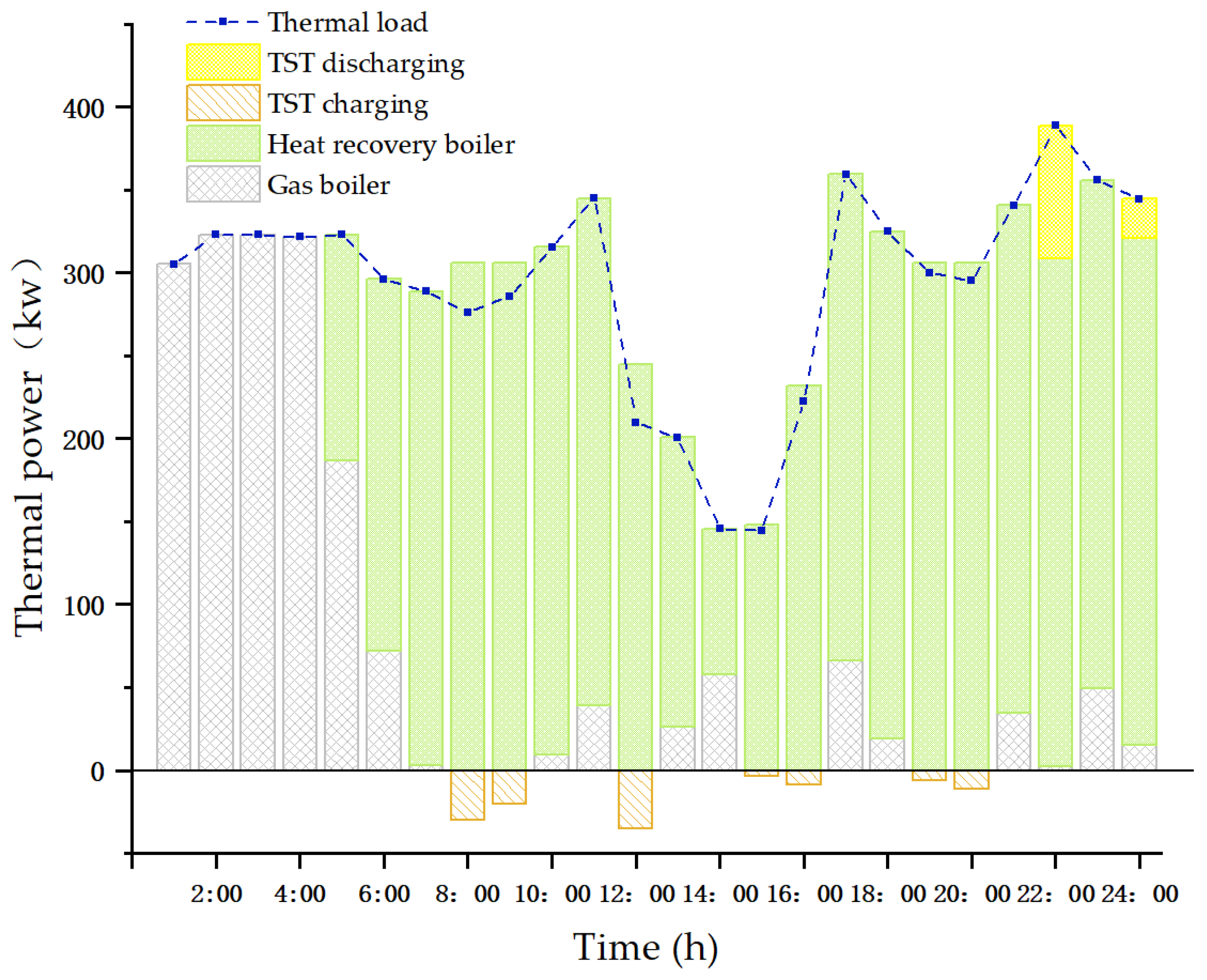
After the program calculation, Figure 8, Figure 9 and Figure 10 show the scheduling results of three different energy sources in the system at 24 hours a day. In addition, the dashed lines in the three figures represent the load prediction curves of the three energy sources respectively. In detail, as we can see in Figure 8, wind power and photovoltaic, as the base load, have priority in power generation and gas turbine, as the main system power supply unit, is in shutdown state between 0:00–4:00 PM because of its generating cost, which is higher than the power purchase cost from an external grid but is at peak load period basically at full output power since the electricity load is at its highest during the day. Furthermore, to achieve balance between supply and demand at the same time, the peak load period between 18:00 to 22:00 also curtails part of the electricity, called demand side management. It can be basically seen that part of the power supply beyond the power load prediction curve is consumed in the energy storage charging, electric chiller, and selling to the external power grid. Figure 9 illustrates the scheduling results of thermal energy. It can be observed that the thermal storage tank stores the excess heat energy in the time periods from 8:00 to 9:00, 12:00, 15:00 to 16:00, and 19:00 to 20:00 and releases thermal energy during 22:00 to 24:00, which realizes the decoupling of heat energy and electric energy and makes energy use more reasonable. This measure avoids energy loss and resource waste caused by excessive heat production by the gas turbine. Figure 10 describes the dispatching result with satisfaction of cooling load. It can be seen clearly from the image that the ice storage machine uses electricity to store ice in the off-peak load period (6:00–7:00) of electricity price, which can be observed is lower than the price at peak load (8:00–9:00) from Figure A2, and then releases cold energy at 8:00, so as to realize the division of the supply time of electric energy into cold energy, thus avoiding the high electricity price at peak load and saving the cost of electricity purchase.
5.3.3. Analysis of Purchasing and Selling Behavior
The results of electricity purchase and sale are also shown in Figure 8. To further analyze the behavior of electricity purchase and sale, the optimization results of electricity purchase and sale scheduling are plotted and analyzed separately.
The main driving factors of the power interaction between the IES and external grid can be divided into two categories: economic factors and operational demand factors. First of all, from the perspective of economic operation, such as between 0:00–7:00 period, IES adopts continuous external electricity purchasing strategy. Combined with the dispatching optimization results, it can be analyzed that the external power purchase price is lower than the marginal cost of the gas turbine’s power generation operation at this time. Consequently, the gas turbine chooses not to turn on, and the remaining electricity is purchased from the external grid to meet the load demand. However, the system sells part of the electricity to the external power grid during the periods from 8:00 to 12:00, 16:00-17:00, and 23:00 to 0:00. The reason is that the feed-in tariff, which is higher than the cost of generation, is at its highest during these periods. Therefore, after meeting the daily load, the rest of the electricity is still generated on grid. In this way, it is easy to earn profit through price differences, and economic efficiency of the system can be improved. Secondly, in the view of the system demand, when the generator capacity of the system is insufficient, in order to satisfy the power load demand of the system, it is necessary to purchase power from the external grid to fill the power gap, such as during the period from 18:00 to 20:00. It can be obviously observed from Figure A1 that the power load is in the maximum load period of the day. Due to the limitation of the maximum generating capacity, the system must purchase power from the external power grid to meet the power load demand gap, which is rigid demand.
5.3.4. Analysis of Battery Operation Results
The detail scheduling results of battery charge and discharge behavior are shown as follows:
As a whole, it can be seen from Figure 10 that there are two charging and discharging processes in the whole dispatching cycle. First of all, the first charge and discharge process is obviously an arbitrage behavior. During the period from 8:00 to 11:00, the load is in the peak load period and the electricity selling price reaches a maximum of 0.85 ¥/kwh. At this time, Figure 11 also shows the electricity selling behavior. According to Figure A1, the load is at a trough period between 0:00 and 7:00 and the purchase price is as low as 0.35 ¥/kwh, so it corresponds to the purchase behavior in Figure 12. From the perspective of price difference, it is easy to find that the per unit of electricity profit margin is 0.5 ¥. Therefore, energy storage will automatically use the charging and discharging mechanism to purchase electricity when the price is low and will sell this part of electric quantity when the price is highest. However, because of the restriction of maximum energy storage capacity, the maximum arbitrage space is only a 15-kwh capacity. Moreover, observing the second charge and discharge process combined with TOU price in Figure A2, we can see that, during the period of 19:00–20:00, transactions also have arbitrage space but because of the load in the peak load period (as shown in Figure A1) and in this period of time, according to the results of the scheduling system, the gas turbine has been in a state of maximum power. At this time, the energy storage must be used as a temporary emergency power discharge to meet the power load demand, so the electricity is unable to be used for arbitrage. Figure 11 only has the purchase behavior between 19:00 and 20:00, which also confirms the process.
5.3.5. Analysis of Economic, Environmental Benefits, and Energy Efficiency of the CTED Model
To better demonstrate the gain effect of CTED on the system, this paper operates under three initial settings, namely the traditional operation mode, TED operation mode, and CTED operation mode and solves the problem to obtain the total system cost and penalty cost of CO2 emission as shown in the Figure 13 below.
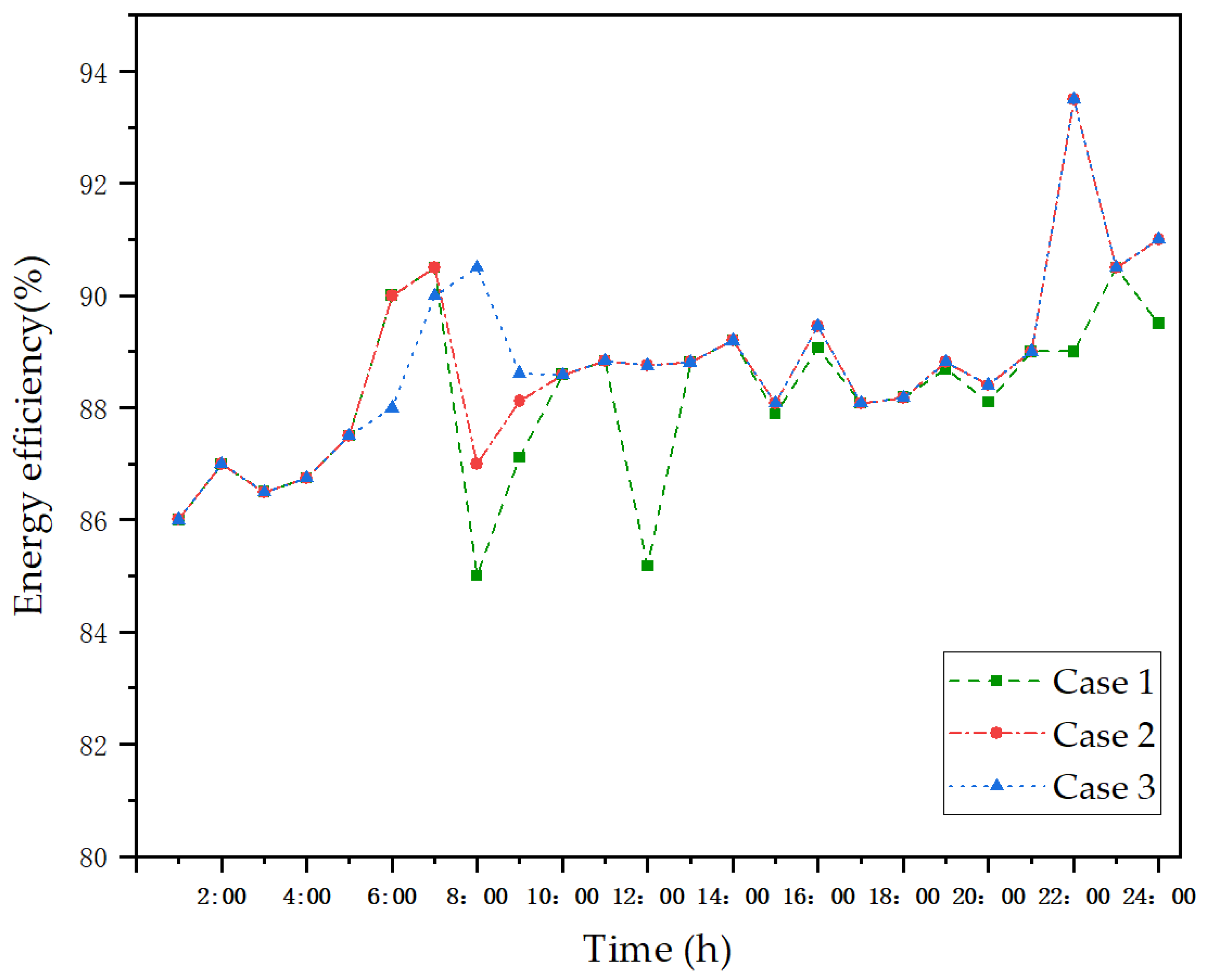
According to the data in the figure, the total cost and the penalty cost of CO2 emission of CTED operation mode (Case 3) are both the minimum values under the three modes. Combined with the analysis of operation results, IES can get rid of the traditional operation mode of “electricity is determined by heat” and “electricity is determined by cold” when heat storage and cooling storage equipment are added. To be specific, the extra heat generated by the gas turbine can be transferred and stored in the heat storage tank through pipelines. When the heat load rises, the heat energy can be released, avoiding the loss of heat energy and improving the use rate of energy. In the case of electric energy cooling energy, if the cooling storage equipment increases, it can realize the storage of cold at the trough of the load and the cooling at the peak load, which reasonably avoid the peak load electricity price period, save on the total cost of electricity purchase, and improve the flexibility and variability of energy supply. In conclusion, the CTED mode not only enhances the flexibility of energy supply but also reduces the operating cost of the system and the penalty cost of CO2 emission. That is to say, the flexible transformation of IES enhances the flexibility, economy, and environmental protection of the system operation. Figure 14 analyzes the energy efficiency of the system, and the calculation results are as follows.
The three curves in Figure 14 represent the change trend of energy efficiency at 24 h under three different cases. Obviously, Case 2 and Case 3 show the same energy efficiency most of the time, and the difference is only reflected in the 5:00–9:00 interval. Combined with the image above, it can be concluded that the operation mechanism of the cold storage equipment leads to this phenomenon. The ice storage device stores the cold between 5:00 and 7:00, which converts a piece of electrical energy into cold energy, and it is stored in the cold storage system, reducing the energy efficiency. During the period from 7:00 to 9:00, the cooling storage device releases cold, which reduces the intake of electric energy and improves energy efficiency. However, the energy efficiency curve of Case 1 (green line) is lower than that of Case 2 and Case 3 at many time periods. As is known, the gas turbine generates heat while generating electricity, but in order to meet the electrical load demand of the system, the gas turbine generates surplus heat synchronously. It is precisely because of the lack of heat storage in Case 1 that this part of heat is lost. In Case 2 and Case 3, the excess heat of gas turbine is stored centrally, which reduces the loss of heat energy. At the same time, the heat energy is released during the peak period of thermal load, realizing the efficient use of energy and avoiding the waste of resources.
5.3.6. Sensitivity Analysis
• λ factor sensitivity analysis
Although the uncertainty of photovoltaic and wind power output is described by scene classification, the expected operating cost is still only an expected value that may occur, but there are still some risks. This paper uses CVaR risk control theory to reasonably avoid the economic risk of operating cost deviation. Since the subjective propensity coefficient λ in Equation (2) is externally set according to the degree of risk appetite, the value of λ will ultimately affect the decision-making result of the system. Therefore, Figure 14 shows the pareto boundary curve formed by the total expected cost with its CVaR under different λ.
According to the graph, the expected total cost of IES increases with λ but the CVaR of its actual cost decreases. The reason is that the larger λ in this model is, the more risk-neutral scheduling strategies IES will be adopted for random fluctuations of wind power and photovoltaic output. At this moment, the scheduling strategy can better reflect the pursuit of the scheduling target with the minimum expected total cost, but it cannot resist the interference of renewable energy output uncertainty on the whole system. On the contrary, the smaller λ is, the more IES tends to pursue risk-averse scheduling strategy in the scheduling process and the more IES operators will adopt a conservative scheduling strategy. Therefore, as clearly observed from Figure 15, IES operators cannot pursue the improvement of the other targets without compromising either target. The relation curve shown in Figure 15 is a pareto frontier curve (with respect to coefficient λ). In practical decision-making, IES operators’ choice of λ cannot be based on this curve. The specific value of λ should be determined by the ultimate decision-maker’s subjective preference for risk.
• Sensitivity analysis of carbon emission penalty coefficient
In this numerical example, the penalty coefficient of CO2 emission is given artificially. In order to study the impact of the penalty price coefficient on carbon emission of IES, this paper sets the coefficient as 0.1, 0.3, 0.5, 0.7, 1.0, and 1.5 and substitutes them into the model to solve them separately. The relationship curve between the penalty price coefficient and CO2 emission is illustrated in Figure 16. The graph demonstrates that, along with the strengthening of penalties to the CO2 emissions, CO2 emissions reduced gradually but the downward trend gradually slows down. CO2 emissions in this system are only related to the consumption of natural gas and the purchase of electricity from external power grid. It can be boldly assumed that, when the consumption of natural gas and the external purchase of electricity reach the limit of functional constraints, CO2 emissions will not decline anymore because the functional requirements of the system must be met.
6. Conclusions
First of all, this paper makes an in-depth summary of the development of the operation mode of the current IES, analyzes the disadvantages of the operation of the traditional energy system, and puts forward a new operation mode of flexible transformation, which constructs a FIES architecture with heat and cold storage technology. At the same time, the scheduling model of FIES with low carbon economy is established with the optimal scheduling target of system operating economy and minimum expected cost of carbon dioxide emission. Stochastic optimization and FCM-CCQ clustering method are used to describe typical output scenarios of wind and solar power. In terms of system risk control, the risk control theory based on CVaR is proposed and the reasonable control module of system risk is introduced into the objective function to further improve the established model. Finally, comparing with previous studies, the following differences are drawn through the analysis of simulation examples in this paper:
- Apart from the operation mode of IES in other research, the IES after transformation is in good operation condition as a whole, and the cold, hot, and electric loads are satisfied, which ensures the reliability of the energy supply of the system. At the same time, heat storage, electricity storage, and cold storage equipment are charged/discharged at appropriate times, which further improves the flexibility of the overall operation of the system and reflects the principles of economical, reliable, and safe operation of IES.
- Meanwhile, the system is optimized from the perspective of carbon emission and the environmental benefit of system operation can be improved after flexible transformation. Based on the analysis of carbon emission penalty price mechanism, the conclusion is that CO2 emission will decrease with the increase of penalty price coefficient but, when it reaches the critical value, it cannot be further reduced due to the constraint of energy supply demand.
- In terms of energy-use efficiency of the system, compared with the original IES in other research, the flexible comprehensive energy system can integrally improve the energy-use efficiency and strengthen the rationality of the use of limited resources.
- Compared with the traditional clustering method, the FCM-CCQ algorithm presented in this paper can better explain the number selection of clustering centers and the clustering analysis process is more scientific and logical.
- The stochastic optimization method considering CVaR is adopted to fully consider the risk existing in the system operation process, which previous studies did not take account into. Risk management selects the corresponding weighting factor λ according to the decision maker’s different degrees of risk preference, so the corresponding scheduling optimization strategy is adopted pertinently.
Finally, the FIES proposed in this paper only makes some basic researches at the level of dispatching and control, providing references for decision makers to realize control of the global dispatching strategy of the system. However, the operational constraints of power grid and natural gas network need to be considered more in the operation of the actual integrated energy system. Thus, future research can also consider the flexibility of network transformation, so as to form a flexible regional integrated energy system.
Author Contributions
H.L. supervised the proposed research work, conceptualized the proposed research work, programmed and analyzed the methodology, and wrote the original draft. S.N. helped in collecting the data, reviewing the writing and editing with validation of the research work.
Funding
This research was funded by 2020 Key Scientific Research Projects of Henan Higher Institutions (20A6300352018), 2018 Key Scientific and Technological Project of Henan Province (182102210442) and 2019 Youth Scholar Supporting Program of Henan Province (2019-179).
Conflicts of Interest
The authors declare no conflict of interest.
Appendix A
Figure A1.
Curve of cold, thermal, and electric load.

Figure A2.
Time-of-Use (TOU) price curve for purchasing and selling electricity.


Table A1.
IES basic component physical data.
| System Element | Pmin(kw) | Pmax(kw) | Ramp Rate (kw/h) | Maintenance Cost (¥/kwh) | Energy Conversion Efficiency |
|---|---|---|---|---|---|
| Gas turbine | 30 | 200 | 60 | 0.1685 | 0.8 |
| Heat exchanger | 0 | 600 | — | 0.08 | 0.85 |
| Gas boiler | 0 | 500 | — | 0.02 | 0.73 |
| Wind power | 0 | 150 | — | 0.11 | 0.95 |
| Photovoltaic power | 0 | 120 | — | 0.08 | 0.95 |
| Electric chiller | 0 | 13 | — | 0.03 | 4 |
| Heating coil | 0 | 10 | — | 0.06 | 0.88 |
Table A2.
Physical data of energy storage device.
| Energy Storing Device | Initial Energy Storage (kwh) | Rated Energy Capacity (kwh) | Discharge/Charge Efficiency | PCmax (kw) | PDmax (kw) | Self-Discharge Rate | Maintenance Cost (¥/kwh) |
|---|---|---|---|---|---|---|---|
| Battery | 5 | 20 | 0.95 | 5 | 10 | 0.05 | 0.02 |
| Thermal storage tank | 16 | 160 | 0.95 | 80 | 80 | 0.0.5 | 0.015 |
| Cooling storage tank | 10 | 100 | 0.95 | 80 | 80 | 0.0.5 | 0.015 |
References
- Simionescu, M.; Bilan, Y.; Gędek, S.; Streimikiene, D. The Effects of Greenhouse Gas Emissions on Cereal Production in the European Union. Sustainability 2019, 11, 3433. [Google Scholar] [CrossRef]
- Hnatyshyn, M. Decomposition analysis of the impact of economic growth on ammonia and nitrogen oxides emissions in the European Union. J. Int. Stud. 2018, 11, 201–209. [Google Scholar] [CrossRef] [Green Version]
- Kharlamova, G.; Nate, S.; Chernyak, O. Renewable energy and security for Ukraine: Challenge or smart way. J. Int. Stud. 2016, 9, 88–115. [Google Scholar] [CrossRef] [PubMed]
- Kasperowicz, R.; Pinczyński, M.; Khabdullin, A. Modeling the power of renewable energy sources in the context of classical electricity system transformation. Int. Stud. 2017, 10, 264–272. [Google Scholar] [CrossRef]
- Shindina, T.; Streimikis, J.; Sukhareva, Y.; Nawrot, Ł. Social and Economic Properties of the Energy Markets. Econ. Sociol. 2018, 11, 334–344. [Google Scholar] [CrossRef]
- Lv, C.; Yu, H.; Li, P.; Wang, C.; Xu, X.; Li, S.; Wu, J. Model predictive control based robust scheduling of community integrated energy system with operational flexibility. Appl. Energy 2019, 243, 250–265. [Google Scholar] [CrossRef]
- Safari, F.; Dincer, I. Assessment and optimization of an integrated wind power system for hydrogen and methane production. Energy Convers. Manag. 2018, 177, 693–703. [Google Scholar] [CrossRef]
- Yang, Z.; Gao, C.; Zhao, M. Coordination of integrated natural gas and electrical systems in day-ahead scheduling considering a novel flexible energy-use mechanism. Energy Convers. Manag. 2019, 196, 117–126. [Google Scholar] [CrossRef]
- Blázquez, C.S.; Borge-Diez, D.; Nieto, I.M.; Martín, A.F.; González-Aguilera, D. Technical optimization of the energy supply in geothermal heat pumps. Geothermics 2019, 81, 133–142. [Google Scholar] [CrossRef]
- Suresh, N.; Thirumalai, N.; Dasappa, S. Modeling and analysis of solar thermal and biomass hybrid power plants. Appl. Therm. Eng. 2019, 160, 114121. [Google Scholar] [CrossRef]
- Subramanian, V.; Das, T.K.; Kwon, C.; Gosavi, A. A data-driven methodology for dynamic pricing and demand response in electric power networks. Electr. Power Syst. Res. 2019, 174, 105869. [Google Scholar] [CrossRef]
- Parra, D.; Norman, S.A.; Walker, G.S.; Gillott, M. Optimum community energy storage for renewable energy and demand load management. Appl. Energy 2017, 200, 358–369. [Google Scholar] [CrossRef]
- Yang, Y.; Wu, K.; Long, H.; Gao, J.; Yan, X.; Kato, T.; Suzuoki, Y. Integrated electricity and heating demand-side management for wind power integration in China. Energy 2014, 78, 235–246. [Google Scholar] [CrossRef]
- Tvaronavičienė, M.; Prakapienė, D.; Garškaitė-Milvydienė, K.; Prakapas, R.; Nawrot, Ł. Energy efficiency in the long run in the selected European countries. Econ. Sociol. 2018, 11, 245–254. [Google Scholar] [CrossRef]
- Bazmohammadi, N.; Tahsiri, A.; Anvari-Moghaddam, A.; Guerrero, J.M. A hierarchical energy management strategy for interconnected microgrids considering uncertainty. Int. J. Electr. Power Energy Syst. 2019, 109, 597–608. [Google Scholar] [CrossRef]
- Shen, X.; Guo, Q.; Xu, Y.; Sun, H. Robust planning of regional integrated energy system considering multi-energy load uncertainty. Power Syst. Autom. 2019, 43, 34–45. [Google Scholar]
- Nikoobakht, A.; Aghaei, J.; Fallahzadeh-Abarghouei, H.; Hemmati, R. Flexible Co-Scheduling of Integrated Electrical and Gas Energy Networks under Continuous and Discrete Uncertainties. Energy 2019, 182, 201–210. [Google Scholar] [CrossRef]
- Marino, C.; Marufuzzaman, M.; Hu, M.; Sarder, M. Developing a CCHP-microgrid operation decision model under uncertainty. Comput. Ind. Eng. 2018, 115, 354–367. [Google Scholar] [CrossRef]
- Shams, M.H.; Shahabi, M.; Kia, M.; Heidari, A.; Lotfi, M.; Shafie-khah, M.; Catalão, J.P.S. Optimal operation of electrical and thermal resources in microgrids with energy hubs considering uncertainties. Energy 2019, 187, 115949. [Google Scholar] [CrossRef]
- Hemmati, M.; Mohammadi-Ivatloo, B.; Ghasemzadeh, S.; Reihani, E. Risk-based optimal scheduling of reconfigurable smart renewable energy based microgrids. Int. J. Electr. Power Energy Syst. 2018, 101, 415–428. [Google Scholar] [CrossRef]
- Abdollahi, G.; Meratizaman, M. Multi-objective approach in thermoenvironomic optimization of a small-scale distributed CCHP system with risk analysis. Energy Build. 2011, 43, 3144–3153. [Google Scholar] [CrossRef]
- Zhang, T.; Wang, M.; Wang, P.; Gu, J.; Zheng, W.; Dong, Y. Bi-stage stochastic model for optimal capacity and electric cooling ratio of CCHPs—A case study for a hotel. Energy Build. 2019, 194, 113–122. [Google Scholar] [CrossRef]
- Zhu, J.; Jiang, Z.; Evangelidis, G.D.; Zhang, C.; Pang, S.; Li, Z. Efficient registration of multi-view point sets by K-means clustering. Inf. Sci. 2019, 488, 205–218. [Google Scholar] [CrossRef] [Green Version]
- Fadaei, A.H.; Khasteh, S.H. Enhanced K-means re-clustering over dynamic networks. Expert Syst. Appl. 2019, 132, 126–140. [Google Scholar] [CrossRef]
- Jin, R.; Weng, G. A robust active contour model driven by fuzzy c-means energy for fast image segmentation. Digit. Signal Process. 2019, 90, 100–109. [Google Scholar] [CrossRef]
- Deng, Z.H.; Qiao, H.H.; Song, Q.; Gao, L. A complex network community detection algorithm based on label propagation and fuzzy C-means. Phys. A Stat. Mech. Appl. 2019, 519, 217–226. [Google Scholar] [CrossRef]
- Wu, X.; Wu, B.; Sun, J.; Qiu, S.; Li, X. A hybrid fuzzy K-harmonic means clustering algorithm. Appl. Math. Model. 2015, 39, 3398–3409. [Google Scholar] [CrossRef]
- Hung, C.H.; Chiou, H.M.; Yang, W.N. Candidate groups search for K-harmonic means data clustering. Appl. Math. Model. 2013, 37, 10123–10128. [Google Scholar] [CrossRef]
- Yang, J.; Ning, C.; Deb, C.; Zhang, F.; Cheong, D.; Lee, S.E.; Sekhar, C.; Tham, K.W. k-Shape clustering algorithm for building energy usage patterns analysis and forecasting model accuracy improvement. Energy Build. 2017, 146, 27–37. [Google Scholar] [CrossRef]
- Morales, J.M.; Conejo, A.J.; Madsen, H.; Pinson, P.; Zugno, M. Integrating Renewables in Electricity Markets: Operational Problems; Springer Science & Business Media: New York, NY, USA, 2013; pp. 142–158. [Google Scholar]
- Ding, H.; Pinson, P.; Hu, Z.; Song, Y. Optimal offering and operating strategies for wind-storage systems with linear decision rules. IEEE Trans. Power Syst. 2016, 31, 4755–4764. [Google Scholar] [CrossRef]
- Liu, Z.; Chen, Y.; Zhuo, R.; Jia, H. Energy storage capacity optimization for autonomy microgrid considering CHP and EV scheduling. Appl. Energy 2018, 210, 1113–1125. [Google Scholar] [CrossRef]
- Wang, H.; Yin, W.; Abdollahi, E.; Lahdelma, R.; Jiao, W. Modelling and optimization of CHP based district heating system with renewable energy production and energy storage. Appl. Energy 2015, 159, 401–421. [Google Scholar] [CrossRef]
- Wang, D.; Qiu, J.; Reedman, L.; Meng, K.; Lai, L.L. Two-stage energy management for networked microgrids with high renewable penetration. Appl. Energy 2018, 226, 39–48. [Google Scholar] [CrossRef]
- Zhou, X.; Ai, Q. Distributed economic and environmental dispatch in two kinds of CCHP microgrid clusters. Int. J. Electr. Power Energy Syst. 2019, 112, 109–126. [Google Scholar] [CrossRef]
- Gu, W.; Tang, Y.; Peng, S.; Wang, D.; Sheng, W.; Liu, K. Optimal configuration and analysis of combined cooling, heating, and power microgrid with thermal storage tank under uncertainty. J. Renew. Sustain. Energy 2015, 7, 013104. [Google Scholar] [CrossRef]
- Luo, F.; Yang, J.; Dong, Z.Y.; Meng, K.; Wong, K.P.; Qiu, J. Short-term operational planning framework for virtual power plants with high renewable penetrations. IET Renew. Power Gener. 2016, 10, 623–633. [Google Scholar] [CrossRef]
- Wang, Z.; Shi, Y.; Tang, Y.; Men, X.; Cao, J.; Wang, H. Low carbon economy operation and energy efficiency analysis of integrated energy system considering LCA energy chain and carbon trading mechanism. Chin. J. Electr. Eng. 2019, 39, 1614–1626. [Google Scholar]
- Ban, O.I.; Ban, A.I.; Tuşe, D.A. Importance–performance analysis by fuzzy C-means algorithm. Expert Syst. Appl. 2016, 50, 9–16. [Google Scholar] [CrossRef]
- Dong, J.; Yang, P.; Nie, S. Day-Ahead Scheduling Model of the Distributed Small Hydro-Wind-Energy Storage Power System Based on Two-Stage Stochastic Robust Optimization. Sustainability 2019, 11, 2829. [Google Scholar] [CrossRef]
- Xu, H.; Jiao, Y.; Pu, L.; He, N.; Wang, Y.; Tan, Z. Stochastic scheduling optimization model of wind-wind combustion storage virtual power plant considering uncertainty and demand response. Power Grid Technol. 2017, 41, 3590–3597. [Google Scholar]
- Zhou, B.; Lv, L.; Gao, H.; Liu, J.; Chen, Q.; Tan, X. Research on robust trading strategies for multi-virtual power plants. Power Grid Technol. 2008, 42, 2694–2703. [Google Scholar]
- Li, R.; Hu, Z.; Duan, X. Monthly transaction model and daily operation optimization strategy for agents of electric bus charging station. Power Constr. 2019, 40, 27–34. [Google Scholar]
- Luo, Z.; Wu, Z.; Li, Z.; Cai, H.; Li, B.; Gu, W. A two-stage optimization and control for CCHP microgrid energy management. Appl. Therm. Eng. 2017, 125, 513–522. [Google Scholar] [CrossRef]
Figure 1.
The structure of flexible integrated energy systems (FIES).

Figure 2.
The piecewise linearized curve between thermal power and electrical power.

Figure 3.
The solution flow chart of fuzzy c-mean-clustering comprehensive quality (FCM-CCQ).

Figure 4.
The solution flow chart of stochastic optimization model considering conditional value at risk (CVaR).
Figure 4.
The solution flow chart of stochastic optimization model considering conditional value at risk (CVaR).

Figure 5.
Three operating mode structure comparison: (a) Traditional operation mode; (b) thermoelectric decoupling (TED) operation mode; and (c) cooling, thermal, and electricity decoupling (CTED) operation mode.
Figure 5.
Three operating mode structure comparison: (a) Traditional operation mode; (b) thermoelectric decoupling (TED) operation mode; and (c) cooling, thermal, and electricity decoupling (CTED) operation mode.

Figure 6.
The marginal benefit curve of clustering.

Figure 7.
Ten typical output scenarios of wind and photovoltaic units.

Figure 8.
Power supply scheduling results.

Figure 9.
Thermal energy supply scheduling results.

Figure 10.
Cold energy supply scheduling results.

Figure 11.
Interaction results with external grid.

Figure 12.
Battery charge and discharge results.

Figure 13.
Cost comparison of three cases.

Figure 14.
Comparison of energy efficiency in three cases.

Figure 15.
The pareto frontier curve for total cost and CVaR.

Figure 16.
Relation curve between CO2 emission and penalty price coefficient.

© 2019 by the authors. Licensee MDPI, Basel, Switzerland. This article is an open access article distributed under the terms and conditions of the Creative Commons Attribution (CC BY) license (http://creativecommons.org/licenses/by/4.0/).
Share and Cite
MDPI and ACS Style
Liu, H.; Nie, S. Low Carbon Scheduling Optimization of Flexible Integrated Energy System Considering CVaR and Energy Efficiency. Sustainability 2019, 11, 5375. https://doi.org/10.3390/su11195375
AMA Style
Liu H, Nie S. Low Carbon Scheduling Optimization of Flexible Integrated Energy System Considering CVaR and Energy Efficiency. Sustainability. 2019; 11(19):5375. https://doi.org/10.3390/su11195375
Chicago/Turabian StyleLiu, Hang, and Shilin Nie. 2019. "Low Carbon Scheduling Optimization of Flexible Integrated Energy System Considering CVaR and Energy Efficiency" Sustainability 11, no. 19: 5375. https://doi.org/10.3390/su11195375
Note that from the first issue of 2016, this journal uses article numbers instead of page numbers. See further details here.