
Urban Land Extraction Using VIIRS Nighttime Light Data: An Evaluation of Three Popular Methods


Abstract
:
1. Introduction
2. Study Area and Data
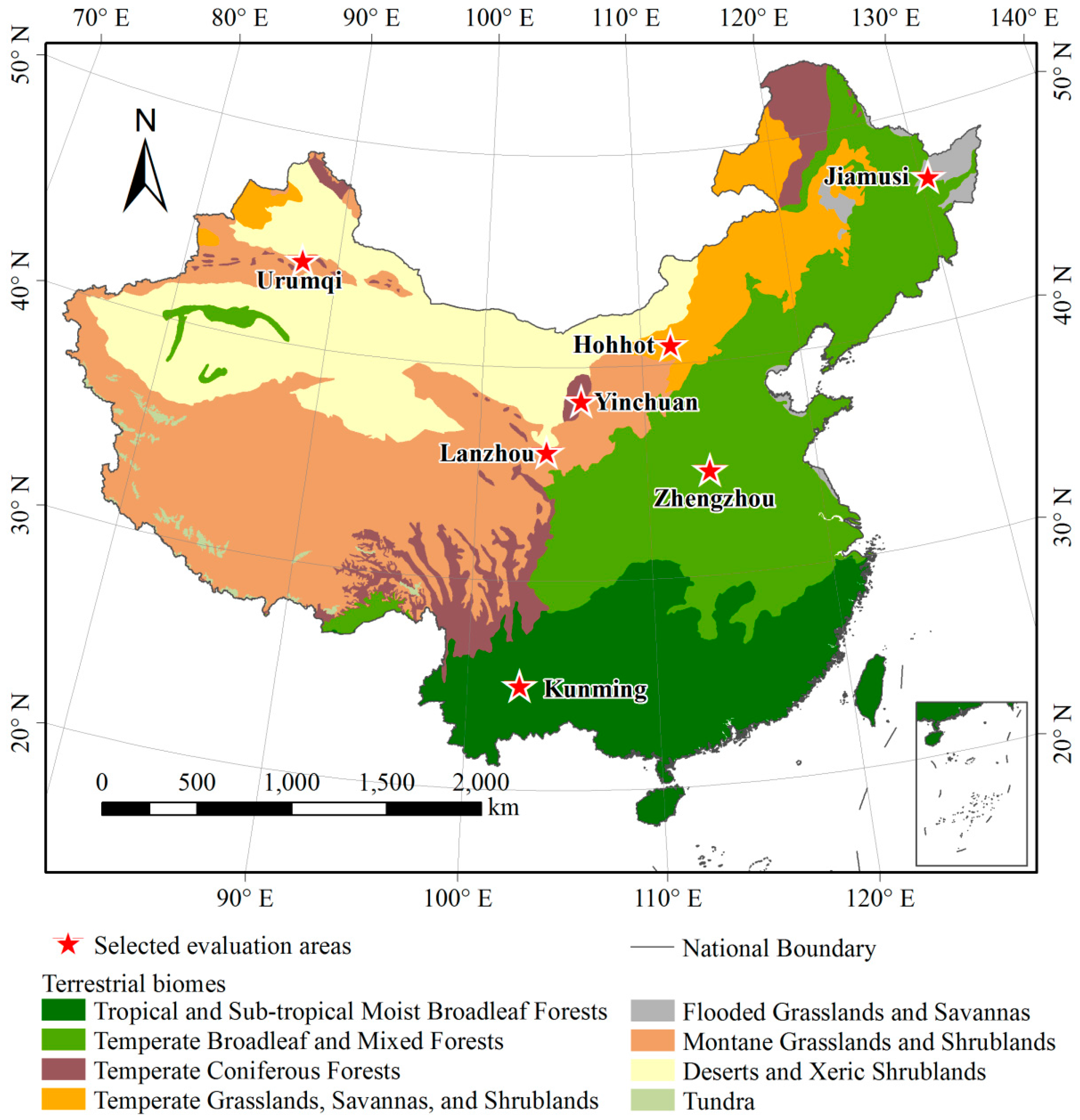
2.1. Study Area
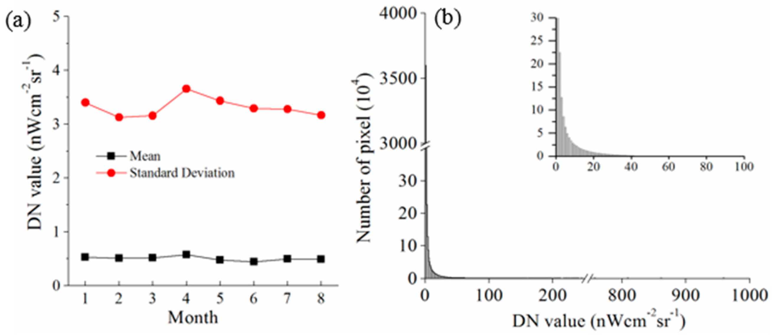
2.2. Data
3. Method
3.1. Extraction of Urban Land Area based on Different Methods
3.1.1. Local-Optimized Thresholding (LOT)
3.1.2. Vegetation-Adjusted Nighttime Light Urban Index (VANUI)
3.1.3. Integrated Nighttime Lights, Normalized Difference Vegetation Index, and Land Surface Temperature Support Vector Machine Classification (INNL-SVM)
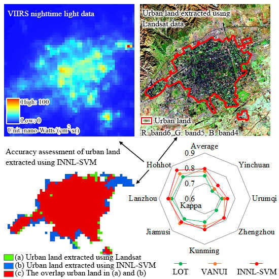
3.2. Accuracy Assessment of Urban Land
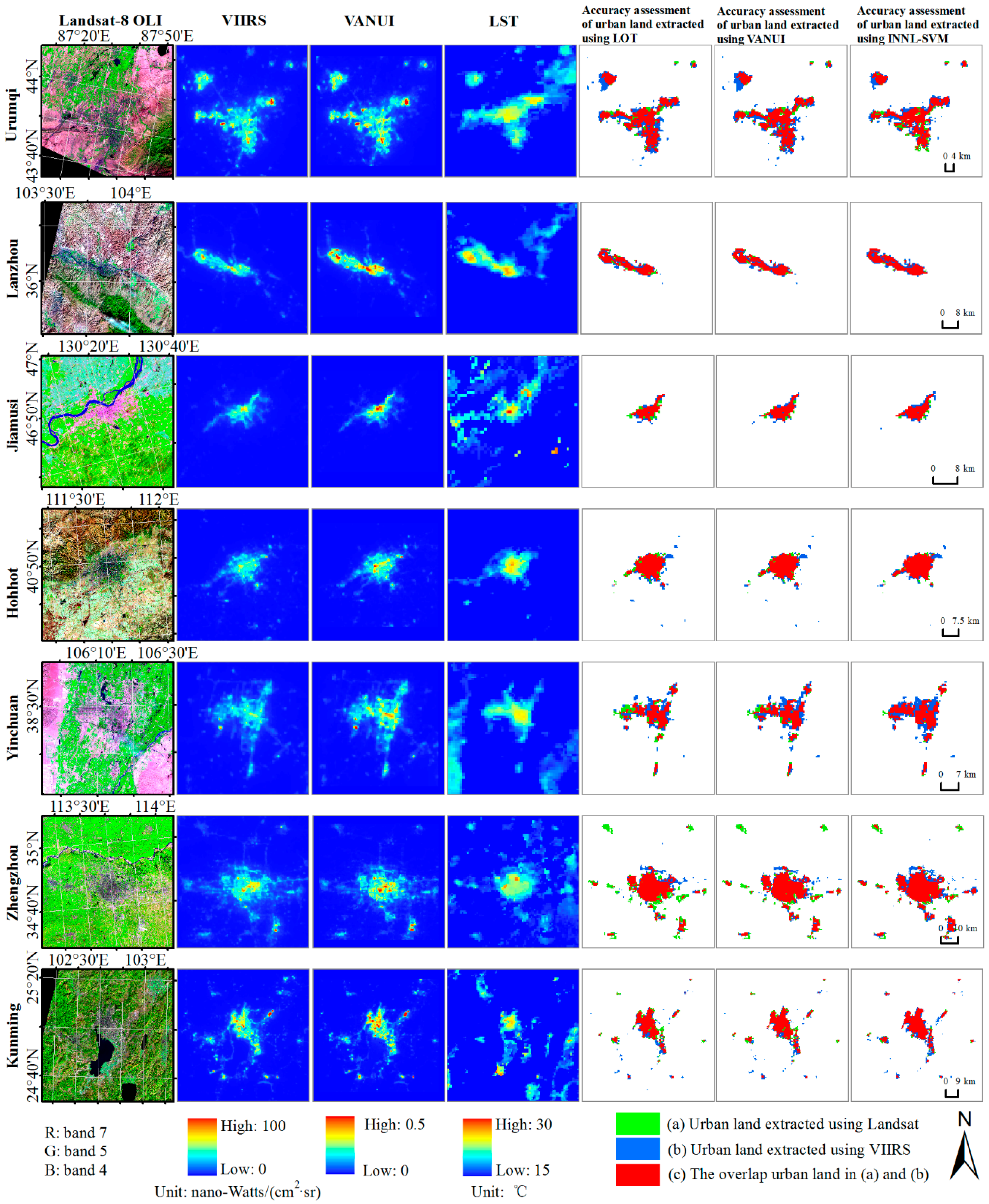
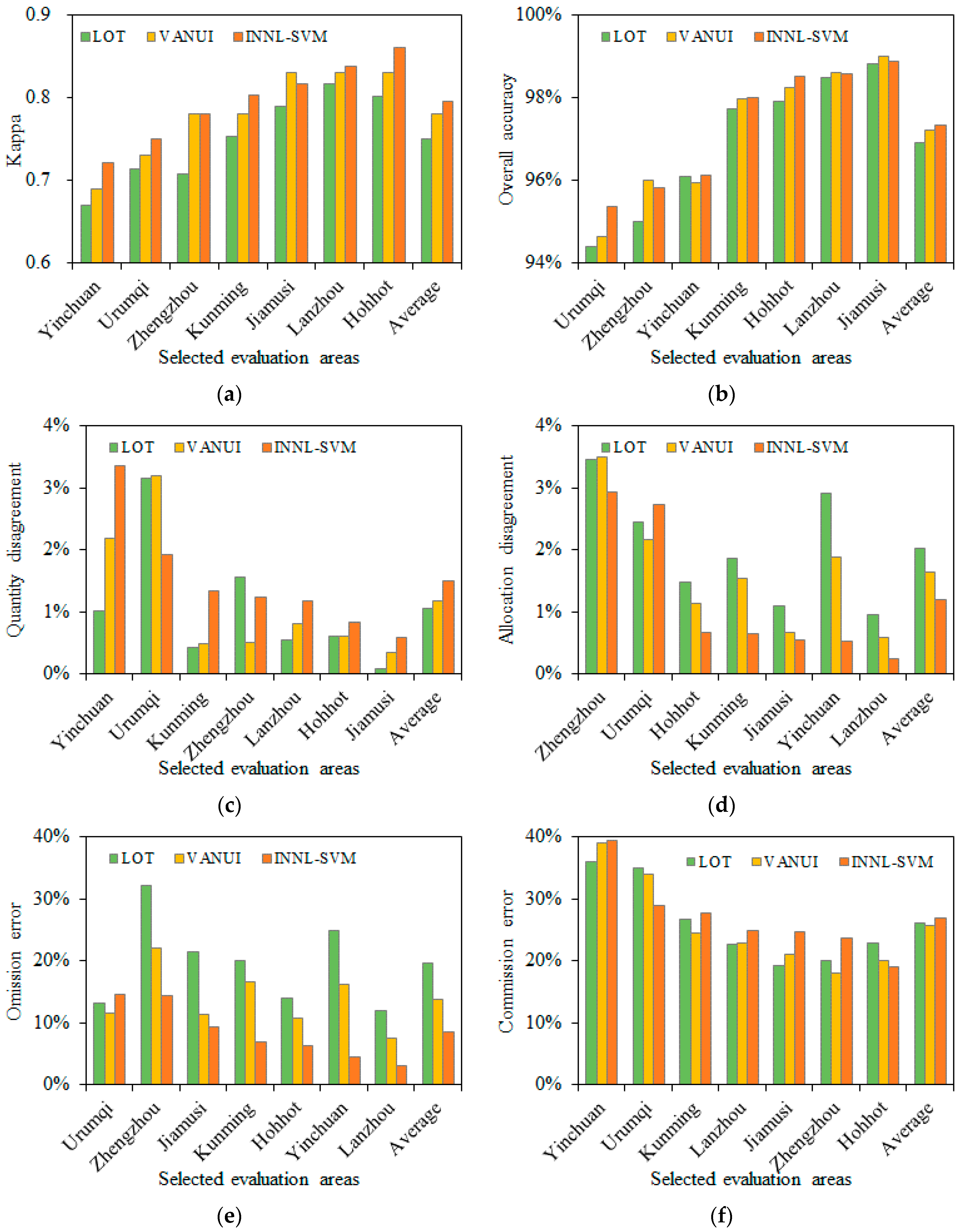
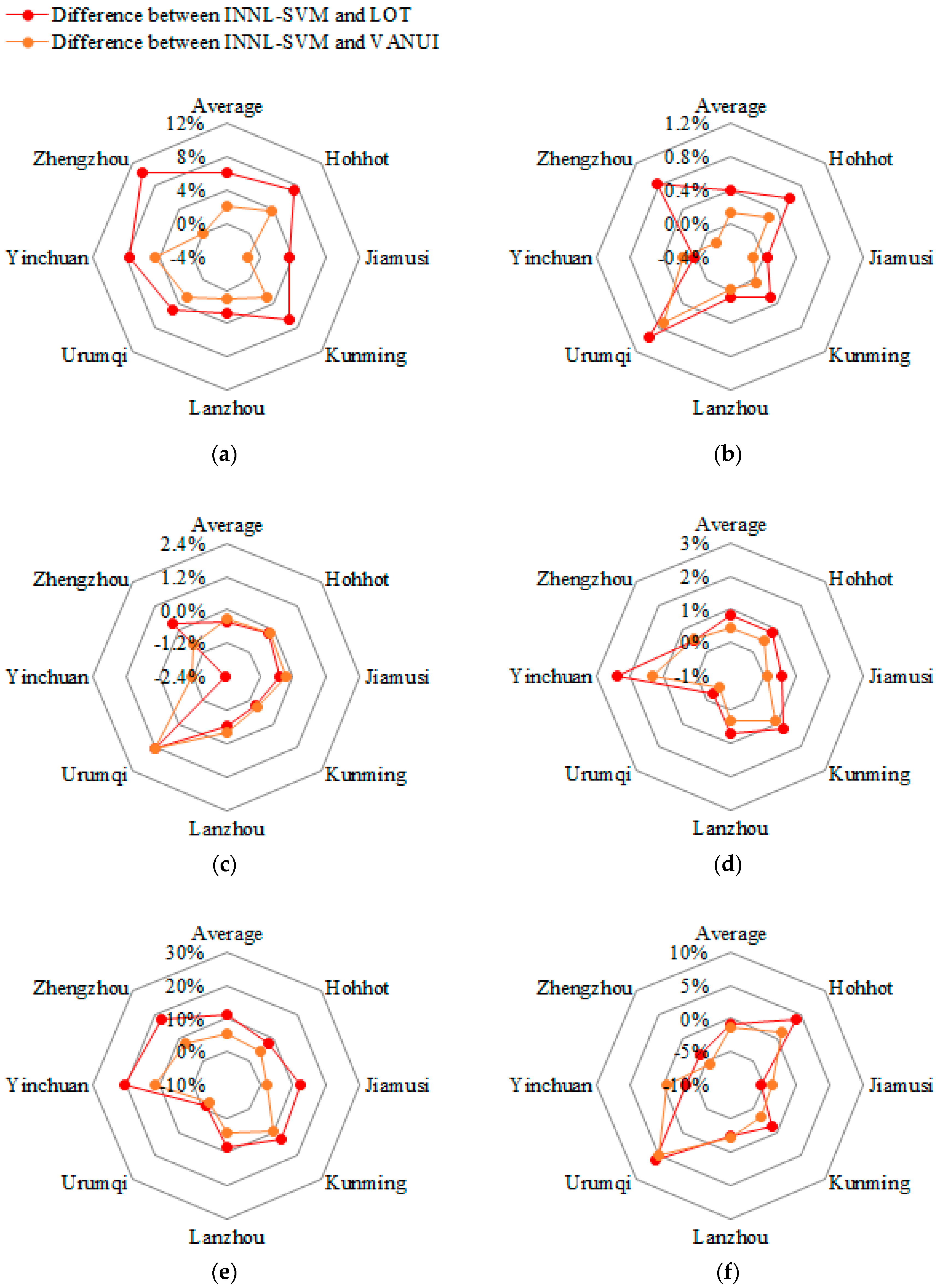
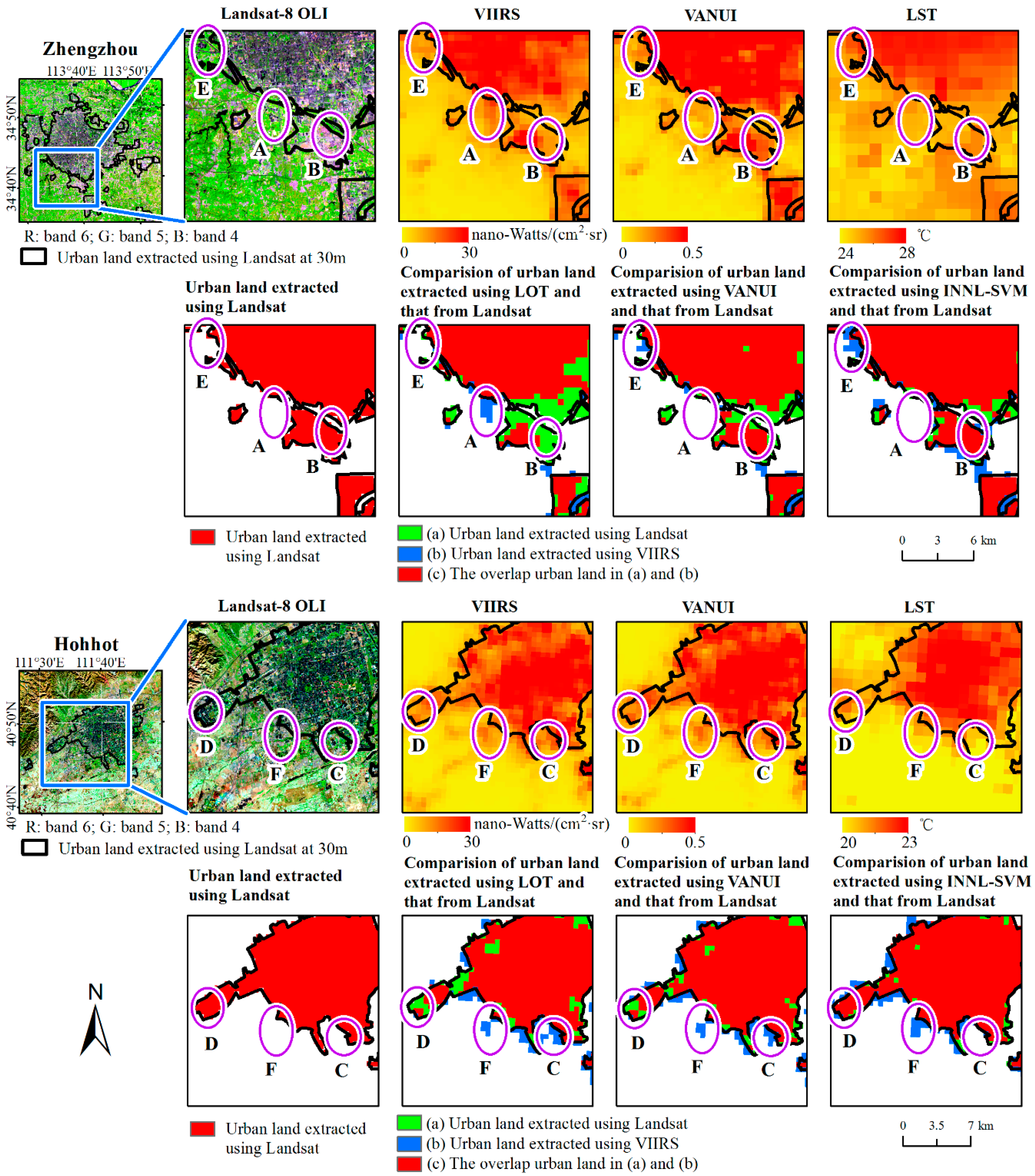
4. Results
5. Discussion
5.1. INNL-SVM Provides a Reliable Approach for Rapidly and Accurately Extracting Urban Land Area Using VIIRS Nighttime Light Data
6. Conclusions
Acknowledgments
Author Contributions
Conflicts of Interest
References
- Grimm, N.B.; Faeth, S.H.; Golubiewski, N.E.; Redman, C.L.; Wu, J.G.; Bai, X.M.; Briggs, J.M. Global change and the ecology of cities. Science 2008, 319, 756–760. [Google Scholar] [CrossRef] [PubMed]
- Seto, K.C.; Fragkias, M.; Guneralp, B.; Reilly, M.K. A meta-analysis of global urban land expansion. PLoS ONE 2011, 6, e23777. [Google Scholar] [CrossRef] [PubMed]
- Wu, J. Urban ecology and sustainability: The state-of-the-science and future directions. Landsc. Urban Plan. 2014, 125, 209–221. [Google Scholar] [CrossRef]
- Angel, S.; Parent, J.; Civco, D.L.; Blei, A.; Potere, D. The dimensions of global urban expansion: Estimates and projections for all countries, 2000–2050. Prog. Plan. 2011, 75, 53–107. [Google Scholar] [CrossRef]
- He, C.; Liu, Z.; Tian, J.; Ma, Q. Urban expansion dynamics and natural habitat loss in China: A multiscale landscape perspective. Glob. Chang. Biol. 2014, 20, 2886–2902. [Google Scholar] [CrossRef] [PubMed]
- Liu, Z.; He, C.; Wu, J. General spatiotemporal patterns of urbanization: An examination of 16 world cities. Sustainability 2016, 8, 41. [Google Scholar] [CrossRef]
- Liu, Z.; He, C.; Wu, J. The relationship between habitat loss and fragmentation during urbanization: An empirical evaluation from 16 world cities. PLoS ONE 2016, 11, e0154613. [Google Scholar] [CrossRef] [PubMed]
- Xu, M.; He, C.; Liu, Z.; Dou, Y. How did urban land expand in China between 1992 and 2015? A multi-scale landscape analysis. PLoS ONE 2016, 11, e0154839. [Google Scholar] [CrossRef] [PubMed]
- Seto, K.C.; Guneralp, B.; Hutyra, L.R. Global forecasts of urban expansion to 2030 and direct impacts on biodiversity and carbon pools. Proc. Natl. Acad. Sci. USA 2012, 109, 16083–16088. [Google Scholar] [CrossRef] [PubMed]
- Liu, Z.; He, C.; Zhou, Y.; Wu, J. How much of the world’s land has been urbanized, really? A hierarchical framework for avoiding confusion. Landsc. Ecol. 2014, 29, 763–771. [Google Scholar] [CrossRef]
- Shi, K.; Huang, C.; Yu, B.; Yin, B.; Huang, Y.; Wu, J. Evaluation of NPP-VIIRS night-time light composite data for extracting built-up urban areas. Remote Sens. Lett. 2014, 5, 358–366. [Google Scholar] [CrossRef]
- Shi, K.; Yu, B.; Huang, Y.; Hu, Y.; Yin, B.; Chen, Z.; Chen, L.; Wu, J. Evaluating the ability of NPP-VIIRS nighttime light data to estimate the gross domestic product and the electric power consumption of China at multiple scales: A comparison with DMSP-OLS data. Remote Sens. 2014, 6, 1705–1724. [Google Scholar] [CrossRef]
- Liao, L.B.; Weiss, S.; Mills, S.; Hauss, B. Suomi NPP VIIRS day-night band on-orbit performance. J. Geophys. Res. Atmos. 2013, 118, 12705–12718. [Google Scholar] [CrossRef]
- Chen, J.; Chen, J.; Liao, A.; Cao, X.; Chen, L.; Chen, X.; He, C.; Han, G.; Peng, S.; Lu, M.; et al. Global land cover mapping at 30 m resolution: A pok-based operational approach. ISPRS J. Photogramm. Remote Sens. 2015, 103, 7–27. [Google Scholar] [CrossRef]
- Shi, K.F.; Yu, B.L.; Hu, Y.J.; Huang, C.; Chen, Y.; Huang, Y.X.; Chen, Z.Q.; Wu, J.P. Modeling and mapping total freight traffic in China using NPP-VIIRS nighttime light composite data. GISci. Remote Sens. 2015, 52, 274–289. [Google Scholar] [CrossRef]
- Yu, B.; Shi, K.; Hu, Y.; Huang, C.; Chen, Z.; Wu, J. Poverty evaluation using NPP-VIIRS nighttime light composite data at the county level in China. IEEE J. Sel. Top. Appl. Earth Obs. Remote Sens. 2015, 8, 1217–1229. [Google Scholar] [CrossRef]
- Elvidge, C.D.; Baugh, K.E.; Zhizhin, M.; Hsu, F.-C. Why VIIRS data are superior to DMSP for mapping nighttime lights. Proc. Asia-Pac. Adv. Netw. 2013, 35, 62–69. [Google Scholar] [CrossRef]
- Schueler, C.F.; Lee, T.F.; Miller, S.D. VIIRS constant spatial-resolution advantages. Int. J. Remote Sens. 2013, 34, 5761–5777. [Google Scholar] [CrossRef]
- Sharma, R.C.; Tateishi, R.; Hara, K.; Gharechelou, S.; Iizuka, K. Global mapping of urban built-up areas of year 2014 by combining MODIS multispectral data with VIIRS nighttime light data. Int. J. Digit. Earth 2016, 9, 1004–1020. [Google Scholar] [CrossRef]
- Townsend, A.C.; Bruce, D.A. The use of night-time lights satellite imagery as a measure of Australia’s regional electricity consumption and population distribution. Int. J. Remote Sens. 2010, 31, 4459–4480. [Google Scholar] [CrossRef]
- Henderson, M.; Yeh, E.T.; Gong, P.; Elvidge, C.; Baugh, K. Validation of urban boundaries derived from global night-time satellite imagery. Int. J. Remote Sens. 2003, 24, 595–609. [Google Scholar] [CrossRef]
- Xie, Y.; Weng, Q. Updating urban extents with nighttime light imagery by using an object-based thresholding method. Remote Sens. Environ. 2016, 187, 1–13. [Google Scholar] [CrossRef]
- Li, Q.; Lu, L.; Weng, Q.; Xie, Y.; Guo, H. Monitoring urban dynamics in the southeast U.S.A. Using time-series DMSP/OLS nightlight imagery. Remote Sens. 2016, 8, 578. [Google Scholar] [CrossRef]
- Zhang, X.; Li, P.; Cai, C. Regional urban extent extraction using multi-sensor data and one-class classification. Remote Sens. 2015, 7, 7671–7694. [Google Scholar] [CrossRef]
- Elvidge, C.D.; Baugh, K.E.; Kihn, E.A.; Kroehl, H.W.; Davis, E.R. Mapping city lights with nighttime data from the DMSP operational linescan system, photogramm. Photogramm. Eng. Remote Sens. 1997, 63, 727–734. [Google Scholar]
- Sutton, P. Modeling population density with night-time satellite imagery and GIS. Comput. Environ. Urban 1997, 21, 227–244. [Google Scholar] [CrossRef]
- Imhoff, M.L.; Lawrence, W.T.; Stutzer, D.C.; Elvidge, C.D. A technique for using composite DMSP/OLS “city lights” satellite data to map urban area. Remote Sens. Environ. 1997, 61, 361–370. [Google Scholar] [CrossRef]
- Ma, T.; Zhou, Y.; Zhou, C.; Haynie, S.; Pei, T.; Xu, T. Night-time light derived estimation of spatio-temporal characteristics of urbanization dynamics using DMSP/OLS satellite data. Remote Sens. Environ. 2015, 158, 453–464. [Google Scholar] [CrossRef]
- Milesi, C.; Elvidge, C.D.; Nemani, R.R.; Running, S.W. Assessing the impact of urban land development on net primary productivity in the Southeastern United States. Remote Sens. Environ. 2003, 86, 401–410. [Google Scholar] [CrossRef]
- He, C.; Shi, P.; Li, J.; Chen, J.; Pan, Y.; Li, J.; Zhuo, L.; Ichinose, T. Restoring urbanization process in China in the 1990s by using non-radiance-calibrated DMSP/OLS nighttime light imagery and statistical data. Chin. Sci. Bull. 2006, 51, 1614–1620. [Google Scholar] [CrossRef]
- Liu, Z.; He, C.; Zhang, Q.; Huang, Q.; Yang, Y. Extracting the dynamics of urban expansion in China using DMSP-OLS nighttime light data from 1992 to 2008. Landsc. Urban Plan. 2012, 106, 62–72. [Google Scholar] [CrossRef]
- Zhou, Y.; Smith, S.J.; Zhao, K.; Imhoff, M.; Thomson, A.; Bond-Lamberty, B.; Asrar, G.R.; Zhang, X.; He, C.; Elvidge, C.D. A global map of urban extent from nightlights. Environ. Res. Lett. 2015, 10, 054011. [Google Scholar] [CrossRef]
- Zhang, Q.; Schaaf, C.; Seto, K.C. The vegetation adjusted NTL urban index: A new approach to reduce saturation and increase variation in nighttime luminosity. Remote Sens. Environ. 2013, 129, 32–41. [Google Scholar] [CrossRef]
- Jing, W.; Yang, Y.; Yue, X.; Zhao, X. Mapping urban areas with integration of DMSP/OLS nighttime light and MODIS data using machine learning techniques. Remote Sens. 2015, 7, 12419–12439. [Google Scholar] [CrossRef]
- Cao, X.; Chen, J.; Imura, H.; Higashi, O. A SVM-based method to extract urban areas from DMSP-OLS and SPOT VGT data. Remote Sens. Environ. 2009, 113, 2205–2209. [Google Scholar] [CrossRef]
- Yang, Y.; He, C.Y.; Zhang, Q.F.; Han, L.J.; Du, S.Q. Timely and accurate national-scale mapping of urban land in China using defense meteorological satellite program’s operational linescan system nighttime stable light data. J. Appl. Remote Sens. 2013, 7, 073535. [Google Scholar] [CrossRef]
- China Statistical Yearbooks Database. Available online: http://tongji.cnki.net/overseas/engnavi/navidefault.aspx (accessed on 18 August 2016).
- NOAA National Center for Environmental Information. Available online: http://ngdc.noaa.gov (accessed on 18 August 2016).
- Mills, S.; Weiss, S.; Liang, C. VIIRS day/night band (DNB) stray light characterization and correction. Proc. SPIE 2013, 8866, 350–354. [Google Scholar]
- National Aeronautics and Space Administration (NASA). Available online: http://ladsweb.nascom.nasa.gov (accessed on 18 August 2016).
- Lu, D.; Tian, H.; Zhou, G.; Ge, H. Regional mapping of human settlements in southeastern China with multisensor remotely sensed data. Remote Sens. Environ. 2008, 112, 3668–3679. [Google Scholar] [CrossRef]
- Holben, B.N. Characteristics of maximum-value composite images from temporal AVHRR data. Int. J. Remote Sens. 1986, 7, 1417–1434. [Google Scholar] [CrossRef]
- Wan, Z. Collection-5 MODIS Land Surface Temperature Products Users’ Guide; University of California: Santa Barbara, CA, USA, 2009. [Google Scholar]
- Zakšek, K.; Oštir, K. Downscaling land surface temperature for urban heat island diurnal cycle analysis. Remote Sens. Environ. 2012, 117, 114–124. [Google Scholar] [CrossRef]
- Mildrexler, D.J.; Zhao, M.; Running, S.W. Testing a MODIS global disturbance index across North America. Remote Sens. Environ. 2009, 113, 2103–2117. [Google Scholar] [CrossRef]
- United States Geological Survey (USGS). Available online: http://glovis.usgs.gov.com (accessed on 18 August 2016).
- World Wildlife Fund for Nature (WWF). Available online: http://worldwildlife.org/publications/terrestrial-ecoregions-of-the-world (accessed on 18 February 2017).
- National Geomatics Center of China. Available online: http://ngcc.sbsm.gov.cn (accessed on 18 February 2017).
- Bhatti, S.S.; Tripathi, N.K. Built-up area extraction using Landsat 8 OLI imagery. GISci. Remote Sens. 2014, 51, 445–467. [Google Scholar] [CrossRef]
- Congalton, R.G.; Oderwald, R.G.; Mead, R.A. Assessing Landsat classification accuracy using discrete multivariate-analysis statistical techniques. Photogramm. Eng. Remote Sens. 1983, 49, 1671–1678. [Google Scholar]
- Pontius, R.G.; Millones, M. Death to kappa: Birth of quantity disagreement and allocation disagreement for accuracy assessment. Int. J. Remote Sens. 2011, 32, 4407–4429. [Google Scholar] [CrossRef]
- ITT Visual Information Solutions (ITT). The ENVI 4.8. 2010. Available online: http://www.ittvis.com (accessed on 17 February 2017).
- Environmental Systems Research Institute (ESRI). The ArcGIS 10.0. 2010. Available online: http://www.esri.com (accessed on 17 February 2017).
- Baugh, K.; Hsu, F.C.; Elvidge, C.D.; Zhizhin, M. Nighttime lights compositing using the VIIRS day-night band: Preliminary results. Proc. Asia-Pac. Adv. Netw. 2013, 35, 70. [Google Scholar] [CrossRef]
- Buyantuyev, A.; Wu, J. Urban heat islands and landscape heterogeneity: Linking spatiotemporal variations in surface temperatures to land-cover and socioeconomic patterns. Landsc. Ecol. 2010, 25, 17–33. [Google Scholar] [CrossRef]
- Duan, S.-B.; Li, Z.-L. Spatial downscaling of MODIS land surface temperatures using geographically weighted regression: Case study in Northern China. IEEE Trans. Geosci. Remote 2016, 54, 6458–6469. [Google Scholar] [CrossRef]
- Zhan, W.; Huang, F.; Quan, J.; Zhu, X.; Gao, L.; Zhou, J.; Ju, W. Disaggregation of remotely sensed land surface temperature: A new dynamic methodology. J. Geophys. Res. Atmos. 2016, 121, 10538–10554. [Google Scholar] [CrossRef]


| Categories | Methods | Study Area | Year | Kappa Index | Overall Accuracy | Nighttime Light Data | Reference |
|---|---|---|---|---|---|---|---|
| Thresholding | Empirical thresholding (ET)) | United States | 1994–1995 | ** | ** | DMSP-OLS | [25,26] |
| City-lights polygon perimeter-based thresholding (CPT) | United States | 1994–1995 | ** | ** | DMSP-OLS | [27] | |
| Brightness gradient-based thresholding (BGT)) | 274 Chinese cities | 1992, 2002, 2012 | ** | ** | DMSP-OLS | [28] | |
| Local-optimized thresholding (LOT) | Southeastern United States | 1992, 1993, 2000 | ** | ** | DMSP-OLS | [29] | |
| San Francisco, Beijing and Lhasa | 1994–1995 | *** | 68.0%–99.2% | DMSP-OLS | [21] | ||
| China | 1992, 1996, 1998 | *** | 79.5%–82.9% | DMSP-OLS | [30] | ||
| China | 1992–2008 | 0.60 | 86.3% | DMSP-OLS | [31] | ||
| Global | 2000 | 0.55 | 87.0% | DMSP-OLS | [32] | ||
| China | 2000, 2005, 2010 | 0.53–0.56 | 95.2%–94.1% | DMSP-OLS | [22] | ||
| 12 Chinese cities | 2012 | *** | 89.6%–96.3% | VIIRS | [11] | ||
| Index | Enhanced built-up index (EUBI) | The whole world | 2014 | ** | ** | VIIRS | [19] |
| Vegetation-adjusted nighttime light urban index (VANUI) | Southeastern United States | 1992–2013 | *** | 85.0% | DMSP-OLS | [23,33] | |
| Supervised classification | Classification and regression tree (CART) | 99 Chinese cities | 2010 | 0.53 | 94.4% | DMSP-OLS | [34] |
| K-nearest-neighbors (KNN) | 99 Chinese cities | 2010 | 0.58 | 96.2% | DMSP-OLS | [34] | |
| Random forests (RF) | 99 Chinese cities | 2010 | 0.60 | 96.4% | DMSP-OLS | [34] | |
| Integrated nighttime lights and NDVI SVM classification (INN-SVM) * | 25 Chinese cities | 2000 | 0.62 | 90.5% | DMSP-OLS | [35] | |
| China | 2008 | 0.69 | 90.0% | DMSP-OLS | [36] | ||
| 99 Chinese cities | 2010 | 0.57 | 96.7% | DMSP-OLS | [36] | ||
| Integrated nighttime lights, NDVI and LST SVM classification (INNL-SVM) * | China | 1992–2012 | 0.66 | 95.2% | DMSP-OLS and VIIRS | [5] | |
| 55 Chinese cities | 2006 | 0.33–0.80 | 73.4%–98.4% | DMSP-OLS | [24] | ||
| China | 1992–2015 | 0.60 | 92.62% | DMSP-OLS and VIIRS | [8] |
| Evaluation Area * | Biome | Mean Annual Temperature (°C) | Mean Annual Precipitation (mm) | City | Urban Population in 2014 (Thousand Persons) ** | GDP Per Capita in 2014 (Thousand·RMB·Yuan) ** |
|---|---|---|---|---|---|---|
| Kunming | Tropical and sub-tropical moist broadleaf forests | 14–16 | 800–1000 | Kunming | 3549.20 | 71.75 |
| Anning | 262.80 | 71.34 | ||||
| Yiliang | 174.50 | 32.52 | ||||
| Jinning | 116.10 | 35.40 | ||||
| Congming | 115.30 | 31.14 | ||||
| Fumin | 51.90 | 36.26 | ||||
| Chengjiang | 19.40 | 37.16 | ||||
| Zhengzhou | Temperate broadleaf and mixed forests | 13–15 | 600–800 | Zhengzhou | 4078.30 | 60.11 |
| Xinzheng | 436.20 | 81.81 | ||||
| Xinmi | 410.90 | 75.08 | ||||
| Zhongmou | 381.30 | 77.90 | ||||
| Xingyang | 306.30 | 92.69 | ||||
| Wuzhi | 222.70 | 41.23 | ||||
| Yuanyang | 193.10 | 16.54 | ||||
| Yinchuan | Temperate coniferous forests | 8–10 | 200–300 | Yinchuan | 1247.68 | 61.95 |
| Helan | 112.66 | 44.00 | ||||
| Yongning | 97.98 | 49.89 | ||||
| Hohhot | Temperate grassland, savanna, and shrubland | 4–6 | 300–400 | Hohhot | 1790.68 | 134.07 |
| Tumotezuo | 46.98 | 57.10 | ||||
| Jiamusi | Flooded grassland and savanna | 2–4 | 400–600 | Jiamusi | 1355.50 | 43.37 |
| Lanzhou | Montane grassland and shrubland | 8–10 | 300–400 | Lanzhou | 1852.90 | 80.73 |
| Yuzhong | 48.85 | 21.97 | ||||
| Urumqi | Desert and xeric shrubland | 4–6 | 100–200 | Urumqi | 2578.00 | 94.84 |
| Changji | 372.90 | 74.48 |
| Evaluation Area | Path/Row | Date |
|---|---|---|
| Kunming | 129/43 | 5 January 2015 |
| Zhengzhou | 124/36 | 15 September 2015 |
| Yinchuan | 129/33 | 1 September 2015 |
| Hohhot | 126/32 | 30 October 2015 |
| Jiamusi | 115/28 | 15 September 2015 |
| Lanzhou | 130/35 | 10 October 2015 |
| Urumqi | 143/29 | 24 September 2015 |
© 2017 by the authors. Licensee MDPI, Basel, Switzerland. This article is an open access article distributed under the terms and conditions of the Creative Commons Attribution (CC BY) license ( http://creativecommons.org/licenses/by/4.0/).
Share and Cite
Dou, Y.; Liu, Z.; He, C.; Yue, H. Urban Land Extraction Using VIIRS Nighttime Light Data: An Evaluation of Three Popular Methods. Remote Sens. 2017, 9, 175. https://doi.org/10.3390/rs9020175
Dou Y, Liu Z, He C, Yue H. Urban Land Extraction Using VIIRS Nighttime Light Data: An Evaluation of Three Popular Methods. Remote Sensing. 2017; 9(2):175. https://doi.org/10.3390/rs9020175
Chicago/Turabian StyleDou, Yinyin, Zhifeng Liu, Chunyang He, and Huanbi Yue. 2017. "Urban Land Extraction Using VIIRS Nighttime Light Data: An Evaluation of Three Popular Methods" Remote Sensing 9, no. 2: 175. https://doi.org/10.3390/rs9020175
APA StyleDou, Y., Liu, Z., He, C., & Yue, H. (2017). Urban Land Extraction Using VIIRS Nighttime Light Data: An Evaluation of Three Popular Methods. Remote Sensing, 9(2), 175. https://doi.org/10.3390/rs9020175