Transition of the Flow Regime Inside of Monolith Microchannel Reactors Fed with Highly Turbulent Flow

Abstract

This paper investigates the flow behaviour of monolith microchannels. Specifically, the study characterizes the flow regime within in-series monolith channels where highly turbulent flow approaches them but inside of the channels, the Reynolds number is subcritical. Results from LES and a transitional RANS model are compared to those obtained when directly assuming laminar flow inside of the channels. A space-resolved model of channels placed in series and channel Reynolds numbers ranging from 50 to 300 are considered. The results show that the flow pattern in is almost identical in the two channels and that the frequency of fluctuations tends to increase with the Reynolds number. The flow regime in both channels is unsteady laminar, containing a wide spectrum of frequencies. The tested transitional RANS model (k-$k_L$-$\omega$) is unable to capture the velocity fluctuations predicted by LES. Despite the differences in the velocity field prediction, the pressure drop estimation from all models is practically the same. This study provides insights into the flow behaviour of monolith reactors and is useful for reactor design and optimization.

1. Introduction

Structured catalyst substrates are increasingly considered for chemical, petrochemical, environmental and other industrial processes involving chemical reactions [1,2,3]. Monolith substrates, in particular, are seen as a promising alternative to traditional fixed-bed reactors, as they allow for high throughput (GHSV∼${10}^4$–${10}^5$ h${}^{-1}$) at low pressure drop (∼1–10 mbar/m) and have a high surface-to-volume ratio (∼${10}^3$–${10}^4$ m${}^2$/m${}^3$) [4,5,6,7]. Another advantage of structured substrates is that they have a very good flow distribution and, therefore, potentially improved conversion and selectivity due to a more uniform contact between phases and a diminishing of hot spots [8,9,10,11]. Monoliths are typically cylindrical substrates often made out of cordierite (ceramic material consisting of magnesia, silica and alumina at a ratio of 2:5:2, respectively), silicon carbide or metal and feature an array of microchannels arranged in parallel through the monolith. Monoliths are extensively used in exhaust gas after treatment, as well as in other industrial applications, such as methanol synthesis via CO${}_2$ hydrogenation [12]. The latter reactor may consist of a few thousand tubes in a carcass in the fashion of a tube-shell heat echanger. The reaction is promoted by the catalyst filling the tubes, which, in turn, can be supported in a wash-coated monolith. Ceramic monoliths with constant cross-section shape can be manufactured by extrusion [13]. For reacting applications, the inner walls of the monolith channels are coated with layers of catalytically active materials (wash coat). This method involves immersing the monolith into a suspension of either catalyst particles or catalytic precursors; then, air is blown to dry the substrate, leaving a thin and relatively uniform layer throughout the whole channels [14,15]. Monolith channel cross sections are typically square but may also be circular or hexagonal in shape; however, after being coated, they tend to become rounder due to the accumulation of material in the corners [16]. Figure 1 shows a simplified scheme of a multitubular reactor in which the tubes are filled with wash-coated monoliths arranged in series.

Generally, monoliths are characterized by their cell density, which is defined as the number of cells per unit area; common values are 100, 200 or 400 CPSI (cells per square inch) [15]. Recent advances have been made in multiscale models of monoliths for pressure drop and convective heat transfer, as well as mass transfer, among others applications [18,19,20,21]. A relevant aspect of the reactor performance is the flow regime inside of the monolith channels, which impacts external mass transfer. Traditionally, based on the subcritical channel Re, steady laminar flow is assumed inside of the channel. In that sense, some open questions still need to be addressed. Upstream of the substrate, the flow approaching a monolith is typically highly turbulent, with Re∼${10}^4$. However, as the fluid approaches the channels, there is a dramatic reduction in hydraulic diameter and Re number, so a flow regime transition takes place [22]. According to recent literature, in the case of turbulence before the substrate, the mass flow entering the channels is actually variable; hence, the flow regime becomes pulsating and may remain in the whole channel [23,24]. This has been analyzed only for a single monolith. However, multitubular reactors may be as long as 6 to 8 m as. Long monoliths are avoided due to these inherent manufacturing and wash-coating techniques. Instead, short monoliths placed in series are preferred to fill long tubes. In that context, the flow regime inside of the channels is not trivial when a series of monoliths is included. For example, turbulence decays inside of the channels of the first monolith, but it may arise again when leaving it. This may happen because of the flow passing around the last part of the channels if there is a detachment of the boundary layer, which is more pronounced if the flow inside of the channels is pulsating. This has been reported in a series of papers [25,26,27,28,29]. Even when turbulence is not triggered after the first substrate, the second monolith in the array may be fed with the pulsating flow leaving the first substrate. This is not a problem for applications with a single substrate, such, such as in an automotive catalytic converter. On the other hand, large tubes may have several substrates in series, and the same logic used for the first and second monoliths in terms of the flow that one monolith passes to the next one can be applied to the second and third monoliths, etc., until the end of the tube. That is why, provided that the flow regime inside of the channels affects the overall performance of the reactor, in this paper, we focus on analyzing the transition of the flow regime of monoliths in series, emulating a case in which a tube filled with monoliths is fed with turbulent flow, which turns to pulsating flow and enters and leaves the second monolith. The results reported herein may help researchers to elucidate whether it is necessary to account for additional phenomena when modelling monoliths downstream of the first one along the reactor tubes.

Flow is analyzed by using a computational model of substrate channels, together with large eddy simulation (LES), which is suitable for predicting flow regime transition. The presence or absence of turbulence is determined through frequency analysis of the velocity signal. Pressure drop is also analyzed. The results are compared with those obtained by assuming laminar flow and using a Reynolds average Navier–Stokes (RANS) model.

2. Computational Model

The computational domain used to simulate an isothermal flow inside microchannels is shown in Figure 2. It takes into account the in-series arrangement of microchannels with square cross sections from two monoliths, assuming perfect alignment and identical geometry between the channels. Furthermore, an upstream zone was considered prior to the monoliths to ensure a realistic velocity profile at the channel inlets [30,31,32], as well the gap between the substrates and a downstream zone as open sections.

In Figure 2, grey regions represent the channels, and light grey regions represent the open sections. The hydrolic diameter of the channels ($D_H$) was 1 mm, with a 0.1 mm wall thickness, resulting in a substrate void fraction of approximately 0.74. Thus, the resulting hydraulic diameter of the open regions within the domain was 1.1 mm. Both channels were 17$D_H$ long, which allowed for the full development of the flow inside of the channels under all Re conditions considered. The length of the gap between the channels was set to 30$D_H$, which should prevent negative impacts on the head losses because of the flow leaving the first channel and entering into the second channel [33]. The length of the open section after the second channel was also set to 30$D_H$ to prevent boundary effects from the outlet of the domain.

For the upstream zone, a length of 10$D_H$ proved to be sufficient to avoid inlet boundary effects. The inlet velocity was manipulated to obtain the desired channel Re for every case. Monitoring points were set in the center line of both channels at $z/D_H=15$ from their respective inlet. In order to characterize the turbulence in the upstream flow, a boundary condition was set at the domain inlet, specifying a hydraulic diameter of the flow of 1 and a turbulence intensity (I) of 60%. The latter was taken from similar works found in the literature [22,23,34].

2.1. Flow Model

For all studied cases, channel Re was significantly lower than the critical value due to the dramatic decay of the turbulence once the flow enters the monolith channels [35]. In order to analyze and compare the flow behaviour between the in-series channels, two different approaches were considered. First, LES was used to simulate the flow passing through the computational domain. LES is particularly suitable for predicting the decay of turbulence, which is transient and naturally three-dimensional. A drawback of LES, besides being quite computationally expensive when using discrete channel models [36], is that it does not discriminate between turbulent and laminar unsteady flow. That should be determined by analyzing derived variables such as the frequency content of the velocity signal [37,38].

Secondly, k-$k_L$-$\omega$, which is a transitional three-equation RANS model, was used [39]. Traditional two-equation RANS models, such as standard k-$\epsilon$, are meant for fully turbulent flow and assume that laminar flow is strictly steady. In turn, k-$k_L$-$\omega$ is a relatively recently proposed RANS model with three equations. It separates the flow kinetic energy in the turbulence channel (k) from the laminar channel ($k_L$). The laminar kinetic energy is assumed to be the unsteady slow frequency that does not imply the presence of so-called “eddies", suggesting non-turbulent flow movement [39]. This was accomplished through the analysis of non-turbulent fluctuations, using the $k_L$ variable as a diagnostic tool. Such a model is of particular interest in the context of this problem because the flow entering the monoliths turns from turbulent to unsteady laminar. Finally, as it is usually used to model flow in micro-channels, a steady laminar flow model was also used in order to compare the results with those obtained by accounting for turbulence. The three mentioned models are described next.

2.1.1. Laminar Flow Model

The laminar flow model directly resolved mass and momentum conservation equations over the domain. The following equations were used [35,40]:

$$\frac{\partial \left(\rho u_i\right)}{\partial x_i}=0$$

(1)

$$\frac{\partial \left(\rho u_i{u}_j\right)}{\partial x_j}=-\frac{\partial p}{\partial x_i}+\frac{\partial }{\partial x_j}\left[\mu \left(\frac{\partial u_i}{\partial x_j}+\frac{\partial u_j}{\partial x_i}-\frac{2}{3}\frac{\partial u_i}{\partial x_i}{\delta }_{ij}\right)\right]$$

(2)

2.1.2. LES Flow Model

LES is a computational fluid dynamics (CFD) turbulence model that directly resolves the larger scales of turbulence while modelling the smaller scales in the subgrid domain; hence, the finer the mesh, the higher the percentage of resolved flow. It offers accurate predictions of large-scale turbulence structures and is suitable for describing a transitional or simply unsteady flow, which is present in numerous microchannel flows [18,41,42]. In order to simulate the random and chaotic behaviour of upstream flow, the Spectral Synthesizer tool was utilized in ANSYS Fluent, which is capable of producing different non-homogeneous flow profiles during the simulation. By default, the flow is unsteady in LES, with the following mass and momentum transport equations [40]:

$$\frac{\partial {\overline{u}}_i}{\partial t}+{\overline{u}}_i\frac{\partial \left(\rho {\overline{u}}_j\right)}{\partial x_j}=-\frac{1}{\rho }\frac{\partial \overline{p}}{\partial x_i}+\frac{\partial }{\partial x_j}\left(\nu \frac{\partial {\overline{u}}_i}{\partial x_j}+\frac{1}{\rho }\frac{\partial {\tau }_{ij}}{x_j}\right)$$

(3)

Variables with an overbar represent filtered flow structures, which are directly resolved. The subgrid scale turbulence is accounted for by the term ${\tau }_{ij}$, which was calculated using the Dynamic Kinetic Energy (DKE) sub-grid scale model [43,44] as follows:

$${\tau }_{ij}=\frac{2}{3}\rho k_{sgs}{\delta }_{ij}-2C_k{k}^{1/2}{\Delta }_f{\overline{S}}_{ij}$$

(4)

In the DKE model, k is the turbulent kinetic energy contained in the flow, consisting of the large-scale resolved eddies and the subgrid scale. Total k is computed as:

$$k=\frac{1}{2}{u}_i^{{}^{\prime }2}+k_{sgs}$$

(5)

The term $u_i^{\prime }$ is the root mean square error of $u_i$ and can be computed from the unsteady data. $k_{sgs}$ is directly obtained by resolving its transport equation:

$$\frac{\partial \rho k_{sgs}}{\partial t}+\frac{\partial \left(\rho {\overline{u}}_j{k}_{sgs}\right)}{\partial x_j}=-{\tau }_{ij}\frac{\partial {\overline{u}}_i}{\partial x_j}-C_{ϵ}\rho \frac{k_{sgs}^{3/2}}{{\Delta }_f}+\frac{\partial }{\partial x_j}\left(\frac{{\mu }_{sgs}}{{\sigma }_k}\frac{\partial k_{sgs}}{\partial x_i}\right)$$

(6)

where:

$${\mu }_{sgs}=C_k\rho k_{sgs}^{1/2}{\Delta }_f$$

(7)

The resolved fraction of the turbulent kinetic energy is an important parameter in LES and is computed as:

$$k_{\mathit{res}}=\frac{k}{k+k_{sgs}}$$

(8)

Additional details of the model can be found in [40,43,45].

2.1.3. RANS Flow Model

k-$k_L$-$\omega$ is a RANS-based model in which time-averaged variables are resolved and turbulent effects on the main flow are included via Reynolds stresses [38,46,47]. These are expressed in proportion to a turbulent viscosity (eddy viscosity) and the time-averaged strain rate tensor, which is analogous to how the shear stress tensor is calculated due to molecular forces. Thus, turbulence is not resolved at any scale; instead that, it is modelled, saving significant computational resources compared to LES, and allowing for systematic research. The k-$k_L$-$\omega$ model provides closure to RANS equations describing the transitional flow in terms of the transport of turbulent kinetic energy ($k_T$), laminar kinetic energy ($k_L$) and the dissipation rate of turbulent kinetic energy ($\omega$). The following RANS equations were used [40,48]:

$$\frac{\partial \left(\rho U_i\right)}{\partial x_i}=0$$

(9)

$$\frac{\partial \left(U_i{U}_j\right)}{\partial x_j}=-\frac{1}{\rho }\frac{\partial P}{\partial x_i}+\frac{\partial }{\partial x_j}\left[\nu \left(\frac{\partial U_i}{\partial x_j}+\frac{\partial U_j}{\partial x_i}-\frac{2}{3}\frac{\partial u_l}{\partial x_l}{\delta }_{ij}\right)\right]-\frac{\partial \overline{u_i^{\prime }{u}_j^{\prime }}}{\partial x_j}$$

(10)

where $U_i$ and P are time-averaged velocity and pressure, respectively. In Equation (10), $\overline{u_i^{\prime }{u}_j^{\prime }}$ is the Reynolds shear stress, which is modelled under the Boussinesq hypothesis:

$$\frac{\partial \overline{u_i^{\prime }{u}_j^{\prime }}}{\partial x_j}={\nu }_{tot}\left(\frac{\partial U_i}{\partial x_j}+\frac{\partial U_j}{\partial x_i}\right)-\frac{2}{3}{k}_{tot}{\delta }_{ij}$$

(11)

where $k_{tot}$ is defined as:

$$k_{tot}=k_T+k_L$$

(12)

The steady transport equations for $k_T$, $k_L$ and $\omega$ are:

$$0=P_{K_T}+R+R_{NAT}-\omega k_T-D_T+\frac{\partial }{\partial x_j}\left[\left(\nu +\frac{{\alpha }_T}{{\alpha }_k}\right)\frac{\partial k_T}{\partial x_j}\right]$$

(13)

$$0=P_{K_L}-R-R_{NAT}-D_L+\frac{\partial }{\partial x_j}\left[\nu \frac{\partial k_L}{\partial x_j}\right]$$

(14)

$$\begin{array}{c}0=C_{\omega 1}\frac{\omega }{k_T}{P}_{k_T}+\left(\frac{C_{\omega R}}{f_W}-1\right)\frac{\omega }{k_T}(R+R_{NAT})-C_{\omega 2}{\omega }^2\hfill \\ \hfill \hspace{1em}\hspace{1em}\hspace{1em}\hspace{1em}\hspace{1em}\hspace{1em}\hspace{1em}\hspace{1em}\hspace{1em}\hspace{1em}\hspace{1em}\hspace{1em}\hspace{1em}\hspace{1em}\hspace{1em}+C_{\omega 3}{f}_{\omega }{\alpha }_T{f}_W^2\frac{\sqrt{k_T}}{d^3}+{\displaystyle \frac{\partial }{\partial x_j}}\left[\left(\nu +{\displaystyle \frac{{\alpha }_{\omega }}{{\alpha }_k}}\right){\displaystyle \frac{\partial \omega }{\partial x_j}}\right]\end{array}$$

(15)

${\nu }_{tot}$ considers a small-scale eddy viscosity (${\nu }_{T,s}$) and a large-scale eddy viscosity (${\nu }_{T,l}$). Further information and details of the transport terms in Equations (13)–(15) can be found in [39,49].

2.1.4. Other Settings

In this case and all reported results from the LES model, the resolved kinetic energy was above 99%. The values considered were the time-averaged equivalent to a time window of two residence times, where the initialization data were discarded. The time step size was of the order of ${10}^{-5}$ s to attain a maximum Courant–Fredrichs–Lewy (CFL) of 1, using the coupled algorithm to solve the momentum equations. The unsteady term was discretized by using a bounded second-order implicit scheme, and the momentum term was discretized according to a bounded central differencing formulation [40]. The convergence criterion of every time step had continuity-scaled residual values of ∼${10}^{-4}$ or 40 iterations. The stop criterion of the whole simulation had a stable value of time-averaged total pressure drop.

For the laminar and RANS simulations, the SIMPLE algorithm was used for velocity–pressure coupling [50]. A second-order upwinding scheme was used for the momentum term, and the simulations were stopped when scaled residuals had a value of ${10}^{-6}$ or lower.

For all the runs, the operating fluid was considered to be atmospheric air at 300 K, that is, 1225 kg/m${}^3$ as density and 1.789 × 10⁻⁵ Pa·s as viscosity. A summary of boundary conditions used for both LES and RANS models, as implemented in ANSYS Fluent 2022R2, is presented in

Table 1. List of all boundary conditions used.

Model	Zone	Boundary Condition	Value
LES	Inlet	Velocity inlet	1.2072 m/s (Re = 100),
			2.4144 m/s (Re = 200),
			3.6217 m/s (Re = 300)
		Spectral synthesizer	$I=60\%$
			$D_H=1.1$ mm
	Outlet	Outlet pressure	p = 0 Pa (gauge)
	Channel walls	No slip wall	-
	Free flow boundaries	Free shear wall	-
k-$k_L$-$\omega$	Inlet	Velocity inlet	1.2072 m/s (Re = 100),
			2.4144 m/s (Re = 200),
			3.6217 m/s (Re = 300)
		Turbulence initial values	$I=60\%$
			$D_H=1.1$ mm
			$k_L=1\times {10}^{-6}$ m${}^2$/s${}^2$
	Outlet	Outlet pressure	p = 0 Pa (gauge)
	Channel walls	No slip wall	-
	Free flow boundaries	Free shear wall	-
Laminar	Inlet	Velocity inlet	1.2072 m/s (Re = 100),
			2.4144 m/s (Re = 200),
			3.6217 m/s (Re = 300)
	Outlet	Outlet pressure	p = 0 Pa (gauge)
	Channel walls	No slip wall	-
	Free flow boundaries	Free shear wall	-

. The simulations were run on a workstation with two AMD EPYC ROME 7452 CPUs and 64 GBR. A total of 48 cores were used.

2.2. Mesh Quality and Solver Settings

The model equations were numerically resolved using the finite volume method implemented in the computational software ANSYS Fluent 2022R2 [51]. The domain described in Figure 2 was discretized into a fully orthogonal mesh with 3,160,865 control volumes. The grid quality was studied with a channel Re of 200, assuming a laminar steady flow. The main mesh with 3,160,865 control volumes was compared with a finer mesh with 8,775,645 control volumes, which was also fully orthogonal. In both cases, the converged solution had a maximum wall ($y^{+}$) below one, and the deviation of the pressure drop value through the whole domain deviated by 0.17%. Therefore, the main mesh was sufficiently fine for this work purpose. The quality of the solution was also investigated by calculating the dimensionless hydrodynamic length ($x^{+}$) and the Poiseuille number ($fRe$) at a channel Re value of 200. $x^{+}$ was calculated as $L_h/\left(Re{D}_H\right)$, where $L_h$ is the axial length at the channel centre line, and the velocity was equivalent to 99% of its asymptotic value, which is a usual criterion [52]. A value of 0.0565 was obtained for $x^{+}$, deviating 3% from reported data given by numerous works [53]. In the case of Poiseuille number, f was computed as $2\Delta P{D}_H/\Delta x\rho U$, where U is the mean flow velocity, $\Delta x$ is an arbitrary axial length at the channel-developed flow region and $\Delta P$ is the pressure drop in that arbitrary length. It was found that f was equal to 0.283, deviating by 0.53% from its analytical value reported in the literature for square ducts [54].

3. Results and Discussion

This section summarizes the main results obtained in this study. LES was used to obtain transient data useful to determine the flow regime along the different parts of the domain based on the frequency content and power spectrum [23]. In all results reported from the LES model, over 99% of the kinetic energy was resolved. Then, the time-averaged results were compared with those from k-$k_L$-$\omega$, a transitional RANS model, to determine whether such a model is able to predict the changes in the flow regime. The turbulence and laminar kinetic energy from both models was compared. Finally, upstream turbulence was neglected, so steady laminar flow was assumed, since this is a common simplification when modelling monolith channels [22]. Given that it is a relevant variable for design purposes, the pressure drop from the three models was also compared. Three main channel Re values ranging from 100 to 300 were considered, which is sufficient to observe a trend in the results. Additional runs assuming laminar flow were added to extend the results.

Table 2. List of computational runs.

N	Flow Model	Re
1	LES	100
2	LES	200
3	LES	300
4	k-$k_L$-$\omega$	100
5	k-$k_L$-$\omega$	200
6	k-$k_L$-$\omega$	300
7	Laminar	50
8	Laminar	100
9	Laminar	150
10	Laminar	200
11	Laminar	250
12	Laminar	300

lists the computational runs performed.

3.1. Channel Velocity Pattern in Consecutive Channels

Figure 3 shows the instantaneous scaled velocity from LES monitored over a point at $z/D_H=15$ from the inlet of each channel for three Re values. The data shown are one value every 20 $\mathsf{\mu }$s. It can be seen in the figure that the fluctuations of the flow do not follow an evident pattern; however, the signal is practically the same for both channels at each given Re value. These results are in agreement with some previously reported findings for a single monolith [24]. It is also observed that the frequency of the fluctuations tends to increase together with Re, while the magnitude of the deviations is kept constant with respect to the mean flow. The described results are somewhat remarkable, given that the gap zone between the channels should be long enough to completely decouple the flow pattern in both channels [33,34]. Qualitatively, one may say that there is no turbulence in the second channel because turbulence is random, while velocity in both channels fits almost perfectly. Nonetheless, this point is addressed in more detail later in Section 3.3.

3.2. Turbulence and Laminar Kinetic Energy

In this section, kinetic energy refers to unsteady flow fluctuations. This is important, given that LES does not discriminate per se between turbulence and laminar velocity variations. k is computed as in Equation (5); hence, even if there is unsteady laminar movement ($u_i^{\prime }$), k, will be differ from 0; however, this should not be interpreted as turbulence immediately. In the same line, in k-$k_L$-$\omega$ mode, $k_{tot}$ considers both laminar and turbulent kinetic energy.

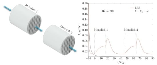
Figure 4 shows the contour plots for k at Re = 100, 200 and 300 along the domain from LES. The figure shows only the first channel and the open space before and after it (−10 $\le Z/D_H\le$ 47). k, which is computed according to (5), comes from the highly turbulent upstream flow that rapidly decreases in the open section, not even reaching the entrance of the first channel in the three analyzed Re values. A noticeable difference between the three cases is that unsteadiness seems to decay almost completely for Re = 100, while for Re = 300, it propagates backwards, affecting a large part of the channel. Fluctuations are assumed to be laminar because of the subcritical channel Re, which means that any turbulence triggered locally should dissipate quickly [23]. As expected, this result is corroborated by LES results showing that the flow in the channels does not remain steady along of the channels and when leaving them. On the other hand, k-$k_L$-$\omega$ predicts a similar decay of the turbulence from the inlet and along of the open section (see Figure 5). Despite the fact that the decay pattern in that region seems more diffusive than that from LES, especially as Re increases, the agreement between the models is acceptable. In the rest of the domain, the k-$k_L$-$\omega$ model should be able to consider the non-turbulent transitional fluctuations [39,49], yet it seems to overestimate the damping of the unsteady movement, predicting steady laminar flow across the whole domain after the initial decay, showing that $k_{TOT}$ exhibits no signs of recovery even in the open section between the channels, irrespective of the channel Re. This differs significantly from LES, which shows a significant increase in the value of k for Re = 300 once the flow leaves the channel.

Figure 6 shows k from LES and k-$k_L$-$\omega$ according to Equations (5) and (12), respectively. For both models, the data correspond to a centre line along the domain, but in LES, it represents the time-averaged values. Both lines correspond to a case with Re = 200. The figure allows us to see the differences when predicting the flow transition from both models in more detail. According to k-$k_L$-$\omega$, k effectively progressively decreases to zero and remains at that value for the rest of the domain. Such a value is reached practically at the outlet of Channel 1. It is also noticeable that neither the inlet or outlet of the substrate affects the decay pattern.

In turn, LES shows that k reaches a base value before entering the first channel, then increases at the inlet of the channel. This is expected in a physical system because of the reduction in the flow area when entering a substrate. The velocity along the centre line of the channel continues to rise in a manner similar to that for laminar flow so that k also increases. Next, at the end of the channel, there is a peak of k, which is typically produced because of the detachment of the boundary layer from the end of the channel walls, which decays towards the same base value observed in the open section before the first channel. This pattern repeats almost identically for the second channel.

From the previous results, one can say that k from LES maintains consistency with mass conservation by effectively capturing the impact of the variable mass flow entering the domain; meanwhile, k-$k_L$-$\omega$ is unable to account for the velocity fluctuations in the analyzed scenario, either laminar or turbulent.

3.3. Frequency Analysis of the Velocity Pattern

The Fourier analysis of the instantaneous velocity in the developed zone is shown in Figure 7. It was verified that the frequency spectrum range contained in the flow increases together with Re inside of the channel. Furthermore, the dominant frequency tends to increase in magnitude with higher Re values in the channel, and its range shifts towards a higher frequency value. The concept of dominant frequency is used to identify the frequency with the highest amplitude in the signal [55,56]. However, in this case, the processed signals have large fluctuations with high frequency, i.e., the velocity varies rapidly with respect to the mean flow velocity, resulting in several peaks, as shown in in Figure 7, which makes it difficult to identify the dominant peak. Hence, the analysis was conducted qualitatively.

The power spectrum density (PSD) of the velocity signal in monolithic channels obtained with the Welch method is shown in Figure 8. The analyzed data came from LES and monitoring point 1 (see Figure 2). By extension, provided that, according to Section 3.1, the velocity signals from both channels completely overlap in terms of frequency, the information contained in them is identical, and the analysis presented in this section is equally valid for both channels.

Figure 8 shows that as Re increases, a greater amount is observed to be concentrated in the lower frequencies. For cases of Re = 100 and Re = 200, a trend in the sudden cut is observed in the PSD curves at approximately $1\times {10}^4$ and $2\times {10}^4$, respectively. This usually occurs in the power spectrum of unsteady laminar flows, diverging from the typical PSD of a fully turbulent flow, which has a continuous transition across all scales due to the energy cascade from larger to smaller eddies. For the case of Re = 300 case, such a trend is not observed, since the inverse value of the time step used in the model resolution was higher than the upper limit of the frequency spectrum range for this condition. Therefore, it is recommended to use even smaller time steps when describing the complete frequency spectrum for Re > 200. Under any circumstance, based on the evidence available for the other cases, there is no reason to expect different behaviour for Re = 300.

3.4. Pressure Profile and Back Pressure through the Substrates

Because it is an important design variable, pressure was also analyzed. The dimensionless pressure through the centre line of the domain for all models and all Re values is shown in Figure 9. As in previous comparisons, the time-averaged data were considered. The pressure was non-dimensionalized to avoid scale problems. Despite the significant differences in the velocity pattern between LES and laminar and k-$k_L$-$\omega$ models, the dimensionless static pressure from all models agrees quite well for all the analyzed Re values. It should be noted that in flow-through monoliths, major losses are proportional to U [57], while dimensionless pressure is scaled by $U^2$; hence, the curve corresponding to higher Re values ends at the bottom of the plot, while that for the lower Re values is placed at the top.

Based on Figure 9, both laminar and k-$k_L$-$\omega$ models predict identical pressures, while there are some marginal differences coming from LES. This makes sense because for LES, the time average is used, and the time-averaged velocity for the three models is the same. Additionally, according to Wo, the eventual pulsating regime for the cases analyzed in this paper is in the range in which a parabolic velocity profile is still achieved [58]. The parabola becomes more and less pronounced but maintains its shape; hence, the pressure drop is expected to be similar to that of laminar flow.

Considering the scenario of laminar flow, the static pressure remains constant during the first section of the domain as a result of the flat velocity profile at the inlet and negligible viscous losses in the open section before the substrate. Then, flow collides with the frontal face of the substrate, where the flow area is reduced; as a consequence, there are some non-linear head losses, as expected in flow-through and wall-flow monoliths [59,60,61,62,63]. Inside of Channel 1, the boundary layer develops rapidly, and losses from friction between flow lamina become linear in the fully developed zone. At the rear face of the substrate, the flow area expands; hence, velocity decreases, causing an increase in static pressure. The flow profile becomes flat in the gap between the channels, so there is no friction or losses in that part of the domain. In this study, a flat velocity profile was achieved in the gap before the flow enters Channel 2 for all analyzed cases, provided that the length of the gap was intentionally dimensioned to accomplish such a condition.

Channel 2 repeats the same pattern as that of Channel 1 for all tested Re values. For each Re, the pressure drop and entrance length are also the same for both channels.

A final analysis was performed, comparing the total back pressure predicted by the different models as shown in Figure 10. Consistent with previously reported data, where pressure measurements along the center line are identical, the total back pressure predicted for all three models exhibits close similarity across the range of studied Re values, in agreement with previous studies of domains under similar circumstances [64,65,66]. The LES model estimates a slightly smaller pressure drop than when assuming a steady laminar regime. As described in previous comparable studies [24,33], an unsteady laminar flow characterized by multiple pulsation frequencies in monolithic channels shows a negligible impact on pressure drop.

4. Conclusions

The transition of the flow regime through two monoliths in series was successfully studied by means of a computational model at the channel scale.

According to the results, there is no difference in flow behaviour between the two in-series monolith channels. As a result, the sequential channels can be regarded as an extension of the initial channel, requiring only knowledge of the inlet boundary conditions for the first channel to model the other monoliths in series. Such an assumption significantly reduces the needed computational resources to predict the performance of an array of monoliths.

Frequency analysis indicates that there is no turbulence inside of the first channel nor in the downstream channel. The flow inside of the monolith channels seems unsteady and laminar, and despite not being a single-frequency pulsation, it has the features of a pulsating flow where the back pressure is the same as that from steady laminar flow when taking the time-averaged condition as a reference.

An increase in the amplitude of the unsteady velocity fluctuations is observed when the flow leaves the first channel; however, it does not affect the second channel, provided that the gap between them is sufficient to diminish them to the base level shown before entering the first channel. The pulsations resulting from the decay of turbulence inside of the channels do not promote turbulence.

The transitional k-$k_L$-$\omega$ model is not able to accurately describe the transition of the flow regime inside of the monolith channels predicted by LES. According to the RANS model, both turbulence and laminar fluctuations decay to zero inside of the substrate and are unaffected by the change in the flow area when entering and leaving a substrate.

References

- Kapteijn, F.; Moulijn, J.A. Structured catalysts and reactors–Perspectives for demanding applications. Catal. Today 2022, 383, 5–14. [Google Scholar] [CrossRef]
- Vermeiren, W.; Gilson, J.P. Impact of zeolites on the petroleum and petrochemical industry. Top. Catal. 2009, 52, 1131–1161. [Google Scholar] [CrossRef]
- Salamon, E.; Cornejo, I.; Mmbaga, J.P.; Kołodziej, A.; Lojewska, J.; Hayes, R.E. Investigations of a three channel autogenous reactor for lean methane combustion. Chem. Eng. Process.-Process Intensif. 2020, 153, 107956. [Google Scholar] [CrossRef]
- Önsan, Z.I.; Avci, A.K. Multiphase Catalytic Reactors: Theory, Design, Manufacturing, and Applications; John Wiley & Sons: Hoboken, NJ, USA, 2016. [Google Scholar]
- Xu, X.; Moulijn, J.A. Transformation of a structured carrier into structured catalyst. In Structured Catalysis and Reactors; Marcel Dekker: New City, NY, USA, 1998; pp. 599–616. [Google Scholar]
- Heck, R.M.; Gulati, S.; Farrauto, R.J. The application of monoliths for gas phase catalytic reactions. Chem. Eng. J. 2001, 82, 149–156. [Google Scholar] [CrossRef]
- Schutt, B.D.; Abraham, M.A. Evaluation of a monolith reactor for the catalytic wet oxidation of cellulose. Chem. Eng. J. 2004, 103, 77–88. [Google Scholar] [CrossRef]
- Holmgren, A.; Gronstedt, T.; Andersson, B. Improved flow distribution in automotive monolithic converters. React. Kinet. Catal. Lett. 1997, 60, 363–371. [Google Scholar] [CrossRef]
- Heibel, A.; Spaid, M.A. A New Converter Concept Providing Improved Flow Distribution and Space Utilization; SAE Technical Paper 1999-01-0768; SAE International: Warrendale, PA, USA, 1999. [Google Scholar] [CrossRef]
- Reinao, C.; Cornejo, I. A Model for the Flow Distribution in Dual Cell Density Monoliths. Processes 2023, 11, 827. [Google Scholar] [CrossRef]
- Cornejo, I.; Garreton, G.; Hayes, R.E. On the use of dual cell density monoliths. Catalysts 2021, 11, 1075. [Google Scholar] [CrossRef]
- Arab, S.; Commenge, J.M.; Portha, J.F.; Falk, L. Methanol synthesis from CO2 and H2 in multi-tubular fixed-bed reactor and multi-tubular reactor filled with monoliths. Chem. Eng. Res. Des. 2014, 92, 2598–2608. [Google Scholar] [CrossRef]
- Williams, J.L. Monolith structures, materials, properties and uses. Catal. Today 2001, 69, 3–9. [Google Scholar] [CrossRef]
- Cristiani, C.; Visconti, C.G.; Finocchio, E.; Stampino, P.G.; Forzatti, P. Towards the rationalization of the washcoating process conditions. Catal. Today 2009, 147, S24–S29. [Google Scholar] [CrossRef]
- Banús, E.; Ulla, M.; Miró, E.; Milt, V. Structured catalysts for soot combustion for diesel engines. Chapter 2013, 5, 117–142. [Google Scholar]
- Hayes, R.; Liu, B.; Moxom, R.; Votsmeier, M. The effect of washcoat geometry on mass transfer in monolith reactors. Chem. Eng. Sci. 2004, 59, 3169–3181. [Google Scholar] [CrossRef]
- Cornejo, I.; Hayes, R.E. A review of the critical aspects in the multi-scale modelling of structured catalytic reactors. Catalysts 2021, 11, 89. [Google Scholar] [CrossRef]
- Chanda Nagarajan, P.; Ström, H.; Sjöblom, J. Numerical Assessment of Flow Pulsation Effects on Reactant Conversion in Automotive Monolithic Reactors. Catalysts 2022, 12, 613. [Google Scholar] [CrossRef]
- Cornejo, I.; Nikrityuk, P.; Hayes, R.E. Heat and mass transfer inside of a monolith honeycomb: From channel to full size reactor scale. Catal. Today 2022, 383, 110–122. [Google Scholar] [CrossRef]
- Schardt, S.; Celik, A.; Chawla, J.; Bastian, S.; Schunk, S.A.; Lott, P.; Deutschmann, O. Pt-Based Monolithic Catalysts for Oxidative Coupling of Methane: Effect of Catalyst Formulation and Operation Parameters. In Proceedings of the 2022 AIChE Annual Meeting, Phoenix, AZ, USA, 13–18 November 2022. [Google Scholar]
- Cornejo, I.; Nikrityuk, P.; Hayes, R.E. Improved Nu number correlations for gas flow in monolith reactors using temperature-dependent fluid properties. Int. J. Therm. Sci. 2020, 155, 106419. [Google Scholar] [CrossRef]
- Cornejo, I.; Nikrityuk, P.; Hayes, R.E. Turbulence decay inside the channels of an automotive catalytic converter monolith. Emiss. Control. Sci. Technol. 2017, 3, 302–309. [Google Scholar] [CrossRef]
- Cornejo, I.; Cornejo, G.; Nikrityuk, P.; Hayes, R.E. Entry length convective heat transfer in a monolith: The effect of upstream turbulence. Int. J. Therm. Sci. 2019, 138, 235–246. [Google Scholar] [CrossRef]
- Cornejo, I.; Nikrityuk, P.; Lange, C.; Hayes, R.E. Influence of upstream turbulence on the pressure drop inside a monolith. Chem. Eng. Process.-Process Intensif. 2020, 147, 107735. [Google Scholar] [CrossRef]
- Hettel, M.; Daymo, E.; Schmidt, T.; Deutschmann, O. CFD-Modeling of Fluid Domains with Embedded Monoliths with Emphasis on Automotive Converters. Chem. Eng. Process. Process Intensif. 2019, 147, 107728. [Google Scholar] [CrossRef]
- Cornejo, I.; Nikrityuk, P.; Hayes, R.E. Multiscale RANS-based modeling of the turbulence decay inside of an automotive catalytic converter. Chem. Eng. Sci. 2018, 175, 377–386. [Google Scholar] [CrossRef]
- Cornejo, I.; Nikrityuk, P.; Hayes, R.E. Turbulence generation after a monolith in automotive catalytic converters. Chem. Eng. Sci. 2018, 187, 107–116. [Google Scholar] [CrossRef]
- Cornejo, I.; Nikrityuk, P.; Hayes, R.E. Effect of substrate geometry and flow condition on the turbulence generation after a monolith. Can. J. Chem. Eng. 2020, 98, 947–956. [Google Scholar] [CrossRef]
- Nagarajan, P.C.; Larsson, J.; Tylén, O.; Murali, A.; Larsson, A.; Peyvandi, E.; Rangaswamy, S.; Ström, H.; Sjöblom, J. Turbulent uniformity fluctuations in automotive catalysts–A RANS vs DES assessment. Results Eng. 2022, 16, 100772. [Google Scholar] [CrossRef]
- Cornejo, I.; Hayes, R.E.; Nikrityuk, P. A new approach for the modeling of turbulent flows in automotive catalytic converters. Chem. Eng. Res. Des. 2018, 140, 308–319. [Google Scholar] [CrossRef]
- Tikekar, M.; Singh, S.G.; Agrawal, A. Measurement and modeling of pulsatile flow in microchannel. Microfluid. Nanofluidics 2010, 9, 1225–1240. [Google Scholar] [CrossRef]
- Benjamin, S.; Zhao, H.; Arias-Garcia, A. Predicting the flow field inside a close-coupled catalyst—The effect of entrance losses. Proc. Inst. Mech. Eng. Part C J. Mech. Eng. Sci. 2003, 217, 283–288. [Google Scholar] [CrossRef]
- Cornejo, I. A Model for Correcting the Pressure Drop between Two Monoliths. Catalysts 2021, 11, 1314. [Google Scholar] [CrossRef]
- Hayes, R.E.; Cornejo, I. Multi-scale modelling of monolith reactors: A 30-year perspective from 1990 to 2020. Can. J. Chem. Eng. 2021, 99, 2589–2606. [Google Scholar] [CrossRef]
- White, F.M. Fluid Mechanics; McGraw-Hill: New York, NY, USA, 2009. [Google Scholar]
- Bertrand, F.; Devals, C.; Vidal, D.; de Préval, C.S.; Hayes, R.E. Towards the simulation of the catalytic monolith converter using discrete channel-scale models. Catal. Today 2012, 188, 80–86. [Google Scholar] [CrossRef]
- Wilcox, D.C. Reassessment of the scale-determining equation for advanced turbulence models. AIAA J. 1988, 26, 1299–1310. [Google Scholar] [CrossRef]
- Wilcox, D.C. Turbulence Modeling for CFD; DCW Industries: La Canada, CA, USA, 1993. [Google Scholar]
- Walters, D.K.; Cokljat, D. A three-equation eddy-viscosity model for Reynolds-averaged Navier–Stokes simulations of transitional flow. J. Fluid. Eng. 2008, 130, 121401. Available online: www.ansys.com (accessed on 3 May 2023). [CrossRef]
- ANSYS. ANSYS® Academic Research, Release 2022R2, Ansys Fluent, Theory Guide; ANSYS: Canonsburg, PA, USA, 2022. [Google Scholar]
- Yang, L.; Yu, Y.; Pei, H.; Gao, Y.; Hou, G. Lattice Boltzmann simulations of liquid flows in microchannel with an improved slip boundary condition. Chem. Eng. Sci. 2019, 202, 105–117. [Google Scholar] [CrossRef]
- Rahman, M.E.; Weibel, J.A. Mapping the amplitude and frequency of pressure drop oscillations via a transient numerical model to assess their severity during microchannel flow boiling. Int. J. Heat Mass Transf. 2022, 194, 123065. [Google Scholar] [CrossRef]
- Kim, W.W.; Menon, S.; Kim, W.W.; Menon, S. Application of the localized dynamic subgrid-scale model to turbulent wall-bounded flows. In Proceedings of the 35th Aerospace Sciences Meeting and Exhibit, Reno, NV, USA, 6–9 January 1997; p. 210. [Google Scholar]
- Menon, S.; Yeung, P.K.; Kim, W.W. Effect of subgrid models on the computed interscale energy transfer in isotropic turbulence. Comput. Fluid. 1996, 25, 165–180. [Google Scholar] [CrossRef]
- Menon, S.; Kim, W.W. High Reynolds number flow simulations using the localized dynamic subgrid-scale model. In Proceedings of the 34th Aerospace Sciences Meeting and Exhibit, Reno, NV, USA, 15–18 January 1996; p. 425. [Google Scholar]
- Hanjalić, K.; Launder, B. Eddy-viscosity transport modelling: A historical review. In 50 Years of CFD in Engineering Sciences: A Commemorative Volume in Memory of D. Brian Spalding; Springer: Singapore, 2020; pp. 295–316. [Google Scholar]
- Malalasekera, W.; Versteeg, H. An Introduction to Computational Fluid Dynamics: The Finite Volume Method; PEARSON Prentice Hall: Upper Saddle River, NJ, USA, 2007. [Google Scholar]
- Menter, F. Two-equation eddy-viscosity turbulence models for engineering applications. AIAA J. 1994, 32, 1598–1605. [Google Scholar] [CrossRef]
- Walters, D.K.; Leylek, J.H. A new model for boundary layer transition using a single-point RANS approach. J. Turbomach. 2004, 126, 193–202. [Google Scholar] [CrossRef]
- Patankar, S. Numerical Heat Transfer and Fluid Flow; CRC Press: Boca Raton, FL, USA, 1980. [Google Scholar]
- ANSYS Fluent Software Package v2022R2; ANSYS Inc.: Canonsburg, PA, USA, 2022.
- Leishman, J.G. Internal Fluid Flows. In Introduction to Aerospace Flight Vehicles; Eagle Pubs: Daytona Beach, FL, USA, 2023. [Google Scholar]
- Shah, R.K.; London, A.L. Laminar Flow Forced Convection in Ducts: A Source Book for Compact Heat Exchanger Analytical Data; Academic Press: Cambridge, MA, USA, 2014. [Google Scholar]
- Du Plessis, J.; Collins, M. A new definition for laminar flow entrance lengths of straight ducts. N&O J. 1992, 25, 11–16. [Google Scholar]
- Mitra, S.K. Digital Signal Processing: A Computer-Based Approach; McGraw-Hill Higher Education: New York, NY, USA, 2001. [Google Scholar]
- Everett, T.H.; Kok, L.C.; Vaughn, R.H.; Moorman, R.; Haines, D.E. Frequency domain algorithm for quantifying atrial fibrillation organization to increase defibrillation efficacy. IEEE Trans. Biomed. Eng. 2001, 48, 969–978. [Google Scholar] [CrossRef]
- Cornejo, I.; Nikrityuk, P.; Hayes, R.E. Pressure correction for automotive catalytic converters: A multi-zone permeability approach. Chem. Eng. Res. Des. 2019, 147, 232–243. [Google Scholar] [CrossRef]
- Zamir, M.; Zamir, M. Pulsatile flow in an elastic tube. In The Physics of Pulsatile Flow; Springer: New York, NY, USA, 2000; pp. 113–145. [Google Scholar]
- Clarkson, R.J. A Theoretical and Experimental Study of Automotive Catalytic Converters. Ph.D. Thesis, Coventry University, Coventry, UK, 1997. [Google Scholar]
- Ekström, F.; Andersson, B. Pressure drop of monolithic catalytic converters experiments and modeling. SAE Tech. Pap. 2002, 111, 425–433. [Google Scholar]
- Mesquida, I.M.V.; Cornejo, I.; Nikrityuk, P.; Greiner, R.; Votsmeier, M.; Hayes, R.E. Towards a fully predictive multi-scale pressure drop model for a wall-flow filter. Chem. Eng. Res. Des. 2020, 164, 261–280. [Google Scholar] [CrossRef]
- Wang, W.; Bissett, E.J. Frictional and Heat Transfer Characteristics of Flow in Triangle and Hexagon Channels of Wall-Flow Monoliths. Emiss. Control. Sci. Technol. 2018, 4, 198–218. [Google Scholar] [CrossRef]
- Watling, T.C. A One-Dimensional Model for Square and Octo-Square Asymmetric Particulate Filters with Correct Description of the Channel and Wall Geometry; SAE Technical Paper 2018-01-0951; SAE International: Warrendale, PA, USA, 2018. [Google Scholar] [CrossRef]
- Dutta, P.; Nandi, N. Study on pressure drop characteristics of single phase turbulent flow in pipe bend for high Reynolds number. ARPN J. Eng. Appl. Sci. 2015, 10, 2221–2226. [Google Scholar]
- Seeley, B.D.; Young, D.F. Effect of geometry on pressure losses across models of arterial stenoses. J. Biomech. 1976, 9, 439–448. [Google Scholar] [CrossRef] [PubMed]
- Akbarzadeh, M.; Rashidi, S.; Esfahani, J. Influences of corrugation profiles on entropy generation, heat transfer, pressure drop, and performance in a wavy channel. Appl. Therm. Eng. 2017, 116, 278–291. [Google Scholar] [CrossRef]
Figure 1.
Schematic representation of the elements of the reactor, from the full-scale reactor (a) to a honeycomb channel cross-section showing the wash-coat layer in light brown (e). Adapted from [17].
Figure 2.
Computational domain for two monolith channels placed in series.
Figure 3.
Dimensionless velocity through time at = 15 from the inlet of both channels.
Figure 4.
k (m/s) contour for all studied Re conditions from LES.
Figure 5.
(m/s) contour for all studied Re conditions from k--.
Figure 6.
Kinetic energy predicted by LES and k-- over the axis of the domain.
Figure 7.
Frequency spectrum for all studied Re values.
Figure 8.
Power spectrum for all studied Re values.
Figure 9.
Pressure through the centre-line monolith channels.
Figure 10.
Back pressure for different Re values.