A Data-Driven Surrogate Approach for the Temporal Stability Forecasting of Vegetation Covered Dikes


1
Geoscience & Engineering Department, Faculty of Civil Engineering and Geosciences, Delft University of Technology, 2628 CN Delft, The Netherlands
2
Unit Geo-Engineering, Deltares, 2629 HV Delft, The Netherlands
3
Geoscience & Remote Sensing Department, Faculty of Civil Engineering and Geosciences, Delft University of Technology, 2628 CN Delft, The Netherlands
*
Author to whom correspondence should be addressed.
Water 2021, 13(1), 107; https://doi.org/10.3390/w13010107
Submission received: 1 December 2020
/
Revised: 27 December 2020
/
Accepted: 29 December 2020
/
Published: 5 January 2021
(This article belongs to the Special Issue Water-Induced Landslides: Prediction and Control)
Abstract
:Climatic conditions and vegetation cover influence water flux in a dike, and potentially the dike stability. A comprehensive numerical simulation is computationally too expensive to be used for the near real-time analysis of a dike network. Therefore, this study investigates a random forest (RF) regressor to build a data-driven surrogate for a numerical model to forecast the temporal macro-stability of dikes. To that end, daily inputs and outputs of a ten-year coupled numerical simulation of an idealised dike (2009–2019) are used to create a synthetic data set, comprising features that can be observed from a dike surface, with the calculated factor of safety (FoS) as the target variable. The data set before 2018 is split into training and testing sets to build and train the RF. The predicted FoS is strongly correlated with the numerical FoS for data that belong to the test set (before 2018). However, the trained model shows lower performance for data in the evaluation set (after 2018) if further surface cracking occurs. This proof-of-concept shows that a data-driven surrogate can be used to determine dike stability for conditions similar to the training data, which could be used to identify vulnerable locations in a dike network for further examination.
1. Introduction
Dikes and embankments are important geo-structures that provide protection against inundation or flooding [1]. In the Netherlands, dikes form a large part of the existing flood defence systems, with a total length of about 18,000 km, of which 14,000 km are regional (secondary) dikes. Therefore, the continuous assessment of dikes is one of the main challenges that civil works managers and geotechnical engineers are dealing with in the Netherlands [2,3,4]. This is primarily due to the fact that the failure of these geo-structures, like other engineered and natural slopes, may have significant economic, social and environmental consequences [5]. Therefore, the timely analysis and prediction of stability of these slopes allow decision makers to adopt appropriate measures to minimise the risk of slope failure in hazard-prone areas.
Rainfall-induced slope failure typically happens due to the reduction of the matric suction near the slope surface and/or elevated ground water level that leads to an increase in pore water pressure (pwp) and a decrease in effective stress. Hence, the reduction of the shear resistance of the soil, and an increase in the weight of the slope, increase shear stress on the soil. Depending on the type of slope and the scale of the analysis, different methods are used for slope stability assessment.
In the context of natural slopes, where landslide forecasting is the main goal, these methods target both spatial and temporal forecasting. They range from data-driven approaches such as statistics-based methods which are typically used for regional to global slope stability analysis [6,7], to simplified physics-based methods often used on a local scale (e.g., infinite slope analysis [8,9,10]) and advanced numerical analysis methods such as the finite element method (FEM) at the site-specific scale [11].
For engineered slopes, physics-based numerical and analytical methods prevail due to the higher accuracy of these approaches, and the typical high consequence of their failure. Physics-based models, however, require a broad range of geotechnical and hydro-geomechanical in situ data for the accurate estimation of the state of individual slopes. Although in situ data are typically available for the analysis of engineered slopes, practically speaking, it is impossible to have accurate slope data with very high spatial and temporal resolutions and coverage. This results in considerable uncertainty on the inputs and outputs of numerical models for analysing slope stability. Moreover, analysing the transient stability of slopes is usually computationally expensive, such that real-time simulations are virtually impossible, especially if incorporating climatic data or calibrated to observed data. Therefore, an efficient approach for slope stability prediction can provide a quick estimation of the slope condition and hence speed up the assessment process. Data-driven approaches, such as machine learning (ML), have the potential to fulfil this purpose. ML algorithms have been used at the regional scale to estimate slope stability. The majority of work on landslide susceptibility mapping uses variants of ML algorithms (e.g., [12,13,14,15,16,17,18,19,20,21]). In these studies, historical slope failures were linked with associated pre-disposing factors such as terrain features, landcover, and shallow lithology to derive a pattern (model) that link these factors to the occurrence of landslides.
In recent years, static susceptibility maps have been combined with dynamic data for forecasting rainfall-induced landslides (e.g., [22,23,24,25,26]). For instance, Segoni et al. [27] used a susceptibility model, constructed using random forest (RF) classification, rainfall measurements and empirical rainfall thresholds to predict potential rainfall-induced landslides in northern Italy. A similar approach has been used for landslide ‘now-casting’ at the global level [25].
Recently, several studies have employed data-driven methods for evaluating the stability of slopes [28]. Wei et al. [29] used historical rainfall records and pwp measurements from a slope in Hong Kong to train ML-based prediction models. Chakraborty and Goswami [30] estimated the factor of safety (FoS) of 110 slopes with different geometric and shear strength parameters using ML. They compared the obtained results with a finite element (FE) model, and an acceptable rate of accuracy was observed for the predicted FoS. Pei et al. [31] used RF and regression tree predictive models in soil-landscape modeling for predicting the depth of the failure plane on a regional basis. They developed a classification for detecting the safe and hazardous slopes by means of FoS calculations. Qi et al. [32] used different ML classification algorithms including RF (with the highest accuracy among all models) to forecast the slope stability for 148 slopes, using geometric characteristics (slope angle and height) and soil parameters (cohesion, internal friction angle and unit weight). While these studies were successful in identifying vulnerable slopes, temporal changes in the FoS were not identified. Among the different algorithms used in predicting slope stability conditions, ensemble tree-based methods such as RF classifiers and regressors proved to be promising [6,7,32,33]. These methods are known to be robust against over-fitting, in which case the model performs well on training data, but performs poorly on the test set. Moreover, as the number of trees increases, the generalisation error (a measure for the algorithm accuracy in predicting target values/class for previously unseen data) converges to a limit [34].
While static slope parameters (e.g., layering, cohesion, internal friction angle and unit weight) can be measured, a high degree of accuracy at the regional scale is challenging, and temporal changes (e.g., degree of saturation, suction, bulk density) are generally neither known nor feasible to measure at the regional scale, without cost-prohibitive extensive monitoring. Continuous analysis and prediction of dike stability (and any other slope stability), however, is not possible without proper physical inspection and monitoring. This is because the slope failure is a time-dependent process that causes the deterioration or damage of slope components and ultimately leads to failure [3]. Periodic inspections are often used to assess the overall condition of dike systems, and detect vulnerable areas, which generally use surface conditions, e.g., cracks and vegetation, to imply the dike condition. Dike inspection procedures, regulations and processes (e.g., frequency and criteria) vary between countries [1]. There are in situ monitoring systems, such as electrical resistivity tomography, by which the dike condition can be assessed through, for instance, crack openings and water infiltration [35]. In the Netherlands, the current monitoring methods of dikes usually consist of infrequent (typically twice per year for regional dikes [36]) ground-based visual inspections, which rely highly on expert judgement. Thanks to (low cost or free) satellite images that have become available in recent years, there is a potential to use large (global) data sets to inspect slopes from space. For instance, vegetation indices (VIs) are accessible through both optical and radar remote sensing, and surface displacement can be measured with the interferometric synthetic aperture radar (InSAR) techniques [37,38]. InSAR deformation/displacement analysis techniques provide surface deformation with high spatial and temporal resolution, e.g., 5 m by 20 m at every 6 day repeat cycle for the Sentinel-1 satellite [39]. InSAR techniques have been shown to be able to quantify the movements of unstable slopes, and it has been shown to be highly effective in mapping slow landslides [40].
Our recent studies [36,41] show that transient surface displacement and vegetation condition have strong correlations with the slope FoS, due to their correlation with the moisture content of the slope. In those numerical studies, the meteorological data combined with soil parameters were used as input for the model to estimate the change in FoS and the non-linear hydro-mechanical behaviour of a dike under various weather and vegetation conditions. The results were qualitatively validated using in situ data from an instrumented dike [42]. The same temporal signature and strong correlation in key parameters were observed in the real dike. As both the transient surface displacement and vegetation condition are observable features, they can be used for dike inspection, and for calculating the FoS to predict the macro stability of dikes.
In this study, we present a proof-of-concept that a data-driven approach can be used to emulate expensive numerical simulations, to calculate the factor of safety of dikes utilising only Earth observation (EO) data. First, the slope surface parameters most closely related to the FoS are identified. These parameters, together with results from a detailed numerical model, are then used to train an RF regression model to predict the slope stability state. Results of the prediction models are validated with the calculated FoS from the numerical simulations to evaluate the performance of the data-driven method. The factor of safety (or other measures of safety) are not measurable quantities, and even dike failure would also be a single data point, i.e., the factor of safety would be known to be below 1. Therefore, the step towards validation of the method with field data has not been made. However, numerical models have been substantially validated (e.g., [43]); therefore, such a model is used here to trial our proof-of-concept model. This research aims to investigate if data-driven methods can be applied to assess a dike condition using EO data, which is not currently used in monitoring vegetation covered dikes. To the authors’ knowledge, this is the first time that data-driven methods have been applied to dike stability calculations, only considering parameters which can be obtained from EO and the first time in which vegetation and climatic conditions have been considered. Therefore, one illustrative case study is utilised to show the application of this methodology, highlighting its potential strengths and limitations.
2. Method
Recently, an integrated crop-geotechnical model has been proposed by the authors of this paper for the numerical simulation of dikes and dike FoS to account for hydro-meteorological conditions and the influence of vegetation [36,41]. Here, the same model is used to provide detailed hydro-geomechanical and safety analysis of an idealised dike in order to create a 10-year-long time series of synthetic data of the dike behaviour. These results are analysed to identify the observable features of the model that have the strongest influence on FoS. As the intention here is to estimate the transient FoS from the dike surface, only superficial transient features are investigated. The features are used to train an RF algorithm to predict the stability/safety of the dike.
2.1. Integrated Crop-Geotechnical Model
Commonly used geotechnical models (e.g., PLAXIS [44]) do not simulate the dynamic effects of vegetation on water flux (evaporation and influx) and therefore do not consider the influence that vegetation may have on land–atmosphere interactions and slope stability. Crop models, however, have been used to simulate the interaction of vegetation and the upper soil layers (e.g., LINGRA [45]). In recent research [36], the two models (LINGRA and PLAXIS) were coupled together to assess the effect of variable climatic and vegetation conditions on dike stability. As evaporation-induced cracks alter the water balance in a dike by increasing flow through the cracks and at the same time reducing the shear strength of the root zone, the model was further modified to include the effect of surface cracks [41]. Here, it is assumed that the cracks do not seal (close) in the wet periods, but only expand during unprecedented dry conditions. For example, if a crack is developed when root zone soil moisture () is 0.2 (cm water cm soil), it will expand when SM drops below 0.2. However, the crack area does not change if SM reverts above 0.2. The key inputs and outputs of the model are shown in Figure 1, where is the leaf area index, is the percentage of the crack area and GWL is the ground water level. The outputs are explained further in Section 3.1. In this paper, a 2D model of a vegetated dike is built using the integrated crop-geotechnical model and used to provide synthetic data.
2.2. Machine Learning Method
The synthetic data set, from the integrated crop-geotechnical model, is used to build and train an RF algorithm to predict the safety/stability condition (i.e., FoS) of the vegetated dike. The main idea here is to estimate the stability of the dike, without repeating expensive numerical simulations, using data that can be potentially observed without physical contact measurements. The general procedure for the ML model in this research is shown in Figure 2. The input features of the RF model include rain and temperature values obtained from the meteorological data, as well as and displacement, which are readily observable using remote sensing. The chosen parameters are also those with the highest impact on the target value, i.e., the FoS. For instance, rain and air temperature have a higher influence on FoS rather than other meteorological parameters used in the numerical study. In addition, the importance of as an input feature is investigated, as it is in theory observable from the dike surface, but there are no methods to do so yet available. The target (output) variables of the RF model are the FoS values predicted by the numerical model. The temporal resolution is 1 day for all of the features; , and are averaged over the surface. Displacement is retrieved for one location (one point) on the surface. The target value, FoS, is considered for the whole dike geometry.
2.2.1. Random Forest Algorithm
The random forest (RF) method, which was introduced by Breiman [34], is an ensemble learning method used for classification and regression. The RF algorithm is based on an ensemble of decision trees (DT) for classification or regression trees (RT) for regression. In this study, we use RTs, since the target outputs are quantities (not classes) that need to be predicted. The Python library ‘Scikit-learn’ [47] has been used here for the RF regression analysis.
The RF is a series of tree-like graphs, as shown schematically in Figure 3. A decision/regression tree (DT/RT) is a set of decision boundaries (yes/no questions or thresholds) regarding every feature in the training data that eventually leads to a predicted class or value for classification or regression, respectively. For regression, this threshold is obtained by scanning through all the values of that feature in the training data and finding the threshold (called the optimal threshold here) that results in the minimum sum of square of the difference between the predicted target value and the actual target value. A root node is the entry node on top of the RT, where a first decision boundary is set by asking if the first selected feature (can be any feature in the context of random forest) is less than or greater than an optimal threshold. This action divides the data into smaller subsets, where the action is repeated for other features (intermediate nodes) and the tree is expanded until the decision is made about the target value in the last node (leaf node). More information on DTs can be found in [48].
For regression, RF builds a number of regression trees (N) and the final predicted values are obtained by the aggregation of the results of all individual trees. The random forests regression predictor is described by the following equation [50]:
where l is the output, in this case the FoS, x is the input vectors for the RF model, n denotes the tree number and N is the number of regression trees in the forest.
Compared to other tree-based algorithms, e.g., those constructed based on boosting (e.g., XGboost), RF is less affected by noise and can generalise better. This improves the stability and accuracy of the model, reduces variance and helps to avoid over-fitting. In addition, RF has fewer parameters (known as hyper-parameters) to tune, and it is easier to visualise and understand. Hastie et al. [51] show that RFs do remarkably well, with very little tuning required compared to other tree-based models. One of the limitations of RF regressors, similar to many other ML algorithms, is that they are not able to extrapolate. In other words, the range of predictions an RF can make is bound by the highest and lowest target and feature values in the training set.
2.2.2. Building and Training the RF Model
The data set, including features and corresponding target values, is divided into training and test sets. During training, each tree in the RF ‘sees’ the answers, and can learn how to predict the target from the features. The RF model learns the relationship between features and the target in training. When testing, the RF is asked to make predictions based on features in a test set. Finally, the model performance is evaluated by comparing the predicted target values and actual values in the test set.
The RF building and learning algorithm has several hyper-parameters (HPs) that have to be defined by the user. For example, the number of observations drawn randomly for each tree, the number of features drawn randomly for each split (branch), the splitting rule, the minimum number of samples that a node must contain, and the number of trees must be defined.
The basic steps for forming a RF algorithm are (after [51]):
- A section of training data (with replacement) is selected. This is made up of a number of samples (the full set of observable features associated with each time point).
- For each selection, a regression tree is constructed, constrained by the user-defined hyper-parameters. At each node, a threshold is determined for a single (randomly selected) feature. The data are then partitioned until a best estimate of the output is calculated.
- The target value from every decision tree is predicted.
- Voting of predicted results is conducted to achieve the terminal predicted results. In a regression RF, voting means using the mean value of results.
In ML, tuning refers to the task of finding the optimal HPs from candidate hyper-parameters for a considered data set [52], that results in best performance. Here, k-fold cross validation [53] is used, as it is one of the most common methods of hyper-parameter tuning. The data in the training set are randomly divided into K roughly equal-sized groups. For the kth group, the model is then trained over the remaining groups. Then, the prediction error of the fitted model on the kth group is calculated. This iteration is repeated K times and the prediction errors are averaged. This cross-validation procedure provides more reliable results as the variance of the estimation is reduced [51].
2.2.3. Feature Importance
It is useful to know the relative importance or relevance of each feature (input variable) to the predicted response (target variable). This helps the user to understand the important drivers for RF to reach its prediction.
In each tree from an RF model, every node implements a condition on a single feature. In other words, that feature is used to make a decision on how to divide the data set into two separate sets (e.g., feature in Figure 3) which have similar responses. The features for nodes in regression trees are selected based on variance reduction in ‘impurity’. Impurity is a measure of how badly the target data (here FoS) at a given node fits the built model. During the training of a regression tree, it can be computed how much each feature decreases the impurity by variance reduction in a tree. For a forest, the ‘impurity’ decrease from each feature can be averaged across the forest and the features are ranked according to this measure. In this study, the RF regressor calculates variance reduction using the mean squared error (MSE) to measure the quality of a split (selecting the optimal value) in intermediate nodes [47].
2.3. Case Study
2.3.1. Numerical Model
An example dike geometry is used in the numerical study which, to a large extent, resembles a regional (secondary) dike in Amsterdam, the Netherlands [2]. The same example dike is also used in [36,41,42]. This dike (Figure 4) has a relatively steep slope on the left-hand side and a gentle slope on the right-hand side and is permanently covered by grass. The dike body has the width of 41 m with a maximum height of 2 m. The dike is founded on a 2.5 m foundation layer of organic clay material, underlain by an impermeable material, represented as an impermeable boundary in Figure 4. The soil surface boundary and the left and right boundaries of the model dike are assumed to be permeable. The vegetation extends over the entire surface of the dike, and is assumed to have a fixed root depth of 40 cm, indicated in green in Figure 4. The dike is subjected to climate-driven forces acting on the surface, i.e., the precipitation, air temperature, wind and solar radiation.
Since the objective of this study is to link climatic data to dike safety, a 10-year meteorological data set from 2009 to 2019 is used. The data were obtained from the The Royal Netherlands Meteorological Institute (KNMI) station at Schiphol Airport (Amsterdam) with global (WGS84) coordinates of (Latitude: 52.31, Longitude: 4.78). In Figure 5a–d, the precipitation, average air temperature, wind speed and solar radiation for the 10-year study period are shown.
The soil and vegetation input parameters for the model are listed in Table 1. The following parameters are used in the crop sub-model. The volumetric water content at the field capacity () is the maximum water storage capacity of the root zone at a suction of 10 kPa or [54] for the soil at initial (intact) conditions. The volumetric water content at the wilting point () is the water content below which plant water uptake ceases and wilting starts. The critical volumetric water content () is the threshold below which transpiration is reduced due to water stress. The maximum drainage rate () of the subsoil is the rate above which the drainage from the root zone to lower layers is limited. The vegetation parameters of the crop sub-model include: the specific leaf area (), which is the leaf area over leaf mass; the remaining after mowing (); and the critical leaf area (), the value beyond which death due to self-shading occurs [55]. The values used for the soil and vegetation in the crop sub-model are based on reported values by [45].
The soil constitutive model parameters (for the Mohr–Coulomb material model), required for the geotechnical sub-model, are based on the soil properties available in the PLAXIS library [44] for the root zone (silty clay) and for the dike body and foundation (organic clay). The selected values for the (Mohr–Coulomb) soil parameters are typical values for materials in the example dike, but are not to be generalised for real cases. The shear strength parameters (c and ) of the root zone are reduced linearly in response to the growth of the crack area . The minimum values of the shear strength parameters are used when the crack area reaches the value . The hydraulic parameters of the root zone are obtained from an optimisation code used to couple the two sub-models [36]. Since the impact of soil cracking is considered in the root zone, the hydraulic properties of the root zone are updated during the analysis for cracked soil.
2.3.2. RF Model
The RFs are built and trained on the synthetic data set generated using the integrated crop-geotechnical model of the example dike. The predictive performance of RF regression is investigated in two scenarios.
- Real-time assessment (RF): the dike safety (FoS) is assessed in real time based on the observable data. The features are selected from the same day on which the FoS is estimated by the RF model.
- Short-term prediction (RF): the dike safety is calculated for some days in the future. This time lag gives dike managers enough time to take necessary actions before the occurrence of potential catastrophic events. All features except rainfall and temperature are for some days prior to the day that FoS is estimated. Rainfall and temperature correspond to the day on which FoS is calculated by the RF model.
In both scenarios, three data sets are formed from the 10-year synthetic data. The data before 2018 will be used for training and testing the RF models: 80% of data are randomly selected as a training set and the remaining 20% as a test set. The data after 2018 are used for independent evaluation of the trained and tested model to check the performance of the trained model on data that it has never ‘experienced’. This set is called the evaluation set, and is useful to explore the generalisation of the model.
RF Model Hyper-Parameters Tuning
To choose the best HPs for the two RF regressors, a 10-fold cross validation (10-CV) was performed on the corresponding training data. The impact of three different values of K (5, 10 and 15) was tested for the RF model. As the influence of the K within this range was found to be negligible, 10-CV was selected for all RF models. The HPs tuned here are as follows: (i) The number of trees in the forest (n-estimator); (ii) The maximum depth of the trees, which is the maximum number of splits until the leaf node; (iii) The min-samples-split which represents the minimum number of samples (observations) in a node which undergoes splitting, this can vary between considering at least one sample at each node to considering all of the samples at each node. When this parameter is increased, each tree in the forest becoming more constrained as it has to consider more samples at each node; (iv) The min-samples-leaf parameter specifies the minimum number of samples required to be at a leaf node. The considered candidates for each hyper-parameter are listed in Table 2; the chosen candidates are within the reasonable range that usually use the RF models.
3. Results and Discussion
3.1. Integrated Crop-Geotechnical Model Simulations
The outputs of the numerical simulations using the integrated crop-geotechnical model are shown in Figure 6. The temporal variation in the crack area is shown in Figure 6a. As mentioned in Section 2.1, it is assumed that cracks do not seal, and that crack formation is therefore irreversible. Most cracking occurs in the first year (2009) after the analysis starts. During wet periods in 2009 (May–August), the crack size remains constant until the next drier period in June 2009. Then, again in the summer of the next two years, the soil experiences the next drier condition, and as a result, cracks expand. The time between cracking events gets longer as the crack expands, only in conditions drier than the previously experienced ones. After 6 years, there is almost no additional cracking until summer 2018, when the driest conditions occurred and reached the maximum value in the studied period. Temporal variations of are shown in Figure 6b. The sudden decrease in on mid-June and mid-August every year is due to mowing events, indicated by vertical dashed lines. These were introduced into the crop model based on the mowing schedule of regional dikes in the Netherlands [36]. In Figure 6c, the change of vegetation growth () in a time window of 15 days is plotted, where (t is the event day). The presence of cracks is seen to decrease the change of vegetation growth after mowing (demonstrated by the ), because less water is available in the root zone. Vegetation can re-grow between mowing events when a substantial amount of rainfall happens in this period (e.g., summer 2014); however, is almost zero when there is a dry period between mowing events (e.g., summer 2018).
The ground water level () measured relative to the base boundary at point A (see Figure 4) is shown in Figure 6e. During wet periods, the water level in the example dike increases, when the soil moisture in the root zone reaches the field capacity. As the spring starts and reduces, the typically decreases and reaches the minimum value in July 2018 when the has the lowest value during the studied period. Figure 6f shows the magnitude of the surface displacement at point A (), which follows a pattern similar to in Figure 6e. The seasonal cycle in is caused by variations in and ; in the winter period, the magnitude of displacement increases, while in the summer, it reduces. A slight accumulation of over time is seen due to plastic displacement and growing cracks due to shrinkage behaviour in the root zone. Finally, the temporal variation of FoS is shown in Figure 6g, which is the result of the combined effect of rainfall, change in and crack area variation from 2009–2019. The maximum crack area, and therefore the minimum shear strength parameter (cohesion and friction angle), lead to a minimum FoS in August 2018 when there is a heavy rainfall event and very low (almost bare soil), due to an extremely dry summer. The results show that the vegetation and dike condition are responsive to the climate condition and there is a similar temporal signature in all the plotted results.
3.2. Correlation between Potential Features and the Factor of Safety
Figure 7 shows the correlation between pairs of FoS and selected features considering a time lag for the simulation data. A positive time lag means that the selected parameters leads the FoS (either positive or negative correlation).
As shown in Figure 7a, the root zone saturation is negatively correlated with the FoS, with the highest correlation at the same day that FoS is calculated. A higher amount of water in the root zone causes a higher pwp, thereby lowering the effective stress and then lowering the stability of the whole dike. This correlation is not strong, since if the root zone experiences very dry conditions, the cracks expand (explained in Section 3.1), which decreases FoS. Although is a good potential indicator for variation of FoS in time, it is not easily observable. Root zone soil moisture could be inferred from surface soil moisture, but cannot be monitored from space unless very long wavelengths are used, which will not be available in the near future [56].
There is a negative correlation between FoS and and represented in Figure 7b,c, respectively. This trend can be seen from the temporal variations in Figure 6e,g. The temporal variation of surface displacement is linked to the variation of water level in the dike. Shrinkage/swelling behaviour of the soil is due to the available water in the soil or ground water level variations, which both affect the dike safety by altering effective stress. Displacement is observable remotely; however, is not, and due to the existing link between these two parameters, monitored displacement can be best used as a feature.
Displacement can be measured with InSAR techniques, currently with a resolution that it cannot be assigned to a specific location on a dike. However, the displacement of the entire dike is highly correlated, as demonstrated by comparing the displacement of two points (point A and point B) in Figure 8. Therefore, having the displacement of any point on a slope is useful.
There is a weak lagged correlation between FoS and or rate of change over 15 days (), shown in Figure 7d,e. The overall correlation is low because vegetation growth is affected by multiple factors including , available energy, and mowing. The presence of vegetation influences stability through water balance. When rainfall occurs, vegetation reduces the amount of water that reaches the dike body; the lower pwp (higher suction) causes higher FoS. On the other hand, as cracks expand, vegetation growth is lower compared to uncracked areas. In rainfall events, preferential flows reach the soil body (more pwp) and shear strength reduces. These factors together lead to a reduction in FoS.
It was also shown that crack presence affected the . Evapotranspiration from the root zone increases due to the crack growth and less water is available for the grass to grow, thereby is reduced as crack area increases. can easily be monitored using space-borne instruments.
Temperature has a weak correlation with FoS (Figure 7f) due to the indirect relation it has on dike stability. In the growing seasons, air temperature is high and vegetation grows. Without rainfall, this causes soil drying, which results in soil cracking and reduction of the . In addition, the air temperature influences the evapotranspiration demand, which influences the variations, already discussed above. The temperature is most strongly correlated with FoS at the maximum time lag considered (30 days) before the FoS. Temperature is measured via existing weather stations, and does not have significant local variations. Therefore, temperature can be used as a feature for an indirect way of assessing the FoS.
The strong negative correlation between crack area and dike safety, shown in Figure 7g, is the consequence of reduction in the shear strength, and preferential flows through the cracks that cause an increase in pwp in the dike body, thereby lowering effective stress and FoS. While the maximum correlation is with a zero time lag, a positive time lag retains a high correlation. Although has a strong correlation with FoS, it is impractical with current methods to measure the crack area.
Rainfall has a negative correlation with FoS mostly with 1 day lag, (Figure 7h), indicating that rain causes a change in FoS after one day, with a low correlation outside of a single day. To consider the effect of antecedent rainfall on dike stability, the correlation between cumulative rainfall with the different time windows and FoS was tested and a 65-day window () (Figure 7i) was found to have the strongest correlation with FoS.
3.3. RF Regression
The results from the previous section are used to build a predictive model. Firstly, an RF is built, tuned and tested using easily observable features available at the time where the output (FoS) is required, i.e., a real-time assessment (RF and RF). This analysis is then extended utilising crack area as an important feature, which is not, at this present time, considered observable (RF). Secondly, an RF is built, tuned and tested using easily observable features available 15 days prior to when the FoS is required, i.e., a short-term assessment (RF). This analysis is then extended in two ways, using the same additional feature (RF) and reducing the time period of the short-term prediction to 5 days (RF).
For all the RF models that have been built and used in this study, the tuned values for HPs are listed in Table 3.
3.3.1. Feature Selection
The feature selection was based on the available EO data that have high spatial/temporal resolutions and relatively good precision, and a good correlation with the FoS.
Soil moisture and ground water level influence dike safety strongly [41,42], but they are difficult to observe without ground-based monitoring. Therefore, the selected features for FoS prediction in this study are , , displacement, daily rainfall, cumulative rainfall and temperature.
For the short-term predictions, data related to the slope for the days before the FoS is needed are selected and meteorological data (cumulative rainfall and temperature) are used on the event day, as reliable short term meteorological predictions are available.
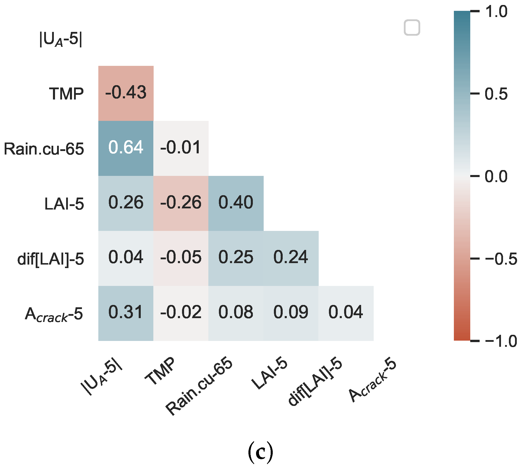
To avoid a complex model and over-fitting, uncorrelated features should be used as inputs. Therefore, the selected features are tested to examine if they are highly correlated or not. In Figure 9, the correlations between the selected features for all RF regressors are plotted. The features are not highly correlated and can therefore be used as candidate features to build the models for real-time assessment (Figure 9a) and short-term prediction (Figure 9b,c).
3.3.2. Real-Time Assessment
The RF model is built and trained based on the selected hyper-parameters and features. The feature importance values constitute the relative predictive power of the features and are shown in Table 4, where surface displacement () is seen to have the highest importance, 0.42. It is also shown in Section 3.2 that has a strong correlation with FoS. Cumulative rainfall during the last 65 days () has the second highest importance, with a feature importance of 0.22, and at the event day has a lower importance of 0.17. The feature importance of both vegetation growth over the past 15 days () and temperature () are low, 0.1 and 0.07 respectively. The displacement is the most direct proxy for the water effect within the dike, whereas the rainfall amount and amount of vegetation and temperature influence the water flux, therefore it is logical that they have a lower importance. The rate of vegetation growth is influenced by various climatic variables, and was seen previously [41] to have a different response at different times of the year, therefore it is reasonable for it to have the lowest importance.
Figure 10a,b show the predicted FoS versus the numerically calculated FoS for the test set and the evaluation set, respectively. The points in these two plots are colourised based on . The coefficient of correlation (R) between the predicted and calculated FoS in the test data set is 0.94 and RMSE = 0.05. It is clear that the model performs well on the unseen data (test set) that is within its training sample space (Figure 10a). However, when it comes to the evaluation set, the model performance deteriorates (Figure 10b); R = 0.31 and RMSE = 0.1. The latter value is considered a high error, since the range of calculated FoS in 2018 is from (almost) 0.8 to 1.4 (although both the R and RMSE are affected by the lower range of values). The variation of predicted and calculated FoS in 2018 is shown by the left-hand side y-axis and the dashed and dotted lines, and precipitation in the same period is shown by the right-hand side y-axis and starts in Figure 10c. The low performance of the RF on the evaluation set can be explained based on the latter figure; until further crack growth takes place, the predicted FoS is very close to the calculated FoS (before 22 July 2018) (R = 0.82; RMSE = 0.04). This is also reflected on Figure 10b by orange markers close to the diagonal line. Once cracks start growing after 22 July 2018, the predicted FoS deviates from the calculated FoS (red markers on Figure 10b). This is particularly clear on the day with the heaviest precipitation in September 2018 (see Figure 10c), which causes a large drop in calculated FoS. The (red) markers with the highest distance from the diagonal line correspond to rainy days after crack growth in July 2018. The RF cannot capture the response to the heavy rainfall which occurs in this period.
As explained in Section 3.1, when cracks grow, the calculated FoS is affected by and precipitation events (drop in FoS in August 2018). This shows that the model could not generalise (extrapolate) well on the training data before 2018. This is mainly attributed to the combination of rainfall intensity and unprecedented crack area. In order to investigate the effect of rainfall intensity on the same day that FoS is calculated, this parameter also included as a feature in building the next predictive model, RF. The feature importance of this model is similar to RF (Table 4), except that the added feature () has a very low impact on generally predicting FoS. Since the general results of these two models are almost the same, only the time series plot is shown in Figure 10d. The R value between the predicted and calculated FoS in the test data set is 0.96 and RMSE = 0.05 for RF, and in the evaluation data set, R = 0.32 and RMSE = 0.10. Using , the performance of the predictive models improves on days with heavy rainfall, e.g., in April and October 2018, where example results are emphasised with the blue box around them. In these periods, the predicted FoS using RF is responsive to significant rainfall events, where the predicted FoS drops, following the trends in the calculated results, which is significant for predicting unsafe situations.
In an attempt to improve RF performance, a new model (RF) is built using as a feature, along with other features. The feature importance is shown in Table 4. has the highest importance among the other features (0.47). has the second highest feature importance (0.25) and then it is followed by other features. The importance order of the observable features follows RF.
In Figure 11a,b, the predicted FoS from the testing and evaluation data set using the RF model is plotted against the calculated FoS in the corresponding data set, respectively. The R value between the predicted and calculated FoS in the test data set increased to 0.98 and the RMSE decreased to 0.03 (in respect to R = 0.96 and RMSE = 0.05 for RF). For the evaluation data set, R = 0.56 and the RMSE = 0.07, an improvement compared to the RF model performance over the evaluation data set (year 2018). According to the time series plot (Figure 11c), the overall performance of RF is improved compared to RF. Yet, the predicted values over-estimate the FoS after the crack expands on 22 July 2018, mostly due to the unprecedented low values, as explained before. In addition, the RF model has a significantly smaller response to the heavy rainfall events in August–September 2018 than observed. According to Table 4, has relatively low influence (feature importance = 0.11) on the FoS prediction. This causes a deviation in the predicted FoS for results after crack growth from the calculated FoS (red points in Figure 11c). However, when there is no heavy rainfall, e.g., in October 2018, RF performs well.
In total, when including the crack area as an input feature, in addition to those in the previous model, the model performance improves. It remains a difficult to observe feature, but warrants further investigation given its importance.
Results of this section show that the built RF models have low accuracy after the new trend takes place after growing cracks in summer 2018, because the RF model is not trained for the maximum crack area period. If an RF algorithm was trained over more diverse data of different cases, the RF models may have better performance.
3.3.3. Short Term Prediction
In this section, it is investigated whether an RF algorithm can give a short-term forecast for the dike safety. The used features are the same as before but for an earlier time. , and are selected 15 days before the event day. It is known that these have a lower correlation (see Figure 7), however this gives sufficient time to undertake further inspection and take action. To enhance RF performance, the meteorological data are used based on the event day, assuming that the climate data are predicted from different climate models which are quite reliable. The time of 15 days is selected as a period, where both the meteorological predictions may be reasonably accurate and which gives the dike managers enough time to take emergency inspection and remedial actions.
In Table 5, the feature importance for short-term prediction (15d) is shown. Like the previous analysis of RF, , 15 days before the event day (i.e., ), it has the maximum effect on FoS prediction, with the feature importance of 0.32. This is because, even with a 15-day lag, the correlation between displacement and FoS is relatively strong, −0.44 (Figure 7f). places in the second rank with the feature importance of 0.23, which does not have the 15 days lag, and the data up to the event day are used, considering the earlier assumption of meteorological data for the next 15 days. has the feature importance of 0.22. The feature importance of and have the least impact on the FoS prediction, like the previous analysis in Section 3.3.2, since these two features have a very low correlation with FoS (Figure 7e,f).
The results in Figure 12a, which are coloured by , show that for RF, R = 0.94 and RMSE = 0.06. The results for the evaluation data set (Figure 12b) show poor performance, i.e., R = 0.06 and RMSE = 0.14. As discussed before for RF, in the evaluation data set, after cracks grow, the red markers diverge from the diagonal line, showing the deviation of predicted FoS from calculated FoS after 22 July 2018. The markers that have the highest error in prediction correspond to heavy rainfall after crack expansion and cause reductions in calculated FoS, while RF cannot predict these values. In Figure 12b,c, the predicted FoS over 2018 is plotted against the calculated FoS in the independent data set. As before, it is seen that after the crack growth, the RF model cannot predict FoS accurately.
In an attempt to improve the results, two other analyses are tested. Firstly, as in the real-time assessment, the crack area is also considered as one of the features (RF); secondly, the period of the short term prediction decreased to 5 days (RF). For the former option, is selected from 15 days before the event day, and the other features remain as in the RF model.
As expected from previous analyses, has the highest impact on the RF performance (0.48); this is followed by with a feature importance of 0.17. Again, the order of the feature importance for the rest of the features is the same as in the previous analysis. has the relative importance of 0.13, then followed by with the relative importance of 0.11. The lowest relative importance is again for and .
The results of RF are shown in Figure 13. The performance of the RF model is increased compared to RF over both testing and evaluation data sets. Adding leads to a higher correlation between predicted and calculated FoS in the testing data set; R increased in order of 0.04 (R = 0.98) and RMSE is reduced by 0.02 (RMSE = 0.04) for the evaluation data set. Again, it can be inferred that after additional crack growth, the model cannot extrapolate FoS values for the heavy rainfall events, since the relative power of antecedent rainfall in predicting FoS is relatively low (feature importance = 0.13).
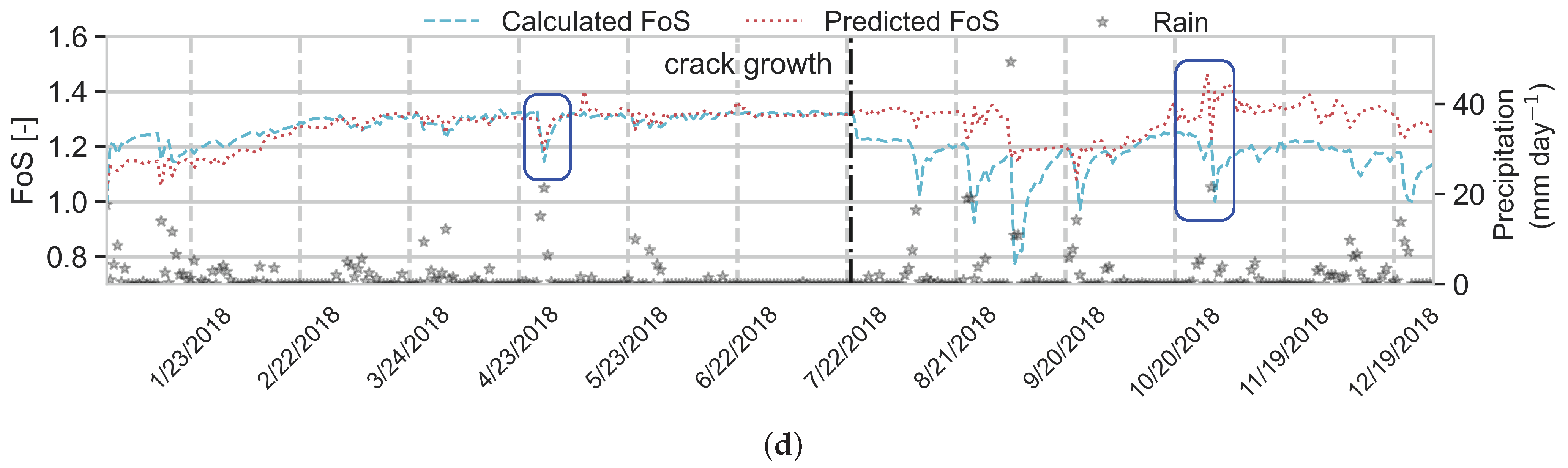
In another attempt to improve the short term prediction models, the lag is reduced to 5 days, which means that , and are selected from 5 days before the event day, while and are selected from the same day that FoS is predicted; is no longer considered. This period can be considered as sufficient to take emergency actions before a dike fails, e.g., evacuating a residential area.
The feature importance of RF model is shown in Table 5. Like the previous models, has the highest importance among other features, 0.36; this is between feature importance for in real-time assessment and for short-term prediction (15 days). The reason can be also concluded from Figure 7b: as the time lag increases, the correlation between FoS and decreases. The ranking order for other features for the RF is the same as short-term prediction with 15 days lag. However, the correlation between predicted and calculated FoS is increased in RF, R= 0.24 and RMSE= 0.12, compared to RF. As the lag decreases, the correlation between FoS and and increases, which leads to an increase in the power of the features in predicting the FoS. The time series plot for 5 days’ prediction is shown in Figure 14c (again like the previous analysis), the predicted FoS after crack growth in July 2018, which deviates from the calculated FoS. Although in RF, the deviation is less from the actual FoS compared to the results of RF, it still performed poorer than RF.
A summary of the build RF regressor ability to predict the FoS is given in Table 6, for the training data set, testing data set (which are randomly selected over the years 2009–2017) and the evaluation data set (year 2018). In both scenarios (real-time assessment and short-term prediction), if the crack area is used as one of the features, the model performance improves both in the testing data set and in the evaluation data set. In short-term prediction, when the time window is shortened from 15 days to 5 days, the RF model performance improves, since there is a higher correlation between the features that have the highest impact (, and ) and FoS at the shorter lag. Currently, it is not feasible to measure the crack area, but there are ongoing studies to simulate the crack volume, e.g., [57].
As shown in the results, using a RF regressor, the predicted values are never outside the training set values for the target variable (FoS). One of the RF regressor limitations is that it cannot extrapolate, because in the test set, it predicts an average of the values seen previously in the training. Therefore, the predicted FoS is bound to the minimum and maximum values of the build RF models seen in the training set. In the evaluation data set RF cannot, therefore, predict the minimum FoS values of the whole timeseries (2009–2018) that occurred after the training data set where the maximum occurs. To overcome this limitation, other algorithms can be used, e.g., deep learning, or combining predictors using stacking [47]. An alternative could be to undertake more numerical simulations of potential future scenarios to allow the RF regressor to ‘see’ potential future results. This research introduces that using a combination of EO data and predictive models can have a significant potential in the context of dike monitoring. This helps dike managers to be able to undertake real-time assessment and short-term predictions.
4. Conclusions
This proof-of-concept study investigates the potential use of observable data in predicting temporal changes in slope stability due to climatic forcing and includes the impact of vegetation and surface cracking. This study focused on making an ML-based surrogate for an FE model. The underlying assumption is that the FE model can emulate reality. Therefore, the validation against the ground truth data should be first reflected in the FE model evaluation. Using such an approach can provide experts with a monitoring tool where they can assess a significant length of dikes relatively easily. A random forest machine learning approach was adopted, with features used in the model (, surface displacement, cumulative rainfall and temperature) selected based on correlations with the FoS and that were potentially observable using satellite earth observation. This has advantages over using other features which require on-site investigation or the installation of permanent sensors. The results from the predictive model used in this study show that displacement has the highest feature importance for both cases of real-time assessment and short term prediction. It is recognised that, for other situations, slightly different features may be required. The approach resulted in an accurate prediction of the temporal FoS before new cracking events for the example dike. Over the ‘unseen’ data and after a crack expansion, the model performance is weak, as an RF model cannot extrapolate results and estimation is bound to the range of data over which the model has been trained. The results of this study show the potential use of EO data for real-time assessment and short-term prediction of an example dike condition. This method shows the potential of predictive models to support the assessment of a dike condition (stability), but not to replace more in-depth geotechnical site investigation and analysis. A single example dike was used as a case study to demonstrate the potential value of machine learning in general to circumvent the computational burden of modeling and taking an important first step towards large-scale monitoring of dike stability with EO data. It is suggested for future studies to include various real case studies to investigate the effectiveness of different ML algorithms for assessing a slope condition.
Author Contributions
Conceptualization, E.J. and F.S.T.; Formal analysis, E.J. and F.S.T.; Funding acquisition, P.J.V.; Investigation, E.J.; Methodology, E.J., F.S.T., S.C.S.-D. and P.J.V.; Project administration, P.J.V.; Supervision, F.S.T., S.C.S.-D. and P.J.V.; Validation, F.S.T., S.C.S.-D. and P.J.V.; Visualization, E.J.; Writing—original draft, E.J.; Writing—review & editing, F.S.T., S.C.S.-D. and P.J.V. All authors have read and agreed to the published version of the manuscript.
Funding
This research was funded by Netherlands Organisation for Scientific Research (NWO) grant number 13864.
Institutional Review Board Statement
Not applicable.
Informed Consent Statement
Not applicable.
Data Availability Statement
Not applicable.
Acknowledgments
This work is part of the research program Reliable Dikes with project number 13864, which is financed by the Netherlands Organisation for Scientific Research (NWO). The second author acknowledges the support of Deltares Strategic Research for his contribution to this study.
Conflicts of Interest
The authors declare that they have no conflict of interest.
References
- CIRIA; Ecology, F.M.; USACE. The International Levee Handbook; CIRIA: London, UK, 2013. [Google Scholar]
- De Vries, G. Monitoring Droogteonderzoek Veenkaden; Technical Report; Deltares: Delft, The Netherlands, 2012. [Google Scholar]
- Cundill, S.L. Investigation of Remote Sensing for Dike Inspection. Ph.D. Thesis, University of Twente, Twente, The Netherlands, 2014. [Google Scholar]
- Ozer, I. Understanding Levee Failures from Historical and Satellite Observations. Ph.D. Thesis, Delft University of Technology, Delft, The Netherlands, 2020. [Google Scholar] [CrossRef]
- Van Baars, S. The horizontal failure mechanism of the Wilnis peat dyke. Géotechnique 2005, 55, 319–323. [Google Scholar] [CrossRef]
- Pourghasemi, H.R.; Rahmati, O. Prediction of the landslide susceptibility: Which algorithm, which precision? Catena 2018, 162, 177–192. [Google Scholar] [CrossRef]
- Ada, M.; San, B.T. Comparison of machine-learning techniques for landslide susceptibility mapping using two-level random sampling (2LRS) in Alakir catchment area, Antalya, Turkey. Nat. Hazards 2018, 90, 237–263. [Google Scholar] [CrossRef]
- Baum, R.L.; Godt, J.W.; Savage, W.Z. Estimating the timing and location of shallow rainfall-induced landslides using a model for transient, unsaturated infiltration. J. Geophys. Res. Earth Surf. 2010, 115. [Google Scholar] [CrossRef]
- Conte, E.; Troncone, A. Analytical method for predicting the mobility of slow-moving landslides owing to groundwater fluctuations. J. Geotech. Geoenviron. Eng. 2011, 137, 777–784. [Google Scholar] [CrossRef]
- Conte, E.; Troncone, A. Stability analysis of infinite clayey slopes subjected to pore pressure changes. Géotechnique 2012, 62, 87–91. [Google Scholar] [CrossRef]
- Conte, E.; Donato, A.; Pugliese, L.; Troncone, A. Analysis of the Maierato landslide (Calabria, Southern Italy). Landslides 2018, 15, 1935–1950. [Google Scholar] [CrossRef]
- Yilmaz, I. Comparison of landslide susceptibility mapping methodologies for Koyulhisar, Turkey: Conditional probability, logistic regression, artificial neural networks, and support vector machine. Environ. Earth Sci. 2010, 61, 821–836. [Google Scholar] [CrossRef]
- Mokarram, M.; Zarei, A.R. Landslide Susceptibility Mapping Using Fuzzy-AHP. Geotech. Geol. Eng. 2018, 36, 3931–3943. [Google Scholar] [CrossRef]
- Raja, N.B.; Çiçek, I.; Türkoğlu, N.; Aydin, O.; Kawasaki, A. Landslide susceptibility mapping of the Sera River Basin using logistic regression model. Nat. Hazards 2017, 85, 1323–1346. [Google Scholar] [CrossRef] [Green Version]
- Chen, W.; Pourghasemi, H.R.; Kornejady, A.; Zhang, N. Landslide spatial modeling: Introducing new ensembles of ANN, MaxEnt, and SVM machine learning techniques. Geoderma 2017, 305, 314–327. [Google Scholar] [CrossRef]
- Youssef, A.M.; Pourghasemi, H.R.; Pourtaghi, Z.S.; Al-Katheeri, M.M. Landslide susceptibility mapping using random forest, boosted regression tree, classification and regression tree, and general linear models and comparison of their performance at Wadi Tayyah Basin, Asir Region, Saudi Arabia. Landslides 2016, 13, 839–856. [Google Scholar] [CrossRef]
- Steger, S.; Brenning, A.; Bell, R.; Petschko, H.; Glade, T. Exploring discrepancies between quantitative validation results and the geomorphic plausibility of statistical landslide susceptibility maps. Geomorphology 2016, 262, 8–23. [Google Scholar] [CrossRef]
- Reichenbach, P.; Rossi, M.; Malamud, B.D.; Mihir, M.; Guzzetti, F. A review of statistically-based landslide susceptibility models. Earth-Sci. Rev. 2018, 180, 60–91. [Google Scholar] [CrossRef]
- Pradhan, B. A comparative study on the predictive ability of the decision tree, support vector machine and neuro-fuzzy models in landslide susceptibility mapping using GIS. Comput. Geosci. 2013, 51, 350–365. [Google Scholar] [CrossRef]
- Pourghasemi, H.R.; Yansari, Z.T.; Panagos, P.; Pradhan, B. Analysis and evaluation of landslide susceptibility: A review on articles published during 2005–2016 (periods of 2005–2012 and 2013–2016). Arab. J. Geosci. 2018, 11, 193. [Google Scholar] [CrossRef]
- Goetz, J.; Brenning, A.; Petschko, H.; Leopold, P. Evaluating machine learning and statistical prediction techniques for landslide susceptibility modeling. Comput. Geosci. 2015, 81, 1–11. [Google Scholar] [CrossRef]
- Rossi, M.; Kirschbaum, D.; Luciani, S.; Mondini, A.C.; Guzzetti, F. TRMM satellite rainfall estimates for landslide early warning in Italy: Preliminary results. In Proceedings of the Remote Sensing of the Atmosphere, Clouds, and Precipitation IV, International Society for Optics and Photonics, Kyoto, Japan, 29–31 October 2012; Volume 8523, p. 85230D. [Google Scholar] [CrossRef]
- Kirschbaum, D.B.; Stanley, T.; Simmons, J. A dynamic landslide hazard assessment system for Central America and Hispaniola. Nat. Hazards Earth Syst. Sci. 2015, 15. [Google Scholar] [CrossRef] [Green Version]
- Hartke, S. Accounting for Satellite Precipitation Uncertainty: The Development of a Probabilistic Landslide Hazard Nowcasting System. Master’s Thesis, University of Wisconsin-Madison, Madison, WI, USA, 2019. [Google Scholar]
- Kirschbaum, D.; Stanley, T. Satellite-based assessment of rainfall-triggered landslide hazard for situational awareness. Earth’s Future 2018, 6, 505–523. [Google Scholar] [CrossRef]
- Jia, G.; Tang, Q.; Xu, X. Evaluating the performances of satellite-based rainfall data for global rainfall-induced landslide warnings. Landslides 2020, 17, 283–299. [Google Scholar] [CrossRef]
- Segoni, S.; Lagomarsino, D.; Fanti, R.; Moretti, S.; Casagli, N. Integration of rainfall thresholds and susceptibility maps in the Emilia Romagna (Italy) regional-scale landslide warning system. Landslides 2015, 12, 773–785. [Google Scholar] [CrossRef] [Green Version]
- Tien Bui, D.; Tuan, T.A.; Klempe, H.; Pradhan, B.; Revhaug, I. Spatial prediction models for shallow landslide hazards: A comparative assessment of the efficacy of support vector machines, artificial neural networks, kernel logistic regression, and logistic model tree. Landslides 2016, 13, 361–378. [Google Scholar] [CrossRef]
- Wei, X.; Zhang, L.; Yang, H.Q.; Zhang, L.; Yao, Y.P. Machine learning for pore-water pressure time-series prediction: Application of recurrent neural networks. Geosci. Front. 2020. [Google Scholar] [CrossRef]
- Chakraborty, A.; Goswami, D.D. Slope Stability Prediction using Artificial Neural Network (ANN). Int. J. Eng. Comput. Sci. 2017, 6. [Google Scholar] [CrossRef]
- Pei, H.; Zhang, S.; Borana, L.; Zhao, Y.; Yin, J. Slope stability analysis based on real-time displacement measurements. Measurement 2019, 131, 686–693. [Google Scholar] [CrossRef]
- Qi, C.; Tang, X. Slope stability prediction using integrated metaheuristic and machine learning approaches: A comparative study. Comput. Ind. Eng. 2018, 118, 112–122. [Google Scholar] [CrossRef]
- Lin, Y.; Zhou, K.; Li, J. Prediction of slope stability using four supervised learning methods. IEEE Access 2018, 6, 31169–31179. [Google Scholar] [CrossRef]
- Breiman, L. Random forests. Mach. Learn. 2001, 45, 5–32. [Google Scholar] [CrossRef] [Green Version]
- Hojat, A.; Arosio, D.; Ivanov, V.I.; Loke, M.H.; Longoni, L.; Papini, M.; Tresoldi, G.; Zanzi, L. Quantifying seasonal 3D effects for a permanent electrical resistivity tomography monitoring system along the embankment of an irrigation canal. Near Surf. Geophys. 2020, 18, 427–443. [Google Scholar] [CrossRef]
- Jamalinia, E.; Vardon, P.J.; Steele-Dunne, S.C. The effect of soil-vegetation-atmosphere interaction on slope stability: A numerical study. Environ. Geotech. 2019. Ahead of print. [Google Scholar] [CrossRef] [Green Version]
- Hanssen, R.F. Radar Interferometry: Data Interpretation and Error Analysis; Springer Science & Business Media: Berlin/Heidelberg, Germany, 2001; Volume 2. [Google Scholar] [CrossRef] [Green Version]
- Ferretti, A.; Prati, C.; Rocca, F. Permanent scatterers in SAR interferometry. IEEE Trans. Geosci. Remot. Sens. 2001, 39, 8–20. [Google Scholar] [CrossRef]
- ESA. User Guid, Sentinel-1. 2020. Available online: https://sentinel.esa.int/web/sentinel/user-guides/sentinel-1-sar (accessed on 18 December 2020).
- Carlà, T.; Intrieri, E.; Raspini, F.; Bardi, F.; Farina, P.; Ferretti, A.; Colombo, D.; Novali, F.; Casagli, N. Perspectives on the prediction of catastrophic slope failures from satellite InSAR. Sci. Rep. 2019, 9, 14137. [Google Scholar] [CrossRef] [Green Version]
- Jamalinia, E.; Vardon, P.J.; Steele-Dunne, S.C. The impact of evaporation induced cracks and precipitation on temporal slope stability. Comput. Geotech. 2020, 122, 103506. [Google Scholar] [CrossRef]
- Jamalinia, E.; Vardon, P.; Steele-Dunne, S. Use of displacement as a proxy for dike safety. Proc. IAHS 2020, 382, 481–485. [Google Scholar] [CrossRef] [Green Version]
- de Gast, T.; Hicks, M.A.; van den Eijnden, A.P.; Vardon, P.J. On the reliability assessment of a controlled dyke failure. Géotechnique 2020, 1–16. [Google Scholar] [CrossRef]
- Plaxis, B.V. Plaxis Reference Manual 2018; PLAXIS: Delft, Netherlands, 2018. [Google Scholar]
- Bouman, B.A.M.; Schapendonk, A.H.C.M.; Stol, W.; van Kraalingen, D.W.G. Description of LINGRA, a model approach to evaluate potential productivities of grasslands in different European climate regions. Quant. Approaches Syst. Anal. 1996, 7, 11–58. [Google Scholar]
- Jamalinia, E.; Tehrani, F.S.; Steele-Dunne, S.C.; Vardon, P.J. Predicting rainfall induced slope stability using Random Forest regression and synthetic data. Understanding and Reducing Landslide Disaster Risk. In Proceedings of the 5th World Landslide Forum, Kyoto, Japan, 2–6 November 2021; pp. 223–229. [Google Scholar] [CrossRef]
- Pedregosa, F.; Varoquaux, G.; Gramfort, A.; Michel, V.; Thirion, B.; Grisel, O.; Blondel, M.; Prettenhofer, P.; Weiss, R.; Dubourg, V.; et al. Scikit-learn: Machine Learning in Python. J. Mach. Learn. Res. 2011, 12, 2825–2830. [Google Scholar] [CrossRef]
- Breiman, L.; Friedman, J.; Stone, C.J.; Olshen, R.A. Classification and Regression Trees; CRC Press: Boca Raton, FL, USA, 1984. [Google Scholar]
- Verikas, A.; Vaiciukynas, E.; Gelzinis, A.; Parker, J.; Olsson, M.C. Electromyographic patterns during golf swing: Activation sequence profiling and prediction of shot effectiveness. Sensors 2016, 16, 592. [Google Scholar] [CrossRef] [Green Version]
- Zhou, J.; Li, E.; Wei, H.; Li, C.; Qiao, Q.; Armaghani, D.J. Random forests and cubist algorithms for predicting shear strengths of rockfill materials. Appl. Sci. 2019, 9, 1621. [Google Scholar] [CrossRef] [Green Version]
- Hastie, T.; Tibshirani, R.; Friedman, J. The Elements of Statistical Learning: Data Mining, Inference, and Prediction; Springer Science & Business Media: Berlin/Heidelberg, Germany, 2009. [Google Scholar] [CrossRef]
- Probst, P.; Wright, M.N.; Boulesteix, A.L. Hyperparameters and tuning strategies for random forest. Wiley Interdiscip. Rev. Data Min. Knowl. Discov. 2019, 9, e1301. [Google Scholar] [CrossRef] [Green Version]
- Stone, M. Cross-validatory choice and assessment of statistical predictions. J. R. Stat. Soc. Ser. Methodol. 1974, 36, 111–133. [Google Scholar] [CrossRef]
- Schapendonk, A.H.C.M.; Stol, W.; van Kraalingen, D.W.G.; Bouman, B.A.M. LINGRA, a sink/source model to simulate grassland productivity in Europe. Eur. J. Agron. 1998, 9, 87–100. [Google Scholar] [CrossRef]
- Wolf, J. Grassland Data from PASK Study & Testing of LINGRA; Technical Report, ASEMARS; Alterra: Denver, CO, USA, 2006. [Google Scholar]
- Entekhabi, D.; Yueh, S.; O’Neill, P.E.; Kellogg, K.H.; Allen, A.; Bindlish, R.; Brown, M.; Chan, S.; Colliander, A.; Crow, W.T.; et al. SMAP Handbook. Soil Moisture Active Passive: Mapping Soil Moisture and Freeze/Thaw from Space; JPL Publication: Pasadena, CA, USA, 2014. [Google Scholar]
- Li, J.; Zhang, L. Geometric parameters and REV of a crack network in soil. Comput. Geotech. 2010, 37, 466–475. [Google Scholar] [CrossRef]
Figure 1.
Flow chart of numerical modelling procedure [46].
Figure 1.
Flow chart of numerical modelling procedure [46].

Figure 2.
Flow chart of machine learning (ML) procedure.

Figure 3.
Basic structure of RF regressor: are features, n is the number of trees, l is the target value (after [49]).
Figure 3.
Basic structure of RF regressor: are features, n is the number of trees, l is the target value (after [49]).

Figure 4.
Example dike simulation geometry.

Figure 5.
Daily values of inputs for the crop model from 2009 to 2019 (a) Precipitation; (b) Average temperature; (c) Average wind speed; (d) Radiation.
Figure 5.
Daily values of inputs for the crop model from 2009 to 2019 (a) Precipitation; (b) Average temperature; (c) Average wind speed; (d) Radiation.

Figure 6.
Time series outputs from the coupled model for 10 years; (a) crack area percentage (); (b) Leaf Area Index (); (c) rate of change over 15 days (); (d) average soil moisture in the root zone (); (e) ground water level at point A (); (f) magnitude of total displacement at point A (); (g) Factor of Safety (FoS).

Figure 7.
Lag correlation between FoS and (a) root zone saturation (); (b) magnitude of total displacement (); (c) ground water level at point A (); (d) ; (e) rate of change over 15 days (); (f) temperature (); (g) crack area (), (h) rain; (i) cumulative rainfall during the last 65 days.
Figure 7.
Lag correlation between FoS and (a) root zone saturation (); (b) magnitude of total displacement (); (c) ground water level at point A (); (d) ; (e) rate of change over 15 days (); (f) temperature (); (g) crack area (), (h) rain; (i) cumulative rainfall during the last 65 days.

Figure 8.
Lag correlation between magnitude of surface displacement at points A and B.

Figure 9.
Correlation between features for (a) real-time assessment, (b,c) short-term prediction RF models with 15 days and 5 days lag, respectively.
Figure 9.
Correlation between features for (a) real-time assessment, (b,c) short-term prediction RF models with 15 days and 5 days lag, respectively.


Figure 10.
RF model performance, over (a) testing data set and (b) evaluation data set, and (c) time series of calculated and predicted FoS in the evaluation data set; (d) time series of calculated and predicted FoS in the evaluation data set using RF.
Figure 10.
RF model performance, over (a) testing data set and (b) evaluation data set, and (c) time series of calculated and predicted FoS in the evaluation data set; (d) time series of calculated and predicted FoS in the evaluation data set using RF.


Figure 11.
RF model performance, over (a) the testing data set and (b) the evaluation data set; and (c) time series of predicted and calculated FoS in the evaluation data set (year 2018).
Figure 11.
RF model performance, over (a) the testing data set and (b) the evaluation data set; and (c) time series of predicted and calculated FoS in the evaluation data set (year 2018).

Figure 12.
RF model performance, over (a) the testing data set and (b) the evaluation data set, and (c) time series of predicted and calculated FoS in the evaluation data set (year 2018).
Figure 12.
RF model performance, over (a) the testing data set and (b) the evaluation data set, and (c) time series of predicted and calculated FoS in the evaluation data set (year 2018).

Figure 13.
RF model performance, over (a) the testing data set and (b) the independent data set, and (c) time series of predicted and calculated FoS in the evaluation data set (year 2018).
Figure 13.
RF model performance, over (a) the testing data set and (b) the independent data set, and (c) time series of predicted and calculated FoS in the evaluation data set (year 2018).

Figure 14.
RF model performance, over (a) the testing data set and (b) the independent data set, and (c) time series of predicted and calculated FoS in the independent data set (year 2018).
Figure 14.
RF model performance, over (a) the testing data set and (b) the independent data set, and (c) time series of predicted and calculated FoS in the independent data set (year 2018).


Table 1.
Input parameters for non-cracked soil in the integrated model.
| Model Component | Parameters | Value | ||
|---|---|---|---|---|
| Crop sub-model | Soil | 0.29 (cmwater cmsoil) | ||
| 0.12 (cmwater cmsoil) | ||||
| 0.005 (cmwater cmsoil) | ||||
| 50 (mm day) | ||||
| Vegetation | 0.025 (m g) | |||
| 0.8 (m leaf mground) | ||||
| 4 (m leaf m ground) | ||||
| Root zone | Dike body | |||
| Geotechnical sub-model | Constitutive model | Saturated unit weight () | 20 (kN m) | 12 (kN m) |
| Intact friction angle () | 23 | 23 | ||
| Minimum friction angle () | 4.5 | - | ||
| Intact cohesion () | 2 (kPa) | 2 (kPa) | ||
| Minimum cohesion () | 0.6 (kPa) | - | ||
| Dilatancy angle () | 0 | 0 | ||
| Young’s modulus (E) | 10 (MPa) | 20 (MPa) | ||
| Poisson’s ratio () | 0.3 | 0.2 | ||
| Initial void ratio () | 0.67 | 1.2 | ||
| Hydraulic model | Permeability () | 0.14 (m day) | 0.03 (m day) | |
| Scale parameter | 1.47 (m) | 1.38 (m) | ||
| Fitting parameter n | 1.97 | 1.32 | ||
| Fitting parameter m | 0.87 | −1.24 | ||
Table 2.
List of candidate values for hyper-parameters for all RF models.
| Parameter | Tested Value |
|---|---|
| n-estimator | [10, 50, 100, 200, 300, 500, 700, 1000, 1500, 2000] |
| max tree-depth | [10, 30, 50, 70, 100, 150, 200] |
| min-samples-split | [2, 3, 4, 5, 8, 10] |
| min-samples-leaf | [1, 2, 3, 4, 5] |
Table 3.
Tuned hyper-parameters for constructed RF models.
| RF Model | n-Estimator | Max Tree-Depth | Min-Samples-Split | Min-Samples-Leaf |
|---|---|---|---|---|
| RF | 700 | 200 | 2 | 1 |
| RF | 700 | 70 | 2 | 1 |
| RF | 2000 | 200 | 2 | 1 |
| RF | 700 | 30 | 2 | 1 |
| RF | 1500 | 30 | 2 | 1 |
| RF | 1000 | 100 | 2 | 1 |
Table 4.
Feature importance for real-time assessment RF models.
| RF Model | |||||||
|---|---|---|---|---|---|---|---|
| RF | - | 0.42 | 0.22 | 0.17 | 0.1 | 0.07 | - |
| RF | - | 0.40 | 0.21 | 0.16 | 0.09 | 0.06 | 0.06 |
| RF | 0.47 | 0.25 | 0.11 | 0.07 | 0.04 | 0.03 | - |
Table 5.
Feature importance for short-term prediction RF models.
| Features | -15/5d | -15/5d | -65 | -15/5d | -15/5d | |
|---|---|---|---|---|---|---|
| RF | - | 0.32 | 0.23 | 0.22 | 0.10 | 0.08 |
| RF | 0.48 | 0.17 | 0.13 | 0.11 | 0.05 | 0.05 |
| RF | - | 0.36 | 0.23 | 0.19 | 0.12 | 0.08 |
Table 6.
Summary of RF models performance on all data sets.
| Scenarios | Training | Testing | Evaluation | ||||
|---|---|---|---|---|---|---|---|
| R | RMSE | R | RMSE | R | RMSE | ||
| Real-time assessment | observable features (5 features) | 0.99 | 0.01 | 0.96 | 0.05 | 0.31 | 0.1 |
| observable features(6 features) | 0.99 | 0.01 | 0.98 | 0.05 | 0.32 | 0.1 | |
| observable and crack area as features | 1 | 0.01 | 0.98 | 0.03 | 0.56 | 0.07 | |
| Short-term prediction | observable features (15 days lag) | 0.99 | 0.01 | 0.94 | 0.06 | 0.06 | 0.14 |
| observable and crack area as features (15 days lag) | 0.99 | 0.01 | 0.98 | 0.04 | 0.44 | 0.08 | |
| observable features (5 days lag) | 0.99 | 0.01 | 0.96 | 0.05 | 0.24 | 0.12 | |
Publisher’s Note: MDPI stays neutral with regard to jurisdictional claims in published maps and institutional affiliations. |
© 2021 by the authors. Licensee MDPI, Basel, Switzerland. This article is an open access article distributed under the terms and conditions of the Creative Commons Attribution (CC BY) license (http://creativecommons.org/licenses/by/4.0/).
Share and Cite
MDPI and ACS Style
Jamalinia, E.; Tehrani, F.S.; Steele-Dunne, S.C.; Vardon, P.J. A Data-Driven Surrogate Approach for the Temporal Stability Forecasting of Vegetation Covered Dikes. Water 2021, 13, 107. https://doi.org/10.3390/w13010107
AMA Style
Jamalinia E, Tehrani FS, Steele-Dunne SC, Vardon PJ. A Data-Driven Surrogate Approach for the Temporal Stability Forecasting of Vegetation Covered Dikes. Water. 2021; 13(1):107. https://doi.org/10.3390/w13010107
Chicago/Turabian StyleJamalinia, Elahe, Faraz S. Tehrani, Susan C. Steele-Dunne, and Philip J. Vardon. 2021. "A Data-Driven Surrogate Approach for the Temporal Stability Forecasting of Vegetation Covered Dikes" Water 13, no. 1: 107. https://doi.org/10.3390/w13010107
Note that from the first issue of 2016, this journal uses article numbers instead of page numbers. See further details here.