Multi-Objective Optimization for Analysis of Changing Trade-Offs in the Nepalese Water–Energy–Food Nexus with Hydropower Development

Abstract

While the water–energy–food nexus approach is becoming increasingly important for more efficient resource utilization and economic development, limited quantitative tools are available to incorporate the approach in decision-making. We propose a spatially explicit framework that couples two well-established water and power system models to develop a decision support tool combining multiple nexus objectives in a linear objective function. To demonstrate our framework, we compare eight Nepalese power development scenarios based on five nexus objectives: minimization of power deficit, maintenance of water availability for irrigation to support food self-sufficiency, reduction in flood risk, maintenance of environmental flows, and maximization of power export. The deterministic multi-objective optimization model is spatially resolved to enable realistic representation of the nexus linkages and accounts for power transmission constraints using an optimal power flow approach. Basin inflows, hydropower plant specifications, reservoir characteristics, reservoir rules, irrigation water demand, environmental flow requirements, power demand, and transmission line properties are provided as model inputs. The trade-offs and synergies among these objectives were visualized for each scenario under multiple environmental flow and power demand requirements. Spatially disaggregated model outputs allowed for the comparison of scenarios not only based on fulfillment of nexus objectives but also scenario compatibility with existing infrastructure, supporting the identification of projects that enhance overall system efficiency. Though the model is applied to the Nepalese nexus from a power development perspective here, it can be extended and adapted for other problems.

1. Introduction

A lack of cross-sector coordination is hampering efficient resource utilization in many developing countries like Nepal [1,2,3,4]. Despite the abundance of water resources in Nepal, poor governance and inequitable access can worsen water scarcity if the current pressures of export-oriented hydropower development persist [5]. In such a context, the water–energy–food nexus approach can help us understand cross-sector trade-offs and identify coordinated development pathways that synchronize sectorial benefits [1,2,6,7]. The inextricable linkages arising from shared and interdependent resource usage across the water, energy, food, environment, and other sectors create a complex nexus [8,9]. The nexus approach refers to a new paradigm for environmental governance whereby these interdependencies are systematically analyzed in a holistic framework to identify management policies that can integrate diverse cross-sectorial goals [1,2]. It promotes sustainable economies that maximize overall resource use efficiency and productivity across sectors by capitalizing on existing synergies across the water, energy and food sectors [3,9]. For the specific context of Nepalese hydropower development, Gyawali [10] demonstrate that the nexus approach can fuel a conscious development of multi- instead of single-purpose water infrastructures.

Even though the nexus approach has been extensively discussed at a conceptual level, quantitative methods to include the approach in decision-making are limited [1,3,11]. Bizikova et al. [11] review the principal qualitative nexus frameworks, while Flammini et al. [12] summarize quantitative frameworks in their review. Representing interdisciplinary systems in a quantitative nexus framework that is easy to adopt, understand, and apply across various contexts and spatial scales is a challenge [3]. Such a framework needs to embody systems thinking, accommodate varying spatial scales for different resource uses, and find innovative ways to integrate existing models that tend to focus on the use of a single resource [3,13]. For instance, Howells et al. [14] present a nexus modeling framework that integrates Water Evaluation and Planning (WEAP), Long-range Energy Alternatives Planning (LEAP), and Agro-ecological Zoning (AZE) models by linking their inputs and outputs to analyze resource allocation under various climate change scenarios. Giampietro et al. [15] extend an accounting-based model initially developed to analyze metabolic patterns of energy to implement the nexus approach. Similarly, multi-objective optimization, traditionally used for hydropower scheduling, is being adopted as a quantitative tool for decision-making in the nexus [13,16,17].

Multi-objective optimization has long been used in a wide array of water resources planning and management problems to evaluate trade-offs between conflicting objectives in the form of Pareto or trade-off fronts [17,18,19,20,21,22]. Pareto fronts represent the set of all possible Pareto-optimal solutions to a multi-objective problem. Each Pareto-optimal solution refers to a state of resource allocation where improvement in one objective cannot be achieved without decreasing the performance in another [20,23]. By visualizing the trade-offs between different objectives, Pareto fronts can reveal where greater efficiency in resource allocation can be attained and help policy makers understand the change in trade-offs presented by new policies [17,24]. The ability to account for diverse aspects of a problem using different objective functions makes multi-objective optimization well suited for representing the complexities of the nexus.

Weighting and constraining methods were the first techniques developed for formulating multi-objective problems by parametrically varying linear combination of weights or constraints placed on the multiple objectives [19,20,25]. These belong to the class of a posteriori decision support methods, where the full trade-off front is generated with no prior articulation of preferences [25]. Mathematical programming is used to iteratively solve each set of weights or constraints to generate the set of Pareto optimal points [19,26]. The initial application of multi-objective optimization in infrastructure planning eventually shifted towards improvement of existing operations as investments in new infrastructure declined [21,27,28]. As a consequence, more realistic non-linear simulation-based methods have been used extensively to inform efficient reservoir operation [21] (for review of examples see: [25,29,30]). While evolutionary algorithms have been adopted as preferred solvers for such non-linear multi-objective problems [25,29,31,32], infrastructure planning problems spanning multiple years continue to use linear programming (LP) [33,34,35,36] as it can efficiently accommodate high dimensionality and does not require fine tuning like evolutionary algorithms [29,37].

The Nepalese government’s plans to increase hydropower capacity from 790 MW up to 37,628 MW by 2030 provide an appropriate context to demonstrate the potential of multi-objective optimization to formally assess the nexus linkages to inform infrastructure development decisions. The nexus approach can be seen as a systematic way to adopt the recommendations of the World Commission on Dams to expand traditional ‘silo’ approaches in decision-making [38]. The holistic principles of the nexus allow for a more comprehensive evaluation of the benefits, impacts and risks of proposed projects across sectors and ensure sustainability and equity in development [1,2]. As Bazilian et al. [3] point out, the relevance of the nexus approach in hydropower decision-making is apparent but its adoption has been limited. Only a few studies like [39,40] have explored the nexus linkages in hydropower quantitatively. Hydropower does not significantly change available water quantity but alters the pattern in river flows affecting crop production and biodiversity downstream [3,38,41,42].

Ensuring water availability for hydropower generation and food production is a compounding nexus challenge under increasing water stresses and food scarcity in South Asia [43,44]. Based on the analysis of the South Asian nexus from the perspective of food security, Rasul [6] proposed a nexus framework where quantification of interactions across the water, energy, and food sectors, including inherent tradeoffs, is a key step. Rasul [6,44] emphasize the need for an integrated modeling study to understand the spatial dimensions of the interdependencies because the South Asian nexus is characterized by heavy reliance of the downstream communities on services provided by the upstream Himalayas. While the seasonal pattern in basin inflows is often well understood, the variety of water users across a basin can make it difficult to predict local water availability for specific purposes. Food security assessments, in particular, need to note when and where water availability is insufficient to support desired crop production to identify vulnerable zones [45]. A spatially explicit multi-objective optimization can address these issues by incorporating various water users in the water–energy–food nexus in a single framework and help streamline plans to strengthen water, energy, and food security.

Using the context of the Nepalese hydropower development, this study demonstrates a novel coupling of a linear water resources model [20] and a direct current (DC) load flow based optimal power flow (OFP) model [46] with fine spatial discretization to realistically model tradeoffs and synergies in the water–energy–food nexus. A flow path based network representation of water systems presented by Cheng et al. [47] is applied to represent upstream and downstream linkages, while the OPF model captures restrictions in power transmission. Physical constraints in the power and water systems have been modeled in detail as they can result in higher deficits, inequity in resource utilization, and even altered inter-dependencies in the nexus. Disaggregation is also key for identifying spatial variation in irrigation water availability and resulting self-sufficiency in food production throughout the basin. Specifically, an LP-based multi-objective optimization model is applied to the Nepalese water-energy-food nexus to analyze trade-offs between five cross-sector challenges—power deficit, irrigation water deficit, flood risk, environmental impact, and power export—under eight hydropower development scenarios. Multi-objective optimization is presented as a quantitative approach to understand the impact of infrastructure development on overall water management and help the divided sectors in the government realize that development pathways could fulfill multiple objectives concurrently [1,2]. This study contributes a disaggregated, linear, multi-objective optimization model that represents water and power systems explicitly using two overlapping networks to realistically model the spatiotemporal dependencies in the water–energy–food nexus.

2. Methods

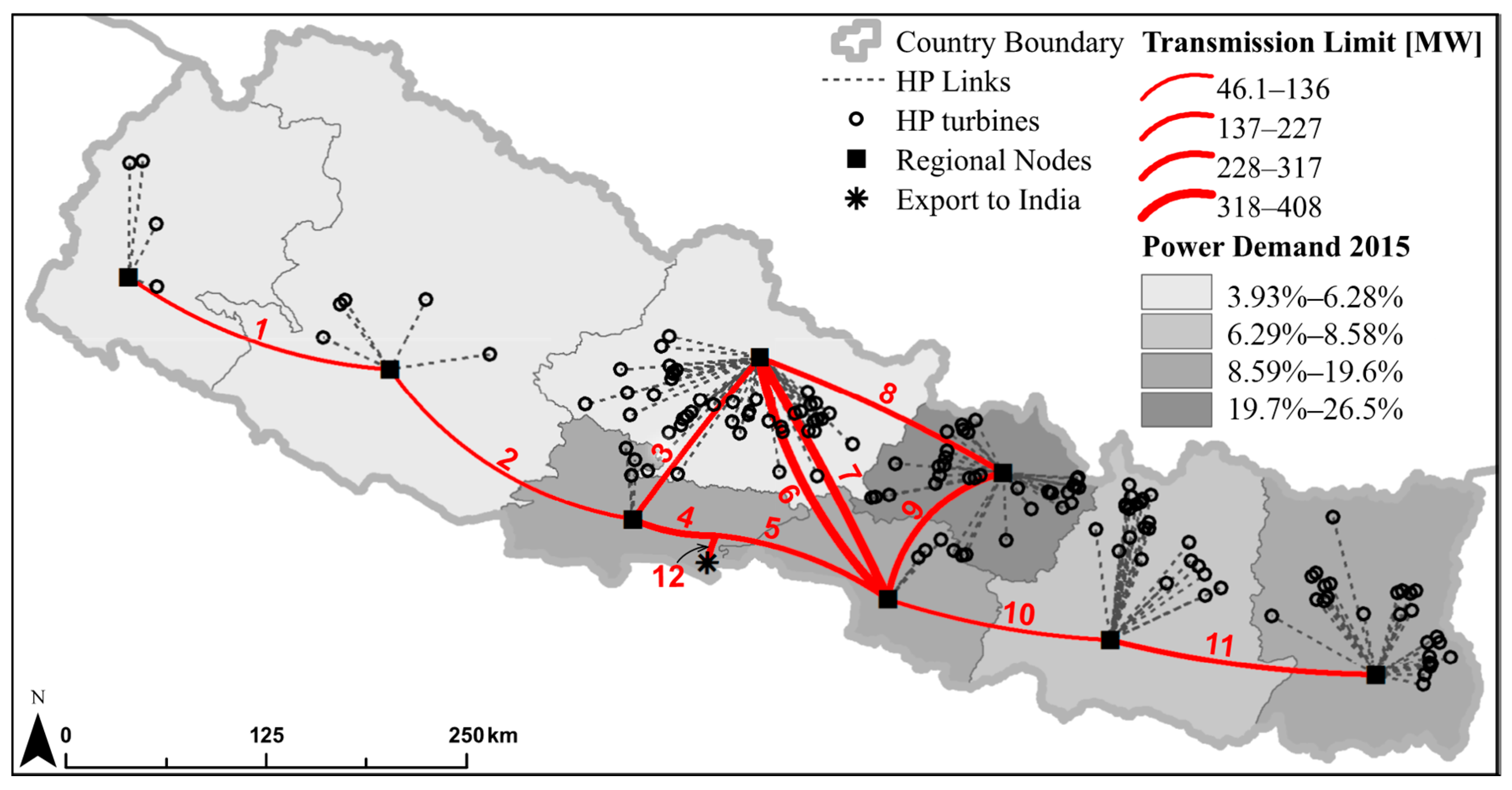
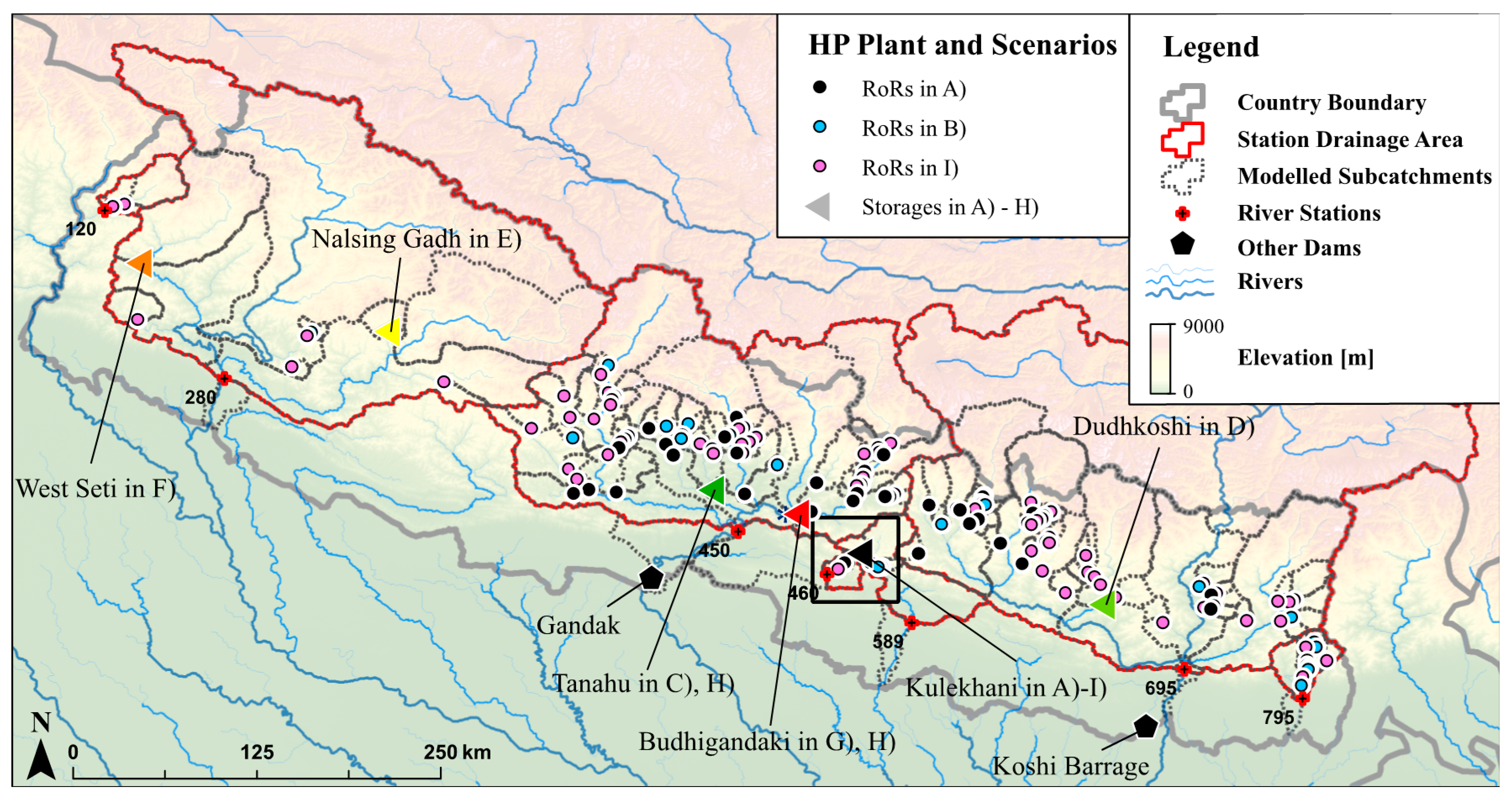
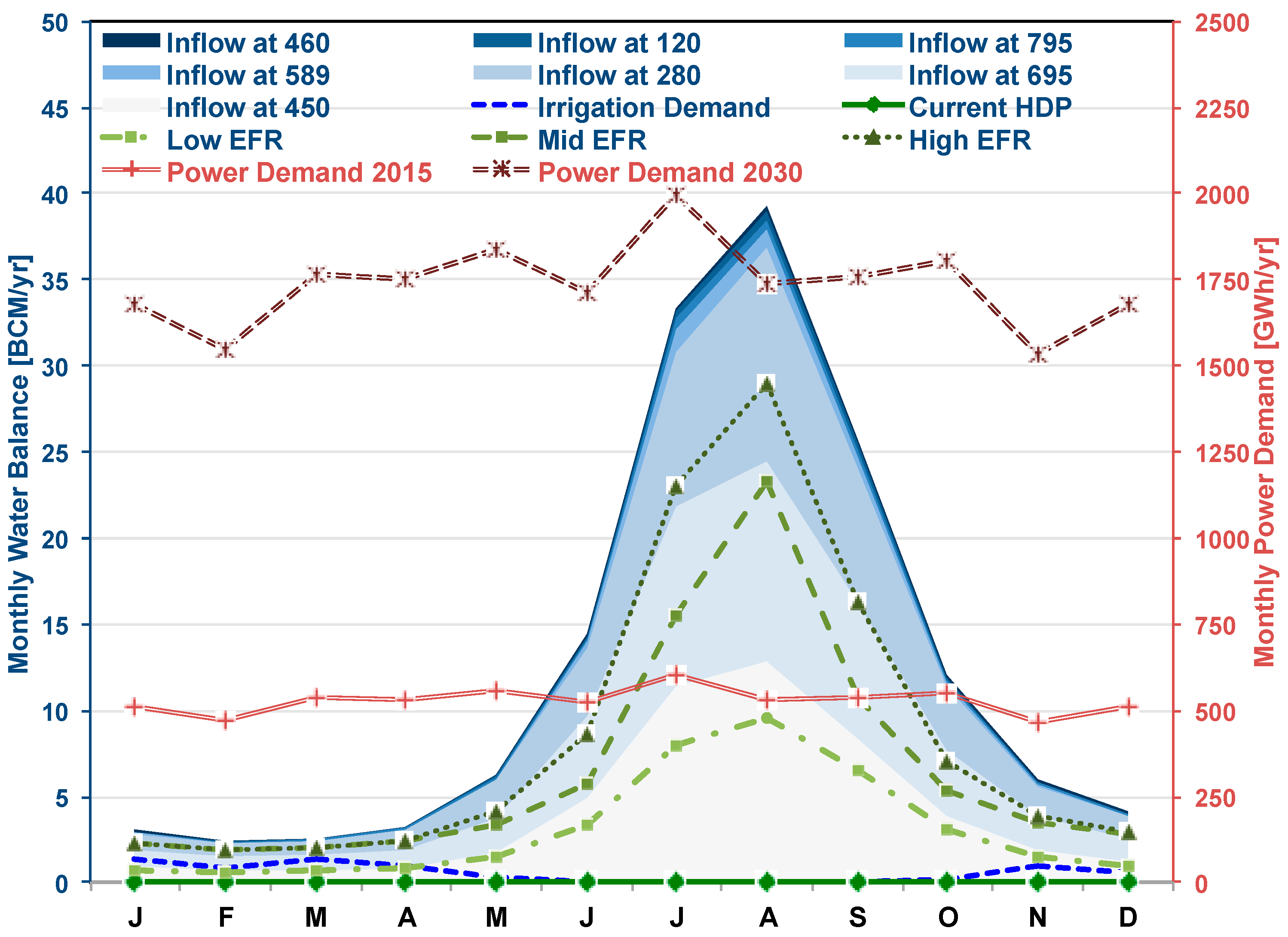
2.1. The Case of Nepal

Over 6000 rivers make up the 10 river basins in Nepal and are a source of both hope and fear. These snow- and rain-fed rivers provide water for irrigation and hydropower production, while fueling fear of floods that have caused an average of 269 deaths annually [48]. Along with the river systems in Nepal, Figure 1 shows three existing dams—at the Koshi barrage to prevent flooding, at Kulekhani to generate hydropower, and at Gandak to divert water for both hydropower and irrigation. Besides these, 39 run-of-river plants (RoR) and a few public irrigation schemes exist. This relatively unaltered state of the river basins will change under the new irrigation and power expansion plans proposed in the Hydropower Development Policy (HDP) [49] and National Water Plan [50]; consequently, patterns in water availability and flood risks may vary.

Table 1. Average annual demand and supply thresholds within modeled areas input to model.

Parameter		Quantity	Unit	Adapted from
Inflow for 1995–2008		152	109 m3/year	[53]
Environmental Flow Requirement (EFR)	HDP	0.673	109 m3/year	[55]
	Low	37.5	109 m3/year
	Mid	79.1	109 m3/year
	High	104	109 m3/year
Irrigation Demand		7.03	109 m3/year	[45]
Power Demand	2015	6335	GWh/year	[56,57]
	2030	20,811.80	GWh/year	[56,58]

summarizes the annual averages for water and power demand and supply in Nepal while Figure 2 presents their monthly distributions. Inflow is evaluated based on 14-year historical (1995–2008) daily inflow series provided by Rijal [53], from seven downstream river stations in each modeled basin, indicated in Figure 1. The high seasonality in inflow is due to the precipitation pattern, where 80 percent of total rainfall falls in the monsoon period (June–September) [54]. Because of a lack of older data and limited alteration of natural hydrology, these inflows are considered representative of the natural flow.

Agriculture is the most significant water user, accounting for 95.9% of all annual withdrawal [59]. Despite the dominance of rain-fed agriculture, irrigation demands are high due to water-intensive cereal crops—paddy, maize, and wheat, which are staples in the region. Maize is largely a rain-fed crop, whereas paddy and wheat are both rain-fed and irrigated depending on the location and season [54]. Irrigation is currently considered important only in the dry months to support winter crops [44,54]. While the cropping areas for major crops have remained relatively stable in the last decade, total crop production has increased due to expansion in irrigation, use of improved seeds, and higher cropping intensities [60]. However, food deficit is a reality in many districts in the mountains where agricultural conditions are harsh and limited infrastructure exists to support local food production [54]. Fang et al. [61] point out that western districts are most vulnerable to food scarcity because these areas have high poverty and scarce road networks limiting external food supply. Both cropping intensity and year-round irrigation facilities need to be expanded to ensure food self-sufficiency in Nepal under current population growth and climate change [50,62]. Rasul [6] highlights that current policies and subsidies targeting an increase of crop production in the region have led to significantly higher demands for water and energy. An assessment of water availability for irrigation is necessary to ensure food security in the long run and provide a basis for establishing sustainable policies.

However, no record of actual irrigation water withdrawal is available. Biemans et al.’s [43] is the only study providing spatially and temporally explicit estimates for irrigation water demand for South Asia based on a Lund-Potsdam-Jena managed Land (LpJmL) global hydrology and vegetation model. However, Biemans et al. ’s [43] estimate for the gross irrigation water demand of 2.34 × 10⁹ m³ for Nepal, assuming an irrigation efficiency of 37.5%, is significantly lower than that reported by other studies [62,63,64]. Gross irrigation water demand represents the sum of water required to fulfill evapotranspiration (crop transpiration and soil evaporation) requirements over the crop period and losses in conveyance and application. Portion of applied gross irrigation water that can be covered as part of return flows have not been considered here due to lack of prior estimates. Biemans et al. [43] suggest that their disaggregated model and their assumptions may produce lower estimates than predicted by older models that tend to be lumped and do not account for multiple cropping and monsoon dependent crop start dates. The Food and Agriculture Organization (FAO) [63] reports gross irrigation water demands of 9.32 × 10⁹ m³, which can be considered the best estimate for Nepal. The study [63] used the FAO crop coefficient method with a higher irrigation efficiency of 58%. In contrast to both studies, the Nepalese government reports an irrigation efficiency of 30% [50].

Despite the low estimates, Biemans et al. [43] provide the only available estimate of seasonal variation in irrigation demand. Therefore, a closer evaluation of Nepal-specific assumptions and a comparison of MICRA2000 land use data derived by Biemans et al. [43] and data published by the Nepalese government [60] was undertaken in a prior study [55]. Consequently, Biemans et al.’s [43] irrigation water demand estimates, including potentially recoverable return flows, were scaled up by a factor of 4 to be used as irrigation demand in this study. The irrigation water demand, shown in Figure 2, is out of phase with inflow due to the double and triple cropping practices common in the region. As agriculture is the most significant water user, the relatively low domestic and industrial water withdrawals are ignored in this study.

The existing power system in Nepal comprises of a single Integrated National Power System (INPS) grid; 73% of power supply is by HP plants [56]. Over 39 RoRs and the Kulekhani storage plant provide year-round energy, while 100 KW solar farms and a few seasonal plants like Gandak provide supplementary power [56]. The use of solar energy at household level is being encouraged [65], while fuel-based power plants are being phased out [56]. Monthly power demand is relatively stable. Figure 2 shows the demand pattern based on hourly demand for peak days of the month in 2013/2014 (provided by Shrestha [57]). Domestic consumers account for nearly 45% of the national power consumption while industries account for 36% and only 2% for water supply and irrigation [56]. Of the total demand recorded in the INPS grid in 2014/2015, 21% was not met. To fulfill the supply gap, the government imports power from India [56] and regularly cuts off power. Load shedding of as much as 14 h per day was imposed during the low flow season in 2016 [66]. The existing HP capacity (790 MW as of 2015) is not able to meet the annual demand and suffers irregular supply due to the dominance of RoRs. Long-term government plans are thus focused on building storage based HP plants to support urbanization, rural electrification, expansion of irrigation systems, modernization of agriculture and industrialization [67]. Revenue generation from power export, initially to India and then other South Asian countries based on existing regional agreements, is another motivation for the focus on HP development [67,68]. These multidimensional motivations for hydropower development in Nepal require a holistic nexus-based assessment of development scenarios for well-informed decision-making.

Figure 1 presents 141 HP plants in various stages of development (as indicated by their licensing status [52]), included in this study, while

Table 2. Power development scenarios and relevant features of storage plants analyzed in this study. Locations of all plants are indicated in Figure 1.

HP Development Scenarios		Added Capacity (MW)	Reservoir Capacity (MCM)	Head (m)	Discharge (m3/s)	Source
A)	Existing 39 RoRs + Kulekhani *	692	63.3	550	12.1	[72]
B)	A + 21 RoRs completed in 2016	203	-	multiple	multiple	[69]
C)	B + Tanahu	127	295.1	112.5	127	[73]
D)	B + Dudhkoshi	300	687.4	249.3	136	[70]
E)	B + Nalsing Gadh	410	419.6	635.5	75	[74]
F)	B + West Seti	750	1483	258	327	[75]
G)	B + Budhigandaki	1200	4467	200	672	[76]
H)	B + Tanahu + Budhigandaki	1327	See scenarios C and I
I)	B + 75 under-construction RoRs	1964	-	multiple	multiple	[52]

Note: * Reported volume, head, and discharges are for the existing Kulekhani reservoir.

summarizes the features of storage plants included in the nine modeled scenarios. Excluding some small and seasonal HP plants, 39 currently operational RoRs and the storage plant at Kulekhani are defined as existing scenario A). Scenario B) represents the existing 40 plants, supplemented by 21 RoRs that will finish construction in 2016 [69], while at least 75 other RoRs currently listed as under construction are added in I). Of the many candidates in discussion [70], five storage-based hydropower plants have been identified as most likely. These storage plants added to the base scenario B) are considered in scenarios C)–G). Additionally, scenario H), with two storage plants—Tanahu and Budhigandaki—is also considered. Other plants in the planning stages have been excluded. Besides power production, power transmission is also being expanded, but transmission expansion is not considered here as new plants are being developed faster than transmission lines [68,71].

Ongoing power development plans also pose a threat to the 118 ecosystems in the protected areas that cover 23 percent of the country [54,77]. While reasonable estimates for human demands are available, the needs of the environment, quantified here in terms of Environmental Flow Requirement (EFR), are not well established for Nepal. The HDP [49] arbitrarily stipulates a release requirement of 10% of long-term minimum monthly flow or minimum flow established in the environmental impact assessments, whichever is lower. However, such a requirement is too low when compared to well-established environmental flow benchmarks [78] and fails to consider flow variability [77,79].

Many developing countries like Nepal lack good baseline data and resources to successfully use rigorous eco-hydrological EFR assessment methods [80]. In the absence of clear ecological river management objectives, Acreman and Dunbar [79] and Dyson et al. [81] suggest scenario-based EFR setting where the impacts of an ensemble of EFRs are modeled to provide a basis for discussion between water managers and stakeholders. For scoping and basin-scale planning studies, as proposed here, simple hydrological methods are recommended [79,81]. Therefore, three hydrological environmental flow assessment methods, the modified Tennant [82], the modified Range Variability Approach (RVA) [83], and the shifted Flow Duration Curve method [84], were used to establish an ensemble of EFRs at the seven river stations prior to this study [55]. In addition to the HDP requirements, three EFRs are chosen from that ensemble to represent low, middle, and high EFR levels in this study.

Studies on the impacts of climate change suggest that temperatures are rising, resulting in increased glacier melt contribution to streamflow in the short run [64,85,86,87]. As de-glaciation is completed, streamflow is expected to decline; however, no generalizable trend in streamflow across the major basins has been established. An assessment of climate change impacts on Nepalese hydropower based on climate projections for 2040–2059 found that existing power plants appear robust, with a reduction in production seen only for RoR plants based on rain-fed rivers at lower elevations [88]. Climate change is not considered a dominant issue in the Nepalese nexus in the short to medium term. The assessment of climate change impacts is therefore left to future design studies for selected projects.

Analyzing the organic evolution of the usage of the existing Kulekhani reservoir over time, Gyawali [10] found that even though Kulekhani was strictly developed and operated as a single-purpose hydropower production reservoir at a government level, today it is actively supporting fishing, dry season irrigation downstream, drinking water supply, and tourism at a local level. Had initial plans for Kulekhani considered this potential multi-purpose usage, its benefits across different sectors could have been further maximized. Ongoing power development plans should learn from the case of Kulekhani and explore upstream–downstream linkages in the water–energy–food nexus from each proposed hydropower plants prior to decision-making. A quantitative assessment of trade-offs that exist in water, energy, food, and environmental management in Nepal can both aid the mainstreaming of the nexus approach in decision-making and encourage resource-efficient infrastructure development.

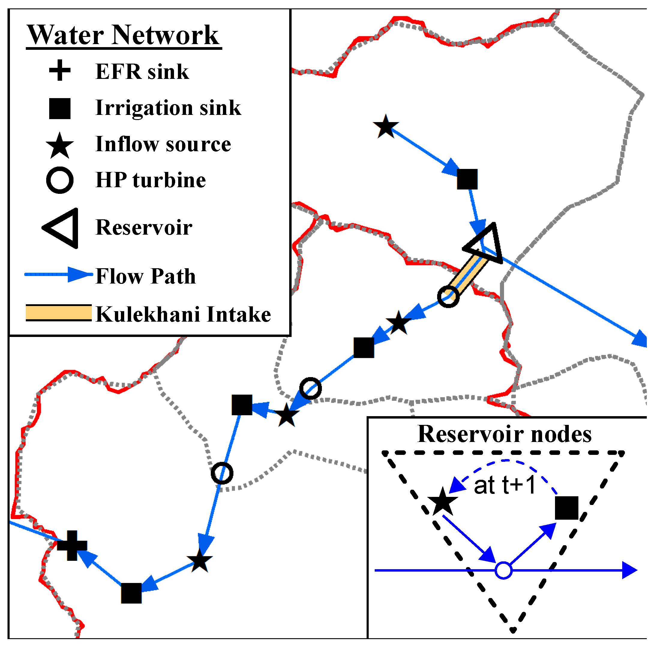
2.2. Representation of Water and Power Flows

Cheng et al. [47] provide a generalized methodology to represent water distribution networks in terms of flow paths indicating all possible water delivery routes from each source node to the associated demand nodes. Such a flow path representation allows for automated setup of the model constraints, as described in Dhaubanjar [55]. Similar flow path representation is used here. Based on the Shuttle Radar Topography Mission (SRTM) 90-m Digital Elevation Model (DEM) for Nepal [51], 170 subcatchments shown in Figure 1 are delineated and a flow path network is set up. Figure 3 shows the conceptual flow path representation for subcatchments around Kulekhani storage plant. Each subcatchment is assigned an irrigation demand and an inflow source node. EFR is assigned as demand at the downstream river node. All demand nodes are sinks. Hydropower (HP) turbine nodes are added as needed for each scenario. Furthermore, Cheng et al. [47] decompose reservoir storage into a source and sink node to represent carry-over storage from one time step to another. Water allocated to the storage sink at time t drains into the storage source at time t + 1 as shown in Figure 3 (Scenario I) has the biggest system with 416 nodes connected by 968 flow paths. All water flows are evaluated in million cubic meters (MCM) at monthly time steps, so flow routing within the subcatchments is not considered.

The power flow network is represented as indicated in Figure 4 by considering power transmission through eight regional power distribution centers. National power demand is distributed across the regions based on demand percentages recorded at the centers in 2015 [56,89]. Only regional connections from the existing transmission lines reported in [56] are considered. Free transmission is assumed between HP plants and their corresponding regional nodes through HP links as shown in Figure 4. The power and water system are coupled via the HP turbine nodes. Transmission lines for international power exchange only exist for India [56]. Power export is only allowed through one node to represent the existing Bardghat–Gandak line that is used for power exchange with India [90]. However, this export line is only modeled up to the substations on the Nepalese side. All power flows are evaluated in Gigawatt-hours (GWh) at monthly time steps.

2.3. Optimization Approach

2.3.1. Decision Variables

The primary decision variables are: deficits at each monthly time step $t$ in fulfillment of irrigation water demand $(wde{m}_{d,t})$ at demand node $d$, EFR $(ede{m}_{e,t})$ at outflow node $e$ and regional power demand $(pde{m}_{r,t})$ at regional power node $r$; exceedance of reservoir storage threshold $(sxc{d}_{si,t})$ at each storage $si$ node; and power export to India $(pex{p}_t)$. Additionally, as per the flow path representation by Cheng et al. [47], the water delivered via each flow path, $l_{x,y}^t$, from node $x$ to node $y$ at each time step $t$, is optimized as a decision variable. Reservoir storage is also allowed to fall below the threshold and outflow to exceed the EFR. These are tracked as the storage deficit $(sde{f}_{si,t})$ and EFR exceedance $(exc{d}_{so,t})$. Turbine release $(t{r}_{p,t})$ at each HP node $p$ and power generation $(pge{n}_{r,t})$ at each regional power node $r$ is also determined by the optimization. If α represents the set of decision variables,

$$\mathrm{Decision}\mathrm{Vars}:\mathsf{\alpha }=(l,wdef,edef,excd,sdef,sxcd,pdef,pgen,pexp,tr)$$

(1)

2.3.2. Problem Formulation

LP is chosen as the method to implement the multi-objective optimization because of its simplicity, quick computation time and ability to handle high dimensional problems. More specifically, the CPLEX toolbox by IBM [91] is used. If $Z_z$ represents the performance metric for fulfillment of objective $z$, the objective function is defined as:

$$\underset{\alpha }{\min }{\Phi }_1=f(Z_{WaterDeficit},Z_{EnvDeficit},Z_{FloodRisk},Z_{PowerDeficit});\underset{\alpha }{\max }{\Phi }_2={\displaystyle \sum _{t}p}ex{p}_t.$$

(2)

The Nepalese government aims to minimize internal power deficits in the initial phase and eventually develop hydropower as export commodity [49,67]. In order to represent this preference to maximize exporting power, management options with highest power export is selected when multiple optimal solutions exists in each scenario run.

Equation (2) is subject to the following physical constraints:

$$\mathrm{Water}\mathrm{Availablity}:{\displaystyle \sum _{x=q}{l}_{x,y}^t}=n_q\cdot I{n}_{q,t}\forall (q,y,t)$$

(3)

$$\mathrm{Irrigation}\mathrm{Demand}\mathrm{Fulfilment}:{\displaystyle \sum _{y=d}{l}_{x,y}^t}+wde{f}_{d,t}=wde{m}_{d,t}\forall (d,x,t)$$

(4)

$$\mathrm{EFR}\mathrm{Fulfilment}:{\displaystyle \sum _{y=e}{l}_{x,y}^t}+ede{f}_{e,t}-exc{d}_{e,t}=ede{m}_{e,t}\forall (e,x,t)$$

(5)

$$\mathrm{Storage}\mathrm{continuity}:{\displaystyle \sum _{x=so}{l}_{x,y}^t}=\{\begin{array}{ll}{sini}_{so}& \mathrm{for}t=1\\ {\displaystyle \sum _{y=si}{l}_{x,y}^{t-1}}& \mathrm{for}1<t\le 1\end{array}\forall (so,si,x,t)$$

(6)

$$\mathrm{End}\mathrm{storage}:{\displaystyle \sum _{y=si}{l}_{x,y}^t}={\mathrm{sini}}_{\mathrm{si}}\mathrm{for}t=T\forall (si)$$

(7)

$$\mathrm{Storage}\mathrm{Target}\mathrm{Fulfilment}:{\displaystyle \sum _{y=si}{l}_{x,y}^t}+sed{f}_{si,t}-sxc{d}_{si,t}=srul{e}_t·sma{x}_{si}\forall (si,x,t)$$

(8)

$$\mathrm{Turbine}\mathrm{Flow}:{tr}_{p,t}\le {\displaystyle \sum _{x\in u,y\in v}{l}_{x,y}^t}\forall (p,t)$$

(9)

$$\mathrm{Turbine}\mathrm{Capacity}:{tr}_{p,t}\le {tcap}_{p,t}\forall (p,t)$$

(10)

$$\mathrm{Release}\mathrm{Capacity}:{\displaystyle \sum _{x\in u,y\in v}{l}_{x,y}^t}\le tca{p}_{p,t}+spca{p}_{si,t}\forall (p,si,t)$$

(11)

$$\mathrm{Storage}\mathrm{Capacity}:{\displaystyle \sum _{y=si}{l}_{x,y}^t}\le sma{x}_{si}\forall (si,x,t)$$

(12)

$$\mathrm{Production}\mathrm{Capacity}:HPs{p}_p\cdot t{r}_{p,t}\le HPca{p}_{p,t}\forall (p,t)$$

(13)

$$\mathrm{Power}\mathrm{Supply}:{\displaystyle \sum _{p=1}^{P_r}H}Ps{p}_p\cdot t{r}_{p,t}=pge{n}_{r,t}\forall (r,t)$$

(14)

$$\mathrm{Power}\mathrm{Balance}:{\displaystyle \sum _{r=1}^{8}p}ge{n}_{r,t}+{\displaystyle \sum _{r=1}^{8}p}de{f}_{r,t}-pex{p}_t={\displaystyle \sum _{r=1}^{8}p}de{m}_{r,t}\forall (t)$$

(15)

$$\mathrm{Power}\mathrm{Deficit}:pde{f}_{r,t}\le pde{m}_{r,t}\forall (r,t)$$

(16)

$$\mathrm{Transmission}\mathrm{Line}\mathrm{Limit}:-LLim\le b\times A\times B^{-1}\times (pge{n}_t+pde{f}_t-pde{m}_t)\le LLim\forall (t)$$

(17)

$$\mathrm{Lower}\mathrm{bounds}:\mathsf{\alpha }\ge 0.$$

(18)

Equation (3) maintains that the water available at each source node $q$ is equal to the total basin inflow $I{n}_{q,t}$ in the associated basin scaled by the fraction of basin area covered by the node subcatchment $(n_q)$, assuming that inflow is generated uniformly across the basin. ${\displaystyle \sum _{x=q}{l}_{x,y}^t}$ indicates the total water available at source $q$ as the sum of water supplied by all the flow paths starting at $q$. Equations (4) and (5) similarly represent the water balances at irrigation and EFR demand nodes $d$ and $e$.

Reservoir rule curves, specifying reservoir operation levels, are often designed to minimize flood risk by maintaining empty space in the reservoirs to withhold any incoming high flows in flood-prone months [20]. Hence, flood risk is defined here as the exceedance $(sexc{d}_{si,t})$ of storage threshold set by the rule curve. Storage deficit $(sde{f}_{si,t})$ is also evaluated at each storage sink in Equation (6). Since rule curves and stage–storage relationships for new plants are not available; the curves for existing Kulekhani reservoir reported in [72] have been scaled by maximum storage capacity $(sma{x}_{si})$ to generate synthetic rule curves for the new reservoirs in scenarios C)–H).

As done by Cheng et al. [47], each storage is decomposed into two nodes, storage source $so$ and sink $si$. The reservoir water balance for the same time step $t$ is accounted for by the water demand and supply constraints in Equations (3)–(5). The carry-over storage from the previous time step is made available by draining $si$ from $(t-1)$ to the corresponding $so$ at $t$ in Equation (6). For the first and the last time step in the simulation $(t=1\mathrm{and}t=T)$ is specified by the initial storage level ${\mathrm{sini}}_{\mathrm{s}\mathrm{i}}$, set to December requirement of the rule curve for Kulekhani as 82% of maximum reservoir storage $(sma{x}_{si})$ in Equations (6) and (7).

Since HP turbine nodes are not water withdrawal or supply points, they are not explicitly represented in the water balance or connected to specific flow paths. Instead, based on the assumption that turbines only use a portion of the total available flow as per their capacities, turbine releases $(t{r}_{p,t})$ are limited by the sum of flow through all flow paths that pass through the turbine node $p$ in Equations (9) and (10). $u$ indicates indices for water supply nodes $(q\mathrm{and}so)$ upstream of turbine $p$ while $v$ indicates indices for sinks $(d,e\mathrm{and}si)$ downstream of $p$ to capture all water delivery paths passing through turbine $p$. Reservoirs are additionally limited by the spillway capacity $(spca{p}_{si,t})$ in Equation (11) and by reservoir storage capacity $(sma{x}_{si})$ in Equation (12). $spca{p}_{si,t}$ is assumed as infinity for all reservoirs due to limited data availability.

Power generated by turbine release at each HP depends on the specific production capacity $(HPs{p}_p)$ for the plant in [GWh/MCM] and the total plant capacity $(HPca{p}_p)$ in [GWh/month] as prescribed in Equation (13). For simplicity, head loss is assumed constant over time for power production. In reality, heads will change over time, especially in storage and peaking RoR plants. However, for plants in Nepal that take advantage of steep geographic gradients and have high rated head losses, the relative change of head water level is considered negligible. In Equation (14), local production is accumulated at its regional node and transmitted to meet demands throughout the system. $P_r$ represents all plants located in $N\times 1$ region $r$. So, power generation $(pge{n}_{r,t})$ at each regional power node $r$ is the sum of power generated at each turbine node in the region.

Equations (15)–(17) are constraints based on DC OPF representation of the power system [46,92]. The power balance is maintained in Equation (15). $pde{f}_{r,t}$ cannot exceed the regional power demand in Equation (16). Equation (17) represents the constraints placed by carrying capacity limits $(LLim)$ for transmission lines. Limits for transmission are considered equal in both directions. For a power system with $M$ transmission lines and $N$ nodes, $pge{n}_t,pde{f}_t,\mathrm{and}pde{m}_t$ are $N\times 1$ column vectors of power components at the nodes for the given time step; $LLim$ is a $M\times 1$ column vector of line limits; $b$ is a $M\times M$ diagonal matrix with $b_{kk}=1/X_{kk}$, i.e., susceptance of line $k$ in ${\Omega }^{-1}$ and $A$ is a $M\times N$ connectivity matrix, where

$$a_{ij}=\{\begin{array}{ll}1\hfill & \mathrm{if}\mathrm{line}\mathrm{starts}\mathrm{at}\mathrm{node}j\hfill \\ -1\hfill & \mathrm{if}\mathrm{line}\mathrm{ends}\mathrm{at}\mathrm{node}j\hfill \\ 0\hfill & \mathrm{no}\mathrm{line}\mathrm{at}\mathrm{node}j\hfill \end{array}.$$

(19)

$B$ is a $N\times N$ bus admittance matrix, where

$$b_{ii}={\displaystyle \sum _{j}1/X_{ij}};b_{ij}=\{\begin{array}{ll}-1/X_{ij}\hfill & \mathrm{if}\mathrm{line}\mathrm{exists}\mathrm{between}\mathrm{nodes}ij\hfill \\ 0\hfill & \mathrm{if}\mathrm{no}\mathrm{line}\mathrm{exists}\mathrm{between}\mathrm{nodes}ij\hfill \end{array}.$$

(20)

Assuming node 1 as reference, the corresponding first row and column in $B$ are zeroed out to solve for power flow through each line. Transmission line limits, listed in

Table A1. Characteristics for regional transmission lines shown in Figure 4. Based on [90,93].

Line	Actual Connections	X (Ohms)	Zc (Ohms)	SIL (MW)	Line Limits (MW)
1	Attariya–Kohalpur	60.80	383.25	45.46	95.57
2	Kohalpur–Butwal	80.23	383.25	45.46	79.56
3	Butwal–KGA–Lekhnath	21.29	192.41	90.55	153.50
4	Butwal–Bardghat	37.38	189.07	92.16	283.26
5	Bardghat–Bharatpur	45.36	377.89	46.11	138.33
6	Damauli–Bharatpur	16.45	128.24	135.87	407.62
7	Marsyangdi–Bharatpur	9.46	126.02	138.26	395.24
8	Marsyandi–Siuchatar	34.69	377.89	46.11	143.94
9	Hetauda–KL2–Siuchatar	17.77	773.15	90.15	270.44
10	Hetauda–Dhalkebar	35.66	189.07	92.16	46.08
11	Dhalkebar–Duhabi	23.24	189.07	92.16	145.55
12	Bardghat–Gandak P/S	25.91	186.33	93.51	280.53

, are evaluated as a function of surge impedance loading (SIL), based on approaches presented by Molzahn et al. [93] to estimate credible parameters for OPF models. Line resistances $(X_{ij})$, inductances and reactances obtained from Shrestha [90] were used to evaluate the SIL.

All hydropower plant and reservoir characteristics are identified from websites and technical reports where available. In the lack thereof, $HPs{p}_p\mathrm{and}HPca{p}_{p,t}$ are estimated based on reported power rating and heads obtained from the SRTM DEM using plant boundaries reported in the license database [52]. For a deeper understanding of the theoretical basis of the water and power systems representations, the reader is directed to [20,28,46].

2.4. Weighting and Constraining Method

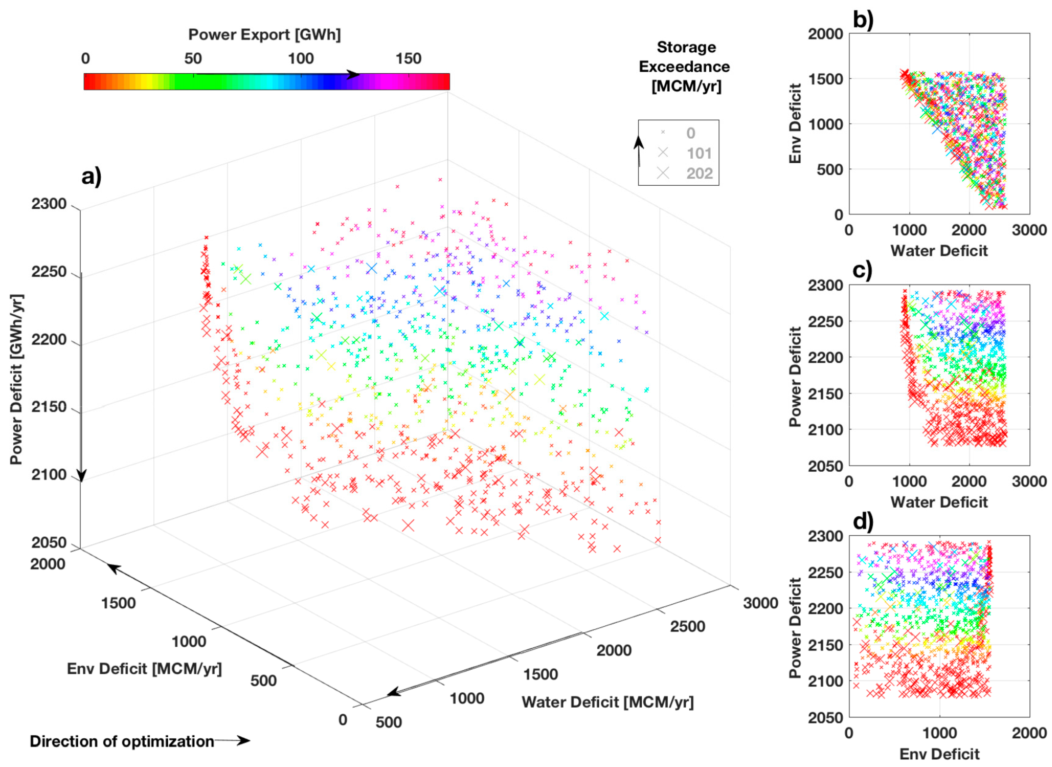
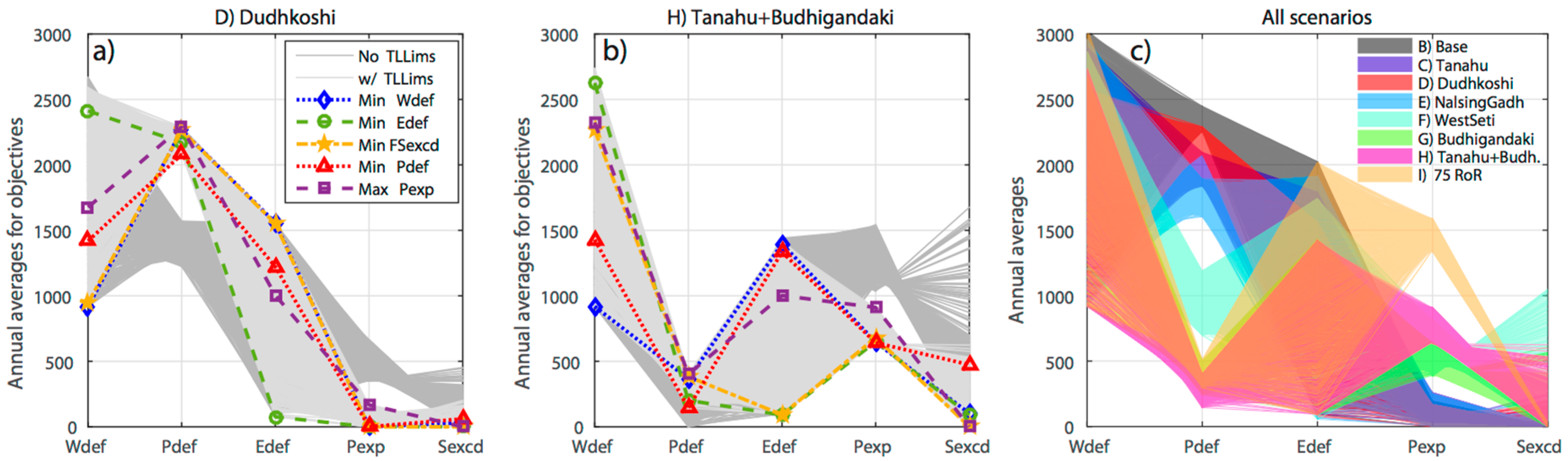
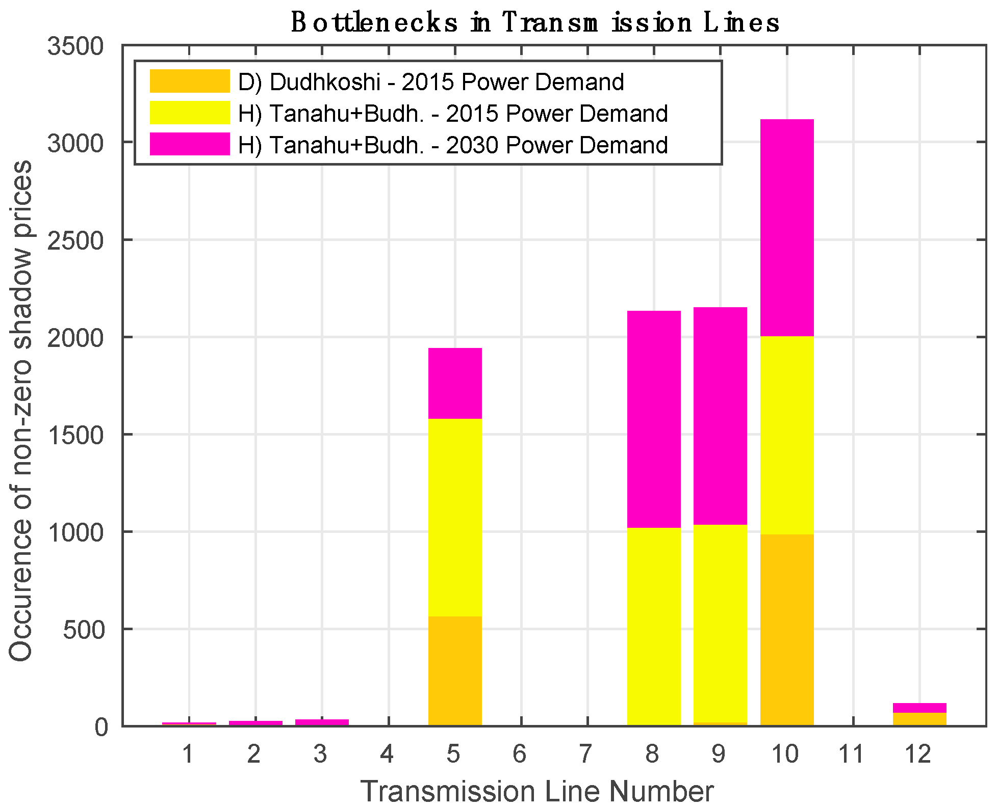
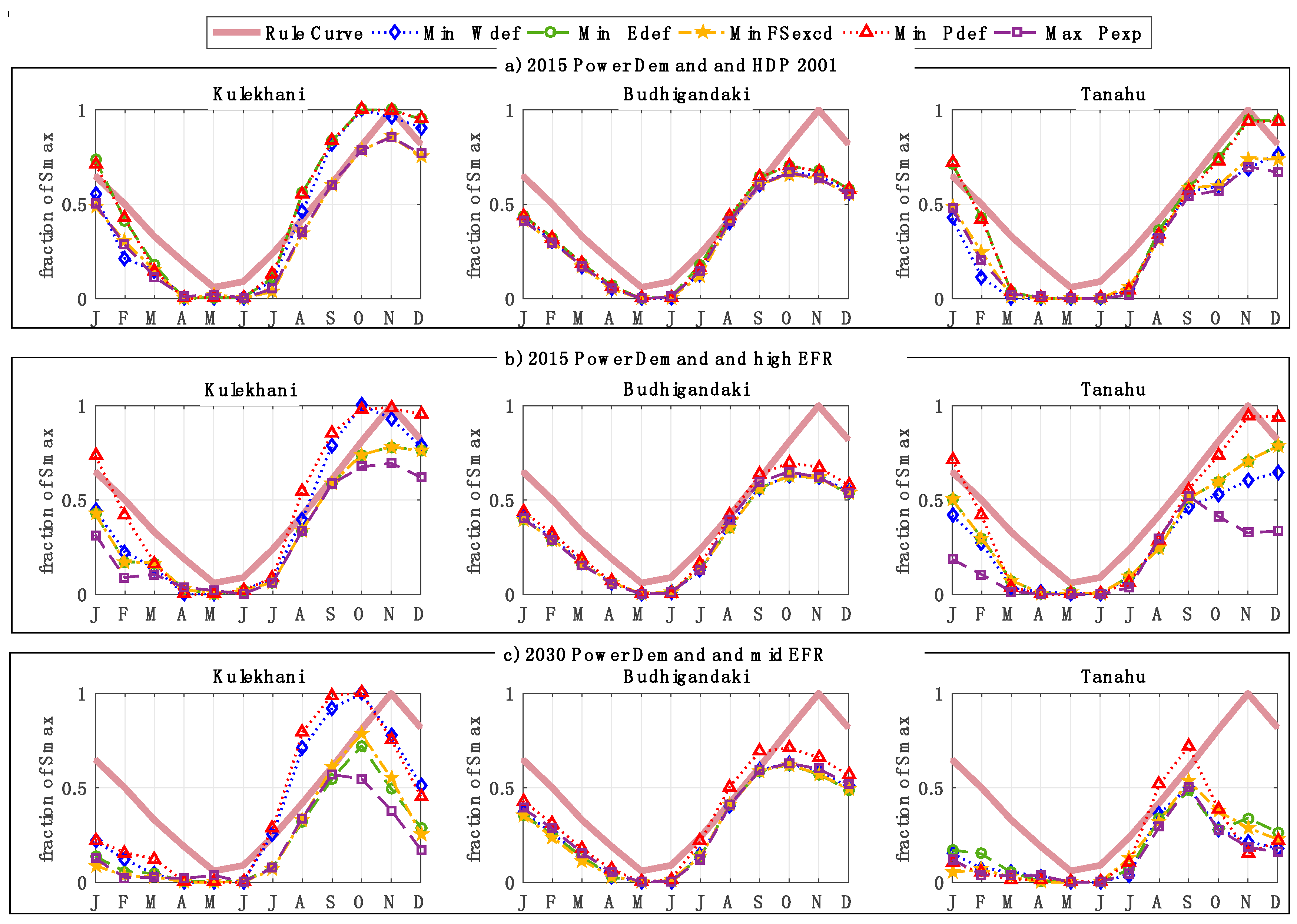
Cohon and Marks [19] and Ko et al. [94] recommend using the constraining method over the weighting method, but the constraining method can be computationally intensive if the limits to objectives are not known. To lower the number of runs required, in this study, 106 runs with weighting method are performed to determine the limits. These limits are used to further delineate the full Pareto front with 1500 runs using the constraining method. Since power and water represent resources quantified in different units, thresholds for each objective are used to normalize each deficit prior to combining them into a single function, as shown in Equation (21) for the weighting method. Such normalization is also important to ensure that the magnitudes of all performance metrics in the objective function are comparable [95].

$$\begin{array}{ll}\underset{\mathsf{\alpha }}{\min }{\Phi }_{1a}=\hfill & w_1\cdot Z_{WaterDeficit}(\mathsf{\alpha })+w_2\cdot Z_{EnvDeficit}(\mathsf{\alpha })+\dots \hfill \\ & w_3\cdot Z_{FloodRisk}(\mathsf{\alpha })+w_4\cdot Z_{PowerDeficit}(\mathsf{\alpha })\hfill \\ \mathrm{where},\forall (d,e,si,r);\hfill & t=1,\dots ,T;n_{yrs}=14;m=1,\dots ,12\hfill \\ Z_{WaterDeficit}=\hfill & \frac{1}{{\displaystyle \sum _t{\displaystyle \sum _{d}wde{m}_{d,t}}}}\cdot {\displaystyle \sum _t{\displaystyle \sum _{d}wde{f}_{d,t}}}\cdot 100\hfill \\ Z_{EnvDeficit}=\hfill & \frac{1}{{\displaystyle \sum _t{\displaystyle \sum _{e}ede{m}_{e,t}}}}\cdot {\displaystyle \sum _t{\displaystyle \sum _{e}wde{f}_{e,t}}}\cdot 100\hfill \\ Z_{FloodRisk}=\hfill & \frac{1}{{\displaystyle \sum _t{\displaystyle \sum _{si}sma{x}_{si,t}}}(1-srul{e}_{si,t})}\cdot {\displaystyle \sum _t{\displaystyle \sum _{si}sxc{d}_{si,t}}}\cdot 100\hfill \\ Z_{PowerDeficit}=\hfill & \frac{1}{{\displaystyle \sum _t{\displaystyle \sum _{r}pde{m}_r,t}}}\cdot {\displaystyle \sum _{t}pde{f}_{r,t}}\cdot 100\hfill \\ & w_1+w_2+w_3+w_4=1\hfill \end{array}$$

(21)

The constraining method is implemented by limiting three objectives and optimizing the last as follows:

$$\begin{array}{cc}& {\min }_{\mathsf{\alpha }}{\Phi }_{1b}=Z_{FloodRisk}(\mathsf{\alpha })\hfill \\ \hfill {\displaystyle \sum _t{\displaystyle \sum _{d}wde{f}_{d,t}}}\le li{m}_{wdef};& {\displaystyle \sum _t{\displaystyle \sum _{e}ede{f}_{e,t}}}\le li{m}_{edef};{\displaystyle \sum _{t}pde{f}_t}\le li{m}_{pdef}\hfill \end{array}.$$

(22)

Latin-hypercube sampling was used to generate the weights $(w_1,....,w_4)$ in Equation (21) and limits ($li{m}_{wdef},li{m}_{edef},li{m}_{pdef}$) in Equation (22).

3. Results

The proposed problem formulation resulted in large LP problems with as many as 216,384 decision variables, 72,912 inequality constraints, and 60,145 equality constraints for scenario I) with 75 new RoRs. LP proved an effective method to implement the multi-objective optimization problem even for a five-objective case with high dimensionality.

Given the variety of input parameters used to define the model and limited data availability, it is not trivial to perform a robust model validation. Figure 5 compares the actual monthly power production in 2014, estimated based on data for peak demand days in the month [57], with simulated power production for the existing scenario A) under EFR levels stipulated by the current HDP regulations. The gray lines indicate each of the 1606 model runs. Scenario A) is comparable to the 2014 power system in Nepal. However, since scenario A) excludes some seasonal plants that only operate during the high flow season, it is reasonable that the deviation between simulated and actual production is higher in the wet period (May–October) than in the dry period (November–April). Some of the simulated runs match dry period production, additionally indicating that the model provides reasonable estimates.

In Figure 5, simulated power production can be expected to be lower because model assumptions underestimate water availability. Historical discharge measured at the downstream outlets of each basin is used as representative of current water availability. The discharges observed at these downstream locations already exclude water abstracted to fulfill upstream demands. Subcatchment inflow is derived from this discharge using the fraction of basin area covered by the subcatchment, disregarding the steep terrain and heterogeneity in land cover in this region. Actual river flows observed in each subcatchment can thus be expected to be higher than assumed here. Additionally, exclusion of groundwater resources, with reported usage of 1.1 × 10⁹ m³ annually [54], and a lack of explicit accounting of potential return flows from abstracted irrigation water further propagates the underestimation of water availability. Thus, the actual tradeoffs between different water users are most likely lower than those indicated by the results presented here. However, it must be noted that the model also does not include water demand from six irrigation schemes in India that feed from the Nepalese basins [70] and ignores domestic and industrial water demand within Nepal.

Figure 6 presents the full Pareto optimal set identified for scenario D) Dudhkoshi under mid EFR with the three objectives, irrigation water deficit, environmental deficit, and power deficits, shown along the three axes, while the storage threshold exceedance is indicated by marker size and power export by marker color. It is hard to establish a distinct relation between storage threshold exceedance and other objectives. However, clear relations can be seen between the other objectives. Maximizing power export is detrimental to all national deficit minimization objectives. In the 2D views of the Pareto set, water and power deficit appear negatively correlated with higher trade-offs between the two seen for higher export in power. Power deficit and environmental deficit appear positively correlated especially for low power exports. For some combinations of export and storage threshold exceedance, scenario D) has near U-shaped contours in the power and environment deficit plot. Similar trends were observed for other scenarios but these relationships were most distinct for Dudhkoshi. Pareto sets for other scenarios from similar modeling study can be found in [55].

Visualization of multi-objective optimization results is a well-recognized challenge [24,96,97]. A parallel coordinate plot, shown in Figure 7, where multiple objectives are presented along a single horizontal axis [24], is another way to represent such data. Each light grey line in the parallel plot in Figure 7a corresponds to a scatter point on the Pareto optimal set shown in Figure 6. Figure 7b presents the plot for scenario H). The trade-off relationships are indicated by the intensity with which lines crisscross between the objectives. A high number of crossing lines indicates conflict between the objectives, while lines that do not cross indicate objectives that are in “relative harmony” [24]. Trade-off relationships can be analyzed by gathering objectives in different orders. All Pareto-optimal points are equally efficient but they can be good at fulfilling specific objectives. Five such Pareto points that fulfill each of the five objectives best are also highlighted in Figure 7a,b. The difference in objective values for the five Pareto points and intersection between the lines indicate that favoring one objective over the other in decision-making will lead to a selection of different operating policies and that trade-offs exist and they vary for different scenarios.

Figure 7a,b additionally provide a comparison of optimization results with and without inclusion of transmission line constraints in for scenarios D) and H). Figure 8 indicates identifies the transmission lines presented in Figure 4 that are limiting under these scenarios. For all other scenarios, obtained objectives had limited change between the runs with and without transmission line constraints. For scenarios G) and I), transmission lines were not limiting but the inclusion of transmission limits lowered the power deficit and export. Objective fulfillment varied most significantly with transmission limits for scenario D) because Dudhkoshi is located close to high power demand areas but with limited existing transmission lines. If transmission lines did not limit the power system performance, scenario D) would likely improve its power deficits minimization, making it a promising small storage scenario. Since storage threshold exceedance and power deficit have high tradeoffs, Figure 7a,b show that appropriate representation of line limits is also needed for realistic estimation of flood risk, especially for big reservoirs.

Parallel plots for all modeled scenarios at mid EFR are overlaid in Figure 7c; individual plots are provided in Figure S2. Due to the smaller range of power deficit and export in comparison to the water and environmental deficit, it is hard to see the intensity of intersections between the lines. Nevertheless, this indicates that changing reservoir operation for small improvements in power deficit can have big impacts on the water objectives. The relationships vary for all scenarios, but generally, there is a trade-off between power and water deficit while environmental deficit, power deficit, and power export are in relative harmony. Figure 7c also shows that despite providing higher HP capacity addition than the two new storages in scenario H), scenario I) with no new reservoir results in higher power deficits. Instead scenario H) results in improved power export at higher environmental deficits.

Figure 9 compares the Pareto optimal solution set for scenario H) run with the current HDP and all three levels of EFR. Imposing up to mid-level EFR at outflow nodes brings limited change to power deficits. As environmental deficit and water deficit have strong negative correlation, high EFR requirement increases both deficits, which in turn worsens the flood risk objective. High EFR results in slightly higher power exports suggesting that imposing higher EFR potentially increases power production in some basins but directs more power out of Nepal due to the transmission line constraints. This interplay between basin-wise power production and inter-basin transmission constraint is important for establishing national EFR levels.

Figure 10 presents the monthly variation in objectives at five Pareto optimal points for scenarios B), D), F), and I). The average monthly variation over the 14-year simulation period in power deficit, water deficit, and reservoir storages in fractions are presented. Both water and power deficits do not vary much for the five Pareto points in the wet period. Trends in water deficit and environmental deficits are opposite, so only water deficits are shown here. With successive addition of new reservoirs, there is more flexibility and hence trade-offs in operating the existing Kulekhani reservoir. Under scenarios B) and I), operation of Kulekhani has relatively limited flexibility where wet period reservoir release is required for all points except minimization of water deficits. Scenario D) does not allow much flexibility in operation of the new Dudhkoshi reservoir, but its addition allows Kulekhani to either carry over wet period flow to minimize dry period power and water deficit or release it for current power export and EFRs. Similar trade-offs have to be made in both Kulekhani and West Seti reservoir when operating the two plants simultaneously in scenario F). Meeting both dry-period irrigation and power deficit requires water to be stored so scenario I) with only new RoRs cannot lower the water deficit compared to the scenario B). Instead, water deficit is worsened as water is not allocated to irrigation nodes upstream of RoR turbine nodes. Scenarios G) and H) (not shown here) have similar trend to scenario D), while scenarios C) and E) show variation in reservoir operations similar to scenario F).

Figure 11 compares the operation of Kulekhani, Budhiganadki, and Tanahu in scenario H), when run with different EFRs and higher power demand for 2030. In Figure 11a,b, the operation of Kulekhani varies more in the dry period than it did in the scenarios in Figure 10 Since the two-storage scenario represents a big power upgrade that can easily reduce the power deficit to zero, the optimizer can focus on fulfilling other objectives. The higher EFR scenario can also be considered similar to a case accounting for Indian irrigation water demand occurring downstream of Nepalese river basins. The difference in reservoir operation for the two EFR levels can indicate the conflicts in water sharing between the two countries. Once power demand is higher again in Figure 11c, the variation in operation is similar again for the dry months. Increase in power demand results in reservoir accumulation and release beginning earlier for all three reservoirs. Operation policy for Tanahu changes significantly from dry-season, production-based to year-round production as the scenario is no longer able to fulfill wet-period power demands for 2030.

4. Discussion

This study evaluated Pareto fronts for different hydropower development scenarios in Nepal assuming perfect foresight with deterministic historical inflows, constant power and water demands, fixed storage rule curves, and fixed hydropower production capacities. The impact of uncertainties in input parameters and linear representation of nonlinearity in water and power systems has not been formally addressed. The use of a variety of demand scenarios provides some basis for discussing sensitivities, but a rigorous analysis similar to that undertaken by [98,99,100] or [101], where parameter uncertainties are characterized using probability distributions for constraints and thresholds, should be addressed by future work. Nonetheless, this study provides a good basis for screening alternatives with a broader understanding of both the Nepalese water–energy–food nexus itself and the performance of proposed alternative with regards to the diverse nexus objectives. It is demonstrated that multi-objective optimization can provide a flexible and thorough means to evaluate infrastructure development plans using the nexus approach. The spatial disaggregation allows for intuitive evaluation of each reservoir individually that is usually not possible in lumped optimization models. The parallel plots and monthly variation curves evaluated in the study provide many insights to help decision makers make informed choices to shortlist candidate project for further analysis in more complex and detailed models [102].

Multi-objective optimization models and interdependencies revealed by visual analysis of Pareto frontiers are useful to overcome two forms of bias inherent in human decision making processes [31,102]. ‘Cognitive hysteresis’ refers to the bias in problem definitions itself due to decision maker’s pre-conceptions regarding the nature of the problem or its objectives, while ‘cognitive myopia’ refers to the challenge of not identifying or including innovative solutions due to narrow problem definitions. The nexus approach to assist power development studies proposed here helps overcome these two biases by assessing performance of power development scenarios under objectives of direct interest to government power planners (power deficit and power export) and objectives of interest to other stakeholders that are affected by hydropower development (irrigation water deficit, flood risk exceedance, and environmental deficit). Figure 5 confirms that various model assumptions and the use of historical discharge at downstream outlets results in an underestimation of water availability and subsequent power production. The use of the same reservoir storage rule curve for all storage plants is another data limitation. The dimensions of the reservoirs and their drainage areas vary significantly. Based on geographic location of the plants, flood magnitude and frequency will also vary across basins. The location of the reservoirs within each basin also changes the relationships between upstream and downstream water users. Since irrigation water demands are generally higher in the southern plains, reservoirs located closer to the south will see greater conflict in reservoir operation. These factors stipulate the need for unique reservoir operation policy for each storage plant. The poor quantification of reservoir storage rule curves in turn makes the performance metric used for flood risk minimization debatable. A potential future extension could be inclusion of the reservoir operation policy as a decision variable as done by Geressu and Harou [103]. Deriving rule curves through such coupled simulation could further maximize the observed synergies between the reservoirs. However, a different metric for flood risk quantification will be needed in that case.

Comparing trend in Figure 7 and Figure 9 with that in Figure 10, it can be noted that the annual averages for water deficits are dominated by the naturally high deficits in the dry months. In the dry period, all objectives require reservoir releases. In the wet period, some objectives require storage while some require release, which shapes the monthly trade-offs in reservoir operation. Therefore, the patterns in trade-offs seen at annual levels in Figure 6, Figure 7, Figure 8 and Figure 9 are not the same for trade-offs seen in monthly operation in Figure 10 and Figure 11. It may be worthwhile evaluating national trade-offs for the wet and dry period separately as annual scale Pareto fronts may be misleading.

The use of a coupled model, as presented here, allows for a holistic comparison of scenario performance under metrics for not only power and water resource utilization but also overall system efficiency. The approach also allows for comparison of scenarios based on compatibility with existing transmission network while identifying critical links in the system. For instance, in Figure 7a, while Dudhkoshi performs well in terms of water and environmental deficit, its full power potential is not explored when transmission constraints are placed on the system.

Three different EFR levels were used as inputs in this case study. Using the same setup, this framework can also be used for scenario-based EFR setting [79] by helping authorities understand the change in trade-offs from establishing EFRs based on different methods.

The modeling demonstration here presented an analysis of the water–energy–food nexus from the perspective of power development in Nepal. A similar analysis from the perspective of irrigation and water supply infrastructure development scenarios could also be implemented using the same model setup. The current model has irrigation water demand as the only parameter representing the food sector. An application focusing on food security assessment should consider connecting the presented coupled water–power model to a linear crop model at the irrigation nodes for a more rigorous representation of food production. Coupling with non-linear crop models would require using non-linear solvers or evolutionary algorithms.

While the model is spatially explicit, the results have been analyzed at an aggregated national scale. Basin scale analysis, as done by Hurford et al. [17] for the Brazilian Jaguaribe basin, is not included here because the lack of a pre-defined metric (e.g., curtailment costs, seniority rights) to set the preference for power and water demand fulfillment across the various nodes allows for multiple allocation possibilities. Since node-wise allocations are currently dictated by the heuristics of the LP solver, inter-basin, and subcatchment scale analysis and may not be reliable, they are not presented. With additional input from decision makers regarding preference in demand fulfillment, the proposed model could also be extended to explore inter-basin social dynamics and livelihood impacts objectives. Projects like West Seti and Nalsing Gad, located in less-developed regions of Nepal, could benefit from such evaluation.

Insights for Hydropower Development in the Nepalese Nexus

It is clear from the trade-offs between the power and water objectives seen in Figure 6, Figure 7, Figure 8, Figure 9, Figure 10 and Figure 11 that the current notion of no conflict is not true and trade-offs will change as more HP plants are added to the system. It is hard to generalize the inter-dependencies between the nexus objectives across all development plans as each new storage plant is in a different basin and each basin presents its own tradeoffs. Nonetheless, it is seen that meeting power demands for the dry period presents conflicts in monthly reservoir management. Increase in power demands or EFRs also changes the trade-offs, with operations under the five different management objectives showing more variation if production capacity is comparable to power demand. Export-oriented reservoir operation will lower the amount of water available for crop production, while minimizing these irrigation deficits will affect the amount of water available for both power production and support of the ecosystem. For most scenarios, annual power deficit is in harmony with environmental deficit as reservoir releases help fulfill both objectives simultaneously.

It is observed in Figure 7a that hydropower expansion strictly based on RoRs will result in significant conflicts in monthly irrigation water allocation and will not lower power deficits as much as storage projects with lower added capacities. Storage scenarios are more promising options for concurrent reduction in power deficit and fulfillment of other management objectives. Figure 7c shows that the smaller storage plants in scenarios C), D), and E) are not good for export but scenario D) can lower water and environmental deficits even more than the bigger scenarios, E) and F). Also, when comparing the relative performance of Tanahu, Budhigandaki, and the two reservoirs together, implementing only Budhigandaki may be sufficient. Different reservoirs like Kulekhani and Tanahu offer varying trade-offs between the minimization of power and irrigation water deficit as additional plants are available to produce power in the wet period. Dudhkoshi and Budhigandaki do not seem to offer such flexibility in the scenarios modeled here. However, their operational flexibility can change if new plants are added, as seen here for the case of Kulekhani and Tanahu. In terms of system compatibility, existing transmission lines can support most of the modeled scenarios, but increasing connectivity between the eastern and central distribution regions will help maximize power production and fulfill the high power demands in the central regions.

Considering the reservoir operation at the five Pareto-optimal policies under all scenarios shown in Figure 10 and Figure 11, operating at the Pareto point minimizing power deficit is critical because it requires higher wet-period reservoir storage than other points. If the focus of the government remains on minimizing power deficit, the water needs of the environment or irrigation users in the dry period may not be served. Placing various levels of EFR at basin outflow points did not have any evident impact on annual power deficits in Figure 9. Therefore, imposing EFRs may be justified as a means to secure non-power water users in the wet period. Since this analysis has been done from the perspective of Nepal and ignores water users further downstream in India, the high EFR scenarios can also be taken as proxies for including Indian water demands in the model. Even if there are limited conflicts with fulfilling internal power and water demands, adding demands from India will result in significant trade-offs and conflicts. Establishing basin-scale EFR requirements may eventually pave the path to allocating EFR downstream of each hydropower plant.

5. Conclusions

A coupled and disaggregated multi-objective optimization model has been developed to analyze various aspects of the water–energy–food nexus under the constraints placed by natural water availability, power transmission network, upstream–downstream nexus linkages, and environmental flow requirements. The framework combines two well-established water and power system models while focusing on the need for finer spatial representation to accurately model the interactions in the nexus. The proposed modeling framework is demonstrated on the water–energy–food nexus for Nepal and used to successfully characterize the full Pareto sets for eight power development scenarios under four levels of EFRs and two power demands. It has been demonstrated that decision biases can arise from lumped representation of water systems and this framework embodying the nexus approach can provide broader insights for well-informed decision-making. The delineated Pareto optimal solution sets allow for comparison of both the different development scenarios and operation policies available within each scenario. Thus, the method is particularly valuable in cases where limited knowledge is available regarding a decision maker’s preferences for objective fulfillment. By visualizing all possible optimal solutions under each scenario, the method can help the divided sectors in the government recognize ways to combine their goals by understanding the consequences of power development on other sectors. Poor data availability and subsequent assumptions limit the model performance as applied to the Nepalese hydropower development case here. The matrix-based flow path representation of the system allows for easy setup and replication of the model for a data-rich case. Disaggregated linear multi-objective optimization is a promising approach for combining more than just the water and power system models coupled here to address other aspects of the water–energy–food nexus and beyond.

References

1. Weitz, N.; Huber-Lee, A.; Nilsson, M.; Davis, M.; Hoff, H. Cross-Sectoral Integration in the Sustainable Development Goals: A Nexus Approach; Stockholm Environment Institute: Stockholm, Sweden, 2014. [Google Scholar]
2. Hoff, H. Understanding the Nexus. In Background Paper for the Bonn2011 Conference: The Water, Energy and Food Security Nexus; Stockholm Environment Institute: Stockholm, Sweden, 2011. [Google Scholar]
3. Bazilian, M.; Rogner, H.; Howells, M.; Hermann, S.; Arent, D.; Gielen, D.; Steduto, P.; Mueller, A.; Komor, P.; Tol, R.S.J.; et al. Considering the energy, water and food nexus: Towards an integrated modelling approach. Energy Policy 2011, 39, 7896–7906. [Google Scholar] [CrossRef]
4. Suhardiman, D.; Clement, F.; Bharati, L. Integrated water resources management in Nepal: Key stakeholders’ perceptions and lessons learned. Int. J. Water Resour. Dev. 2015, 31, 284–300. [Google Scholar] [CrossRef]
5. Biggs, E.M.; Duncan, J.M.A.; Atkinson, P.M.; Dash, J. Plenty of water, not enough strategy. How inadequate accessibility, poor governance and a volatile government can tip the balance against ensuring water security: The case of Nepal. Environ. Sci. Policy 2013, 33, 388–394. [Google Scholar] [CrossRef]
6. Rasul, G. Managing the food, water, and energy nexus for achieving the sustainable development goals in South Asia. Environ. Dev. 2015, 18, 1–12. [Google Scholar] [CrossRef]
7. Allouche, J.; Middleton, C.; Gyawali, D. Nexus Nirvana or Nexus Nulity? A Dynamic Approach to Security and Sustainability in the Water-Energy-Food Nexus; STEPS Working Paper 63; STEPS Centre: Brighton, UK, 2014. [Google Scholar]
8. Leck, H.; Conway, D.; Bradshaw, M.; Rees, J. Tracing the water-energy-food nexus: Description, theory and practice. Geogr. Compass 2015, 9, 445–460. [Google Scholar] [CrossRef]
9. Benson, D.; Gain, A.K.; Rouillard, J.J. Water governance in a comparative perspective: From IWRM to a “nexus” approach? Water Altern. 2015, 8, 756–773. [Google Scholar]
10. Gyawali, D. Nexus Governance: Harnessing Contending Forces at Work; International Water Association: London, UK, 2015. [Google Scholar]
11. Bizikova, L.; Roy, D.; Swanson, D.; Venema, H.D.; McCandless, M. The Water-Energy-Food Security Nexus: Towards a Practical Planning and Decision-Support Framework for Landscape Investment and Risk Management; International Institute for Sustainable Development: Winnipeg, MB, Canada, 2013. [Google Scholar]
12. Flammini, A.; Puri, M.; Pluschke, L.; Dubois, O. Walking the Nexus Talk: Assessing the Water-Energy-Food Nexus in the Context of the Sustainable Energy for All Initiative; Food and Agriculture Organization: Rome, Italy, 2014. [Google Scholar]
13. Kumar, N.; Gerber, N. Approaches to Resource Management for the Nexus. Chang. Adapt. Socio-Ecol. Syst. 2015, 2. [Google Scholar] [CrossRef]
14. Howells, M.; Hermann, S.; Welsch, M.; Bazilian, M.; Segerström, R.; Alfstad, T.; Gielen, D.; Rogner, H.; Fischer, G.; van Velthuizen, H.; et al. Integrated analysis of climate change, land-use, energy and water strategies. Nat. Clim. Chang. 2013, 3, 621–626. [Google Scholar] [CrossRef]
15. Giampietro, M.; Aspinall, R.J.; Bukkens, S.G.F.; Benalcazar, J.C.; Diaz-Maurin, F.; Flammini, A.; Gomiero, T.; Kovacic, Z.; Madrid, C.; Ramos-Martin, J.; et al. An Innovative Accounting Framework for the Food-Energy-Water Nexus: Application of the MuSIASEM Approach to Three Case Studies; Food and Agriculture Organization: Rome, Italy, 2013. [Google Scholar]
16. Hurford, A.P.; Harou, J.J. Balancing ecosystem services with energy and food security – Assessing trade-offs from reservoir operation and irrigation investments in Kenya’s Tana Basin. Hydrol. Earth Syst. Sci. 2014, 18, 3259–3277. [Google Scholar] [CrossRef]
17. Hurford, A.P.; Huskova, I.; Harou, J.J.; Wallingford, H.R.; Park, H.; Lane, B.; Ox, W. Using many-objective trade-off analysis to help dams promote economic development, protect the poor and enhance ecological health. Environ. Sci. Policy 2013, 38, 72–86. [Google Scholar] [CrossRef]
18. Haimes, Y.Y.; Hall, W.A. Sensitivity, responsivity, stability and irreversibility as multiple objectives in civil systems. Adv. Water Resour. 1977, 1, 71–81. [Google Scholar] [CrossRef]
19. Cohon, J.L.; Marks, D.H. A review and evaluation of multiobjective programing techniques. Water Resour. Res. 1975, 11, 208–220. [Google Scholar] [CrossRef]
20. Loucks, D.P.; van Beek, E.; Stedinger, J.R.; Dijkman, J.P.M.; Villars, M.T. Water Resources Systems Planning and Management: An Introduction to Methods, Models and Applications; The United Nations Educational, Scientific and Cultural Organization: Delft, Netherlands, 2005. [Google Scholar]
21. Brown, C.M.; Lund, J.R.; Cai, X.; Reed, P.M.; Zagona, E.A.; Ostfeld, A.; Hall, J.; Characklis, G.W.; Yu, W.; Brekke, L. The future of water resources systems analysis: Toward a scientific framework for sustainable water management. Water Resour. Res. 2015, 51, 6110–6124. [Google Scholar] [CrossRef]
22. Maass, A.; Hufschmidt, M.M.; Dorfman, R.; Harold, A.; Thomas, J.; Marglin, S.A.; Fair, G.M. Design of Water-Resource Systems: New Techniques for Relating Economic Objectives, Engineering Analysis, and Governmental Planning; Harvard University Press: Cambridge, MA, USA, 1962. [Google Scholar]
23. Cohon, J.L. Multiobjective Programming and Planning; Courier Corporation: North Chelmsford, MA, USA, 1978; Volume 140. [Google Scholar]
24. Fleming, P.J.; Purshouse, R.C.; Lygoe, R.J.; Street, M. Many-objective optimization: An engineering design perspective. In Evolutionary Multi-Criterion Optimization; Coello, C.A.C., Aguirre, A.H., Zitzler, E., Eds.; Springer: Berlin/Heidelberg, Germany, 2005; Volume 3410, pp. 14–32. [Google Scholar]
25. Coello, C.A.C.; Lamont, G.B.; van Veldhuizen, D.A. Evolutionary Algorithms for Solving Multi-Objective Problems; Springer: Berlin/Heidelberg, Germany, 2007. [Google Scholar]
26. Yeh, W.W.-G. Reservoir Management and Operations Models: A State of the Art Review. Water Resour. Res. 1985, 21, 1797–1818. [Google Scholar] [CrossRef]
27. Harou, J.J.; Pulido-Velazquez, M.; Rosenberg, D.E.; Medellín-Azuara, J.; Lund, J.R.; Howitt, R.E. Hydro-economic models: Concepts, design, applications, and future prospects. J. Hydrol. 2009, 375, 627–643. [Google Scholar] [CrossRef]
28. Labadie, J.W. Optimal operation of multireservoir systems: State-of-the-art review. J. Water Resour. Plan. Manag. 2004, 130, 93–111. [Google Scholar] [CrossRef]
29. Maier, H.R.; Kapelan, Z.; Kasprzyk, J.R.; Kollat, J.; Matott, L.S.; Cunha, M.C.; Dandy, G.C.; Gibbs, M.S.; Keedwell, E.; Marchi, A.; et al. Evolutionary algorithms and other metaheuristics in water resources: Current status, research challenges and future directions. Environ. Model. Softw. 2014, 62, 271–299. [Google Scholar] [CrossRef] [Green Version]
30. Nicklow, J.; Asce, F.; Reed, P.; Asce, M.; Savic, D.; Dessalegne, T.; Harrell, L.; Chan-Hilton, A.; Karamouz, M.; Minsker, B.; et al. State of the Art for Genetic Algorithms and Beyond in Water Resources Planning and Management. J. Water Resour. Plan. Manag. 2010, 136, 412–432. [Google Scholar] [CrossRef]
31. Reed, P.M.; Hadka, D.; Herman, J.D.; Kasprzyk, J.R.; Kollat, J.B. Evolutionary multiobjective optimization in water resources: The past, present, and future. Adv. Water Resour. 2013, 51, 438–456. [Google Scholar] [CrossRef]
32. Salazar, J.Z.; Reed, P.M.; Herman, J.D.; Giuliani, M.; Castelletti, A. A diagnostic assessment of evolutionary algorithms for multi-objective surface water reservoir control. Adv. Water Resour. 2016, 92, 172–185. [Google Scholar] [CrossRef]
33. Tekiner, H.; Coit, D.W.; Felder, F.A. Multi-period multi-objective electricity generation expansion planning problem with Monte-Carlo simulation. Electr. Power Syst. Res. 2010, 80, 1394–1405. [Google Scholar] [CrossRef]
34. Chen, F.; Huang, G.; Fan, Y. A linearization and parameterization approach to tri-objective linear programming problems for power generation expansion planning. Energy 2015, 87, 240–250. [Google Scholar] [CrossRef]
35. Aghaei, J.; Akbari, M.A.; Roosta, A.; Baharvandi, A. Multiobjective generation expansion planning considering power system adequacy. Electr. Power Syst. Res. 2013, 102, 8–19. [Google Scholar] [CrossRef]
36. Bakirtzis, G.A.; Biskas, P.N.; Chatziathanasiou, V. Generation expansion planning by MILP considering mid-term scheduling decisions. Electr. Power Syst. Res. 2012, 86, 98–112. [Google Scholar] [CrossRef]
37. Castelletti, A.; Pianosi, F.; Restelli, M. A multiobjective reinforcement learning approach to water resources systems operation: Pareto frontier approximation in a single run. Water Resour. Res. 2013, 49, 3476–3486. [Google Scholar] [CrossRef]
38. World Commission on Dams. Dams and Development: A New Framework for Decision-Making; Earthscan Publications: London, UK, 2000. [Google Scholar]
39. Karlberg, L.; Hoff, H.; Amsalu, T.; Andersson, K.; Binnington, T.; Flores-López, F.; de Bruin, A.; Gebrehiwot, S.G.; Gedif, B.; zur Heide, F.; et al. Tackling complexity: Understanding the food-energy-environment nexus in Ethiopia’s lake TANA sub-basin. Water Altern. 2015, 8, 710–734. [Google Scholar]
40. Jalilov, S.M.; Keskinen, M.; Varis, O.; Amer, S.; Ward, F.A. Managing the water-energy-food nexus: Gains and losses from new water development in Amu Darya River Basin. J. Hydrol. 2016, 539, 648–661. [Google Scholar] [CrossRef]
41. Briscoe, J. The Financing of Hydropower, Irrigation and Water Supply Infrastructure in Developing Countries. Int. J. Water Resour. Dev. 1999, 15, 459–491. [Google Scholar] [CrossRef]
42. Richter, B.D.; Postel, S.; Revenga, C.; Scudder, T.; Lehner, B.; Churchill, A.; Chow, M. Lost in development’s shadow: The downstream human consequences of dams. Water Altern. 2010, 3, 14–42. [Google Scholar]
43. Biemans, H.; Siderius, C.; Mishra, A.; Ahmad, B. Crop-specific seasonal estimates of irrigation water demand in South Asia. Hydrol. Earth Syst. Sci. Discuss. 2015, 12, 7843–7873. [Google Scholar] [CrossRef]
44. Rasul, G. Food, water, and energy security in South Asia: A nexus perspective from the Hindu Kush Himalayan region. Environ. Sci. Policy 2014, 39, 35–48. [Google Scholar] [CrossRef]
45. Biemans, H.; Siderius, C.; Mishra, A.; Ahmad, B. Crop-specific seasonal estimates of irrigation-water demand in South Asia. Hydrol. Earth Syst. Sci. 2016, 20, 1971–1982. [Google Scholar] [CrossRef]
46. Wood, A.J.; Wollenberg, B.F. Optimal Power Flow. In Power Generation, Operation, and Control; John Wiley & Sons: New York, NY, USA, 1996; Volume 37. [Google Scholar]
47. Cheng, W.-C.; Hsu, N.-S.; Cheng, W.-M.; Yeh, W.W.-G. A flow path model for regional water distribution optimization. Water Resour. Res. 2009, 45, 1–12. [Google Scholar] [CrossRef]
48. DesInventar Project Team DesInventar—Profile: Nepal. Available online: http://www.desinventar.net/DesInventar/profiletab.jsp?countrycode=npl (accessed on 18 August 2015).
49. Ministry of Water Resources. The Hydropower Development Policy, 2001; Singha Durbar: Kathmandu, Nepal, 2001.
50. Water and Energy Commission Secretariat. National Water Plan—Nepal; Department of Soil Conservation and Watershed Management: Kathmandu, Nepal, 2005.
51. Jarvis, A.; Reuter, H.I.; Nelson, A.; Guevara, E. Hole-filled seamless SRTM data V4. Available online: http://srtm.csi.cgiar.org (accessed on 20 August 2015).
52. Department of Electricity Development Issued Licenses. Available online: http://www.doed.gov.np/issued_licenses.php (accessed on 15 September 2015).
53. Rijal, N.; Paragon Engineering Consultancy and Research Centre, Lalitpur, Nepal. Personal Communication, 2015.
54. Asian Development Bank; International Center for Integrated Mountain Development. Environment Assessment of Nepal Emerging Issues and Challenges; Mountain Forum: Kathmandu, Nepal, 2006. [Google Scholar]
55. Dhaubanjar, S. Multiobjective Optimisation for Water Resources Management in Nepal. Master’s Thesis, Department of Environmental Engineering, Technical University of Denmark (DTU), Lyngby, Denmark, 2016. [Google Scholar]
56. Nepal Electricity Authority. A Year in Review: Fiscal Year 2014/2015; Nepal Electricity Authority: Kathmandu, Nepal, 2015.
57. Shrestha, M.; Load Dispatch Center, Nepal Electricity Authority, Kathmandu, Nepal. Personal Communication, 2015.
58. Nepal Electricity Authority. Load Forecast Report; Nepal Electricity Authority: Kathmandu, Nepal, 2015.
59. Central Bureau of Statistics. Statistical Year Book of Nepal 2013; Central Bureau of Statistics: Kathmandu, Nepal, 2013.
60. Agri-Business Promotion and Statistics Division. Statistical Information on Nepalese Agriculture: Time Series Information 1999/2000-2011/2012; Agri-Business Promotion and Statistics Division: Kathmandu, Nepal, 2013.
61. Fang, C.; Sharma, R.; Favre, R.; Hollema, S. Food Security Assessment Mission to Nepal; UN Nepal Information Platform: Nepalgunj, Nepal, 2007. [Google Scholar]
62. Nepal National Committee of International Committe of Irrigation and Drainage Nepal. Available online: http://www.icid.org/v_nepal.pdf (accessed on 9 July 2015).
63. Food and Agriculture Organization of the United Nations. Irrigation Water Requirement and Water Withdrawal by Country; Food and Agriculture Organization of the United Nations: Rome, Italy, 2012. [Google Scholar]
64. Water and Energy Commission Secretariat. Water Resources of Nepal in the Context of Climate Change; Water and Energy Commission Secretariat: Kathmandu, Nepal, 2011. [Google Scholar]
65. Thapa, G. Govt Introduces Household Solar System Scheme; Kathmandu Post: Kathmandu, Nepal, 2015. [Google Scholar]
66. The Himalayan Times. Load Shedding Time Increases upto 14 Hrs a Day; The Himalayan Times: Kathmandu, Nepal, 2016. [Google Scholar]
67. Ministry of Energy. 20-Year Hydropower Development Task Force Report; Ministry of Energy: Kathmandu, Nepal, 2009. (In Nepali)
68. Sharma, R.H.; Awal, R. Hydropower development in Nepal. Renew. Sustain. Energy Rev. 2013, 21, 684–693. [Google Scholar] [CrossRef]
69. Giri, S. Govt Estimates 200 MW Can Be Added to Grid This Year; Kathmandu Post: Kathmandu, Nepal, 2015. [Google Scholar]
70. Japan International Cooperation Agency; Nepal Electricity Authority. Nationwide Master Plan Study on Storage-Type Hydroelectric Power Development in Nepal: Strategic Environmental Impact Assessment Report; Nepal Electricity Authority: Kathmandu, Nepal, 2014.
71. Bajracharya, I. Assessment of Run-of-River Hydropower Potential and Power Supply Planning in Nepal Using Hydro Resources; Technischen Universität Wien: Vienna, Austria, 2015. [Google Scholar]
72. Hada, R.P. Kulekhani reservoir: Our operational experience. In Hydropower in the New Millennium, Proceedings of the 4th International Conference Hydropower, Bergen, Norway, 20–22 June 2001; Honningsvag, B., Midttomme, G.H., Repp, K., Vaskinn, K., Westeren, T., Eds.; CRC Press: Bergen, Norway, 2001; pp. 75–84. [Google Scholar]
73. Tanahu Hydropower Limited Salient Features: Tanahu Hydropower Project. Available online: http://thl.com.np/index.php?nav=salient (accessed on 17 January 2016).
74. Nalsing Gad Hydropower Development Committee Salient Features: Nalsing Gad Hydropower Project. Available online: http://www.nhpdc.gov.np/salient-features.php (accessed on 17 August 2015).
75. CWE Investment Corp. West Seti Hydropower Project in Nepal: Technical Evaluation; CWE Investment Corp: Kathmandu, Nepal, 2013. [Google Scholar]
76. Project Development Department. Budhi Gandaki Hydroelectric Project: Review Report; Roject Development Department: Kathmandu, Nepal, 2011.
77. Poff, N.L.; Allan, J.D.; Bain, M.B.; Karr, J.R.; Prestegaard, K.L.; Richter, B.D.; Sparks, R.E.; Stromberg, J.C. The natural flow regime: A paradigm for river conservation and restoration. Bioscience 1997, 47, 769–784. [Google Scholar] [CrossRef]
78. Tennant, D.L. Instream Flow Regimens for Fish, Wildlife, Recreation and Related Environmental Resources. Fisheries 1976, 1, 6–10. [Google Scholar] [CrossRef]
79. Acreman, M.C.; Dunbar, M.J. Defining environmental river flow requirements—A review. Hydrol. Earth Syst. Sci. 2004, 8, 861–876. [Google Scholar] [CrossRef]
80. Smakhtin, V.U.; Shilpakar, R.L.; Hughes, D.A. Hydrology-based assessment of environmental flows: An example from Nepal. Hydrol. Sci. J. 2006, 51, 207–222. [Google Scholar] [CrossRef]
81. Flow: The Essentials of Environmental Flows; Dyson, M.; Bergkamp, G.; Scanlon, J. (Eds.) International Union for Conservation of Nature and Natural Resources: Gland, Switzerland; Cambridge, UK, 2003; Volume 1.
82. Rai, R.K.; Upadhyay, A.; Ojha, C.S.P.; Singh, V.P. Environmental Flows. In The Yamuna River Basin; Springer: Dordrecht, The Netherlands, 2012; Volume 66, pp. 357–406. [Google Scholar]
83. Smakhtin, V.U.; Shilpakar, R.L. Planning for Environmental Water Allocations: An Example of Hydrology-Based Assessment in the East Rapti River, Nepal; Research Report 89; International Water Management Institute: Colombo, Sri Lanka, 2005. [Google Scholar]
84. Smakhtin, V.U.; Anputhas, M. An Assessment of Environmental Flow Requirements of Indian River Basins; Research Report 107; International Water Management Institure: Colombo, Sri Lanka, 2006. [Google Scholar]
85. Shrestha, A.B.; Wake, C.P.; Mayewski, P.A.; Dibb, J.E. Maximum Temperature Trends in the Himalaya and Its Vicinity : An Analysis Based on Temperature Records from Nepal for the Period 1971–94. J. A. Meteorol. Soc. 1999, 12, 2775–2786. [Google Scholar] [CrossRef]
86. Shrestha, M.L.; Shrestha, A.B. Recent trends and potential climate change impacts on glacier retreat/lakes in Nepal and potential adaptation. In Global Forum on Sustainable Development: Development and Climate Change; Department of Hydrology and Meterology: Paris, France, 2004. [Google Scholar]
87. Shrestha, S.; Khatiwada, M.; Babel, M.S.; Parajuli, K. Impact of Climate Change on River Flow and Hydropower Production in Kulekhani Hydropower Project of Nepal. Environ. Process. 2014, 1, 231–250. [Google Scholar] [CrossRef]
88. Nepal Development Research Institute (NDRI); Practical Action Consulting (PAC); Global Adaptation Partnership (GCAP). Adaptation to Climate Change in the Electricity Sector in Nepal: Vulnerability Assessment Report (Draft); Nepal Development Research Institute (NDRI): Kathmandu, Nepal, 2016. [Google Scholar]
89. Nepal Electricity Authority. A Year in Review: Fiscal Year 2013/2014; Nepal Electricity Authority: Kathmandu, Nepal, 2014.
90. Shrestha, P. Cross-Border Transmission Line between Nepal and India: A Test-Case for the Analysis of HVDC Integration into an Existing HVAC System. Master’s. Thesis, Norwegian University of Science and Technology (NTNU), Trondheim, Norway, 2016. [Google Scholar]
91. IBM Corporations ILOG CPLEX Optimization Studio 12.6.1. Available online: https://www.ibm.com/support/knowledgecenter/en/SSSA5P_12.6.1/ilog.odms.studio.help/Optimization_Studio/topics/COS_home.html (accessed on 5 January 2016).
92. Seifi, H.; Sepasian, M.S. DC Load Flow. In Electric Power System Planning: Issues, Algorithms and Solutions; Springer Science & Business Media: Berlin/Heidelberg, Germany, 2011; pp. 245–248. [Google Scholar]
93. Molzahn, D.K.; Friedman, Z.B.; Lesieutre, B.C.; DeMarco, C.L.; Ferris, M.C. Estimation of Constraint Parameters in Optimal Power Flow Data Sets. In Proceedings of the 2015 North American Power Symposium (NAPS), Charlotte, NC, USA, 4–6 October 2015.
94. Ko, S.K.; Fontane, D.G.; Labadie, J.W. Multiobjective optimization of reservoir systems operation. Water Resour. Bull. 1992, 28, 111–127. [Google Scholar] [CrossRef]
95. Marler, R.T.; Arora, J.S. The weighted sum method for multi-objective optimization: New insights. Struct. Multidiscip. Optim. 2010, 41, 853–862. [Google Scholar] [CrossRef]
96. Kollat, J.B.; Reed, P. A framework for Visually Interactive Decision-making and Design using Evolutionary Multi-objective Optimization (VIDEO). Environ. Model. Softw. 2007, 22, 1691–1704. [Google Scholar] [CrossRef]
97. Matrosov, E.S.; Huskova, I.; Kasprzyk, J.R.; Harou, J.J.; Lambert, C.; Reed, P.M. Many-objective optimization and visual analytics reveal key trade-offs for London’s water supply. J. Hydrol. 2015, 531, 1040–1053. [Google Scholar] [CrossRef]
98. Kasprzyk, J.R.; Nataraj, S.; Reed, P.M.; Lempert, R.J. Many objective robust decision making for complex environmental systems undergoing change. Environ. Model. Softw. 2013, 42, 55–71. [Google Scholar] [CrossRef]
99. Kasprzyk, J.R.; Reed, P.M.; Kirsch, B.R.; Characklis, G.W. Managing population and drought risks using many-objective water portfolio planning under uncertainty. Water Resour. Res. 2009, 45. [Google Scholar] [CrossRef]
100. Kasprzyk, J.R.; Reed, P.M.; Characklis, G.W.; Kirsch, B.R. Many-objective de Novo water supply portfolio planning under deep uncertainty. Environ. Model. Softw. 2012, 34, 87–104. [Google Scholar] [CrossRef]
101. Giuliani, M.; Herman, J.D.; Castelletti, A.; Reed, P. Many-objective reservoir policy identification and refinement to reduce policy inertia and myopia in water management. Water Resour. Res. 2014, 50, 3355–3377. [Google Scholar] [CrossRef]
102. Brill, E.D.; Flach, J.M.; Hopkins, L.D.; Ranjithan, S. MGA: A secision support system for complex, incompletely defined problems. IEEE Trans. Syst. Man Cybern. 1990, 20, 745–757. [Google Scholar] [CrossRef]
103. Geressu, R.T.; Harou, J.J. Screening reservoir systems by considering the efficient trade-offs—Informing infrastructure investment decisions on the Blue Nile. Environ. Res. Lett. 2015, 10, 125008. [Google Scholar] [CrossRef]
Figure 1. The Nepalese river system and 141 hydropower plants included under scenarios A)–I) in this study. Seven river stations used to obtain inflows are indicated as ‘+’; drainage areas for these stations were divided into 170 subcatchments for the flow path representation as indicated by dotted grey boundaries. Run of river (RoR) plants are indicated by circles and storage hydropower plants by triangles. Symbol colors differentiate between modeled scenarios summarized in Table 2 along with features of the various storage plants. Box indicates location of Kulekhani and surrounding basins shown in detail later. Source: Elevation based on [51] and coordinates for plants from [52].
Water 09 00162 g001
Figure 2. Average monthly pattern in water inflow at seven selected river stations, four different levels of environmental flow requirements (EFR), irrigation water demand, and power demand for 2015 and 2030. See Table 1 for data sources.
Water 09 00162 g002
Figure 3. Conceptual map of the water system showing the representation of the basins surrounding the existing Kulekhani reservoir. See box in Figure 1 for location of these basins. Red lines indicate basin boundaries while grey dotted lines indicate subcatchment boundaries. Each subcatchment has an inflow and irrigation demand node while turbine nodes represent modeled HP plants. An EFR node is added at the basin outlet. Each reservoir is further decomposed to a source and a sink node linked by subsequent time step.
Water 09 00162 g003
Figure 4. Conceptual map of the regional power system. National power demand is proportioned across the eight distribution regions based on their percentage reported in [56] and indicated by gray shading. Regional transmission lines between these are modeled with line limits listed in Table A1 and visualized here by line thicknesses. Transmission limits in HP links connecting power plants and their corresponding regional nodes are not considered.
Water 09 00162 g004
Figure 5. Comparison of observed monthly power production for 2014 (dashed lines) based on [57] and model outputs for existing scenario A) under HDP based EFR and power demand for 2015. Gray lines represent output for each of the 14 simulated years in the 1606 optimization runs, while the red line indicates the average for all runs.
Water 09 00162 g005
Figure 6. Pareto optimal solution set identified for Dudhkoshi with mid EFR level and power demand for 2015. The three axes in (a) represent average annual values for national irrigation water deficit [MCM/year], EFR deficit [MCM/year] and power deficit [GWh/year]. Power export [GWh/year] and storage threshold exceedance [MCM/year] are indicated by marker color and marker size, respectively. Arrows indicate direction of optimization. Insets (bd) show 2D views of the Pareto set. An interactive Matlab version of this figure is provided in the Supplementary Materials. A parallel plot representation of the same scenario is presented in Figure 7a.
Water 09 00162 g006
Figure 7. Subfigure (a,b) present parallel plots of the Pareto optimal sets for scenarios D) and H) with mid EFR and power demand for 2015. Light and dark gray lines represent Pareto sets obtained for optimization model run with and without transmission line limits (TLLims). Colored lines highlight five Pareto optimal points from the models with TLLims that optimize each of the five objectives individually. Irrigation water deficit (Wdef), environmental deficit (Edef) and storage threshold exceedance (Sexcd) are reported in [MCM/year]. Power deficit (Pdef) and power export (Pexp) are reported in [GWh/year]. Subfigure (c) presents overlaid parallel plots for eight power development scenarios from model with TLLims under mid EFR and power demand for 2015. Individual parallel plots are available in in the Supplementary Materials.
Water 09 00162 g007
Figure 8. The number of times regional transmission lines were limiting under scenarios D and I for mid EFR and power demand for 2015. All scenarios are for mid EFR and power demand for 2015.
Water 09 00162 g008
Figure 9. Pareto optimal sets for scenario H) run under varying levels of EFR. Irrigation water deficit (Wdef), environmental deficit (Edef), and storage threshold exceedance (Sexcd) are reported in [MCM/year]. Power deficit (Pdef) and power export (Pexp) are reported in [GWh/year].
Water 09 00162 g009
Figure 10. Monthly variation in deficits and reservoir storage levels under five Pareto points for power development scenarios B), D), F), and I). Columns present each scenario while rows present power deficit (Pdef) in [GWh/month], irrigation water deficit (Wdef) in [MCM/month] and reservoir storages as fraction of respective maximum storage volumes. All scenarios are for mid EFR and power demand for 2015.
Water 09 00162 g010
Figure 11. Change in monthly reservoir storages as fraction of total storage capacity three reservoirs Kulekhani, Budhigandaki and Tanahu in scenario H) under different power demands and EFRs. (a,b) show storages under actual power demand for 2015 and HDP and high EFR levels; (c) shows storage under forecasted power demand for 2030.
Water 09 00162 g011