A Parametric Flood Control Method for Dams with Gate-Controlled Spillways

Abstract

The study presents a method which can be used to define real-time operation rules for gated spillways (named the K-Method). The K-Method is defined to improve the performance of the Volumetric Evaluation Method (VEM), by adapting it to the particular conditions of the basin, the reservoir, or the spillway. The VEM was proposed by the Spanish engineer Fernando Girón in 1988 and is largely used for the specification of dam management rules during floods in Spain. This method states that outflows are lower than or equal to antecedent inflows, outflows increase when inflows increase, and the higher the reservoir level, the higher the percentage of outflow increase. The K-Method was developed by modifying the VEM and by including a K parameter which affects the released flows. A Monte Carlo environment was developed to evaluate the method under a wide range of inflow conditions (100,000 hydrographs) and with return periods ranging from one to 10,000 years. The methodology was applied to the Talave reservoir, located in the South-East of Spain. The results show that K-values higher than one always reduce the maximum reservoir levels reached in the dam. For K-values ranging from one to ten, and for inflow hydrographs with return periods higher than 100 years, we found a decrease in the maximum levels and outflows, when compared to the VEM. Finally, by carrying out a dam risk analysis, a K-value of 5.25 reduced the expected annual damage by 8.4% compared to the VEM, which represents a lowering of 17.3% of the maximum possible reduction, determined by the application of an optimizer based on mixed integer linear programming (MILP method).

1. Introduction

Flood management aims to guarantee dam safety, minimize downstream floods, and maintain the full operational capacity of reservoirs once a flood is over [1,2,3,4,5]. Dams with gated spillways represent around 30% of large dams around the world [6], and provide more possibilities for water conservation and flood abatement than those with fixed-crested spillways [7]. Gate management during a flood event represents a challenge for the dam operator, who makes decisions under pressure and during uncertain conditions. In addition, the time frame for decision making is usually extremely short, the information available is generally sparse, and the predictability of the meteorological situation is limited [8,9]. Real-time flood control operations at dams have been historically approached via predefined rules obtained by simulation techniques [10], or by using simulation methods such as the Volumetric Evaluation Method (VEM) [11], commonly used in Spain. Flood control policies generally establish the discharge at each time step by considering the available information at a previous time, e.g., inflow, reservoir stage, stored volume, and outflow discharge downstream, among others [12]. Dam Master Plans include this information, which helps operators to be efficient [1]. These operation rules are represented and assessed by simulation models, which are usually more flexible and easier to interpret for the dam operators than other schemes, such as optimization [13,14,15,16,17,18] or data-based learning models [19,20,21,22,23,24].

Several simulation frameworks have been developed to tackle this issue. The software HEC-ResSim [25] permits one to obtain the discharged outflow for each time step, accounting for the operation rules and simulating the behaviour of the reservoir. Flood Control-Reservoir Operator’s System software [26] supports decision making by providing important data and possible operation alternatives (as a result of the control algorithms implemented in the program). Other models integrate real-time reservoir operation with flood forecasting. They account for the uncertainty associated with the hydrologic loads, by analysing different forecasting techniques for reservoir inflows and by including deterministic and probabilistic approaches [27]. A further example is the integrated management system for flood control at reservoirs developed by Cheng & Chau [28], which gathers real-time information. This is processed in a central database management system in order to evaluate the alternatives of flood operation.

The improvements in the field of optimization and data-based learning allow an approach to the problem which accounts for the uncertainty of the hydrologic loads in real-time forecasting [29] and permits the development of operation policies incorporating different objectives [30,31,32,33]. Most of the optimization methods are based on an objective function, which minimizes the outflows and the maximum reached reservoir levels [18]. A wide variety of optimization models have been applied to flood reservoir operations: linear programming, non-linear programming, successive linear programming, stochastic dynamic programming, genetic algorithm, genetic programming, particle swarm optimization, Honey-Bee mating, Artificial Bee Colony, and a combination of the aforementioned [30]. However, there is still a gap between the theoretical development and practical implementation of these models [3,34]. Optimization models are usually limited as they depend on specific parameters (penalty functions and coefficients of the objective function, among others) which need the operator’s expertise on mathematical programming [18]. In addition, due to the uncertainty associated with hydrologic loads and the limitations of the flood forecasting, dam managers usually prefer simulation methods [35].

Accounting for the variability associated with natural processes [36] and considering the stochastic nature of inflow hydrographs, the definition and comparison of flood control operation rules is a complex task [37]. Probabilistic and risk-based approaches may be useful to manage the uncertainty and to obtain reasonable solutions [38,39,40,41]. The use of stochastic modelling event-based methods permits one to numerically derive the cumulative distribution of the peak flows [42], and, as a result of applying flood control rules in the dam, the cumulative distribution of the maximum released outflows and maximum reservoir levels.

This study proposes a real-time flood control method for gate-controlled spillways under a Monte Carlo approach. First, we introduce the proposed model and the methodology for model evaluation. Afterwards, we apply it to the Talave dam and discuss the results. Finally, we highlight the main findings and conclusions.

2. Materials and Methods

A probabilistic approach was implemented, combining a Monte Carlo framework and deterministic flood control operation rules for dams with gated spillways. We propose a method named the K-Method as an improvement of the widely used VEM [11]. A Monte Carlo environment was produced to generate a set of storms and its corresponding hydrographs were used as the input to the reservoir. The proposed method was compared with VEM, in order to assess the performance improvement. Two other methods were used for references as extreme cases: the Inflow-Outflow Method (I-O) and the Mixed Integer Linear Programming method (MILP) proposed by Bianucci et al. [18]. The I-O is a very simple scheme that tries to maintain the reservoir level by equating reservoir releases to reservoir inflows while the gates are partially opened, so no flood attenuation effect is achieved during the controlled phase of dam operation. On the other end, the MILP method is a full optimization method that achieves the best possible management of an inflow hydrograph, according to a given objective function. It represents perfect management under the unrealistic assumption of full knowledge of the inflow hydrograph, and thus, is taken as the reference for maximum improvement. Figure 1 shows a general scheme of the probabilistic approach.

The main components of the process are: (a) rainfall generation and a hydrometeorological model; (b) flood routing in the reservoir and dam operation by applying VEM, the K-Method, I-O, and MILP; and (c) analysis of the results.

2.1. VEM

VEM is a method proposed by Girón [11] that calculates, in real-time, the outflow during a flood event in reservoirs with gated spillways. It is based on four principles:

• Outflows are lower than or equal to the maximum antecedent inflows.
• Outflows increase when inflows increase.
• The higher the reservoir level, the higher the percentage of outflow increase.
• If the reservoir is at maximum capacity, outflows are equal to inflows while gates are partially opened.

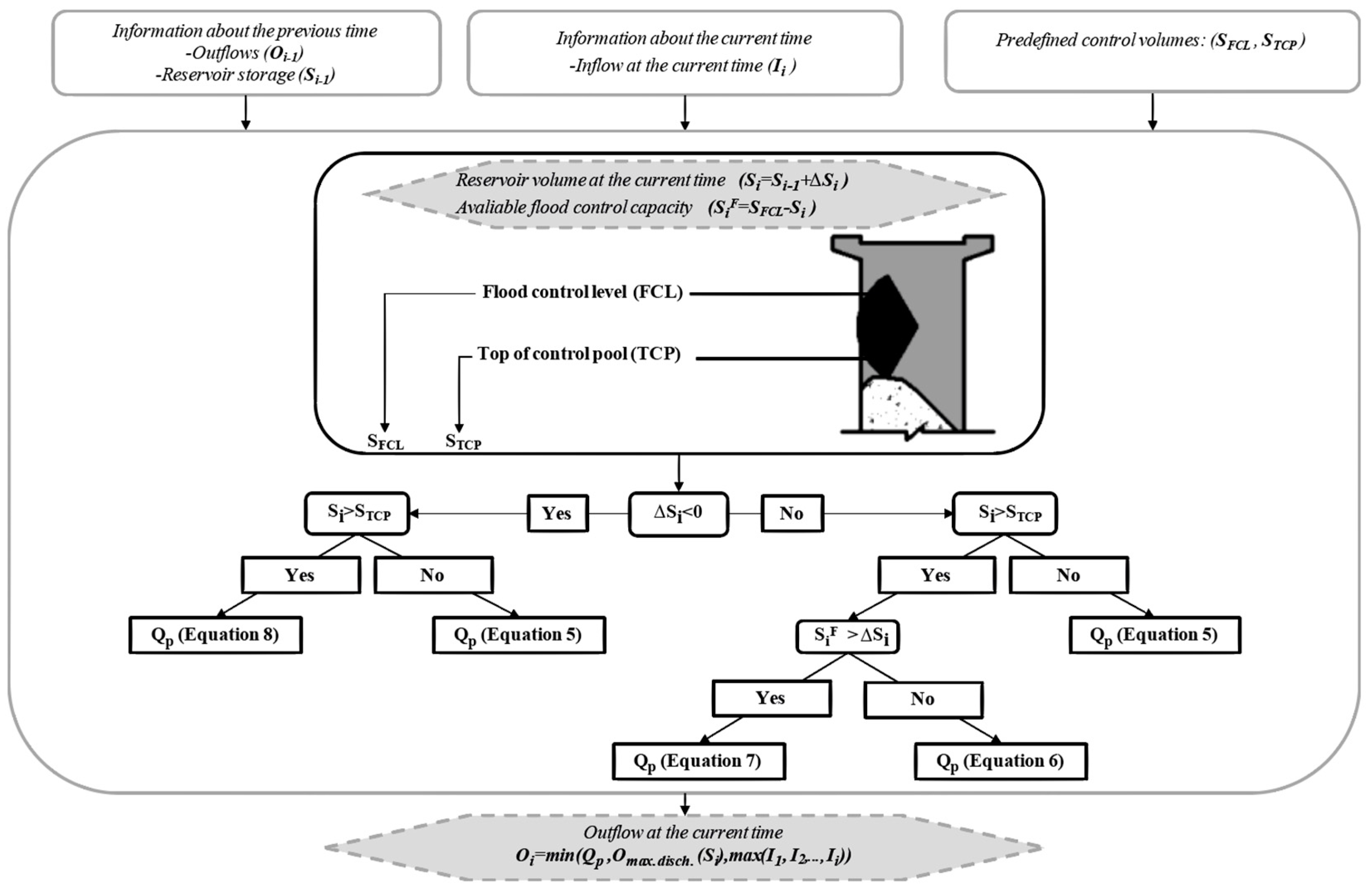
Figure 2 shows the general scheme of the method implementation. The top of control pool (TCP, the corresponding volume is S_TCP) is the maximum reservoir level allowed under ordinary operation conditions in the absence of floods and the flood control level (FCL, the corresponding volume is S_FCL) corresponds to the maximum water level allowed in the reservoir under ordinary operation conditions considering the flood operation [43]. The available flood control capacity at time i $\left({\mathrm{S}}_{\mathrm{i}}^{\mathrm{F}}\right)$ is defined by Equation (1):

$${\mathrm{S}}_{\mathrm{i}}^{\mathrm{F}}={\mathrm{S}}_{\mathrm{FCL}}-{\mathrm{S}}_{\mathrm{i}},$$

(1)

where S_i is the volume in the reservoir at time i.

The VEM progressively manages the available ${\mathrm{S}}_{\mathrm{i}}^{\mathrm{F}}$, increasing the outflows as the ${\mathrm{S}}_{\mathrm{i}}^{\mathrm{F}}$ decreases. Given the reservoir inflow at time i (${\mathrm{I}}_{\mathrm{i}}$), and by assuming a constant inflow in the future, the number of intervals left (n) until the reservoir runs out of ${\mathrm{S}}_{\mathrm{i}}^{\mathrm{F}}$ are given by Equation (2):

$$\mathrm{n}=\frac{{\mathrm{S}}_{\mathrm{i}}^{\mathrm{F}}}{\left({\mathrm{I}}_{\mathrm{i}}-{\mathrm{O}}_{\mathrm{i}-1}\right)·∆\mathrm{t}},$$

(2)

where O_i−1 is the outflow at time i − 1 and Δt represents the operation time step. In this study, we adopted a time step of one hour. Considering that outflows must be equal to inflows when ${\mathrm{S}}_{\mathrm{i}}^{\mathrm{F}}$ = 0 and that outflows increase linearly until equaling the inflows at time $∆\mathrm{t}·\mathrm{n},$ and by assuming a constant inflow in the future, the increment of outflows ($∆{\mathrm{O}}_{\mathrm{i}}={\mathrm{O}}_{\mathrm{i}}-{\mathrm{O}}_{\mathrm{i}-1})$ at each time step is $\frac{\left({\mathrm{I}}_{\mathrm{i}}-{\mathrm{O}}_{\mathrm{i}-1}\right)}{\mathrm{n}}$, and can be expressed by Equation (3) (replacing n by Equation (2)):

$$∆{\mathrm{O}}_{\mathrm{i}}=\frac{\left({\mathrm{I}}_{\mathrm{i}}-{\mathrm{O}}_{\mathrm{i}-1}\right)}{\mathrm{n}}=\frac{{\left({\mathrm{I}}_{\mathrm{i}}-{\mathrm{O}}_{\mathrm{i}-1}\right)}^2·∆\mathrm{t}}{{\mathrm{S}}_{\mathrm{i}}^{\mathrm{F}}}=\frac{∆{\mathrm{S}}_{\mathrm{i}}{}^2}{{\mathrm{S}}_{\mathrm{i}}^{\mathrm{F}}·∆\mathrm{t}},$$

(3)

Equation (3) is valid when the time intervals (n) until the reservoir runs out of flood control capacity are higher than one (${\mathrm{S}}_{\mathrm{i}}^{\mathrm{F}}>∆{\mathrm{S}}_{\mathrm{i}}$). When n ≤ 1, the method aims to balance the outflows and the inflows. When ${\mathrm{S}}_{\mathrm{i}}^{\mathrm{F}}$ = 0, the gates are in operation, maintaining the reservoir level at FCL until they are fully open. Although both antecedent assumptions are not real, by selecting a short time operation step and by recalculating the decision process at each time step, possible deviations are minimized. $∆{\mathrm{O}}_{\mathrm{i}}$ can be expressed as:

$$∆{\mathrm{O}}_{\mathrm{i}}={\mathrm{I}}_{\mathrm{i}}-{\mathrm{O}}_{\mathrm{i}-1}.$$

(4)

The proposed outflow (Q_p) is determined, taking into account S_i and whether the reservoir volume is increasing (ΔS_i = S_i − S_i−1 ≥ 0) or decreasing (ΔS_i < 0) (Figure 2). The different outflows are proposed as follows:

• If S_i $\le$ S_TCP, the method aims to increase the reservoir level to reach the maximum normal operative level (TCP):

  $${\mathrm{Q}}_{\mathrm{p}}=0.$$

  (5)
• When S_i > S_TCP, the outflow proposed depends on ΔS_i:

If ΔS_i ≥ 0, the method releases outflows according to the ΔO previously defined by VEM, as follows:

○

If ${\mathrm{S}}_{\mathrm{i}}^{\mathrm{F}}\le ∆{\mathrm{S}}_{\mathrm{i}}$, the time intervals (n) until the reservoir runs out of flood control capacity are equal to or lower than one, and the method aims to balance the outflows and inflows:

$${\mathrm{Q}}_{\mathrm{p}}={\mathrm{O}}_{\mathrm{i}-1}+\frac{∆{\mathrm{S}}_{\mathrm{i}}}{∆\mathrm{t}}.$$

(6)

○

On the other hand, if ${\mathrm{S}}_{\mathrm{i}}^{\mathrm{F}}>∆{\mathrm{S}}_{\mathrm{i}}$, the VEM progressively manages the available ${\mathrm{S}}_{\mathrm{i}}^{\mathrm{F}}$, increasing the outflows as the ${\mathrm{S}}_{\mathrm{i}}^{\mathrm{F}}$ decreases:

$${\mathrm{Q}}_{\mathrm{p}}={\mathrm{O}}_{\mathrm{i}-1}+\frac{∆{\mathrm{S}}_{\mathrm{i}}{}^2}{{\mathrm{S}}_{\mathrm{i}}^{\mathrm{F}}·∆\mathrm{t}}.$$

(7)

If ΔS_i < 0 (and S_i > S_TCP), the VEM aims to continue decreasing the reservoir level until reaching the TCP:

$${\mathrm{Q}}_{\mathrm{p}}={\mathrm{O}}_{\mathrm{i}-1}+0.5·\left({\mathrm{I}}_{\mathrm{i}}-{\mathrm{I}}_{\mathrm{i}-1}\right).$$

(8)

Once Q_p is obtained, it is compared to the maximum discharge capacity at the current reservoir level (O_max.disch.(S_i)) and the maximum of the antecedent inflows (I₁, I₂, …, I_i), and the minimum of the three values is the flow selected to be released through the gates (O_i).

2.2. The Proposed K-Method

The main advantage of the VEM is its simplicity. It has been widely used in Spain to specify dam management rules for flood control, with successful results. However, it is a fixed method, in the sense that it cannot be adapted to the specific conditions of the basin, the reservoir, or the spillway, other than the flood control volume. The K-Method, based on the VEM [11], proposes the application of a corrective parameter K to the expressions that govern the dam operation rules while the reservoir level is rising. By varying parameter K, we change the proportion in which the outflows are increased, until the FCL is reached. In addition, several improvements to the VEM are included, considering: (1) more reservoir zones to avoid abrupt changes of outflows; (2) an alert outflow (O_ALT) as the maximum admissible flow for avoiding downstream damage; and (3) a maximum gate opening/closing gradient (O_max.Gr). 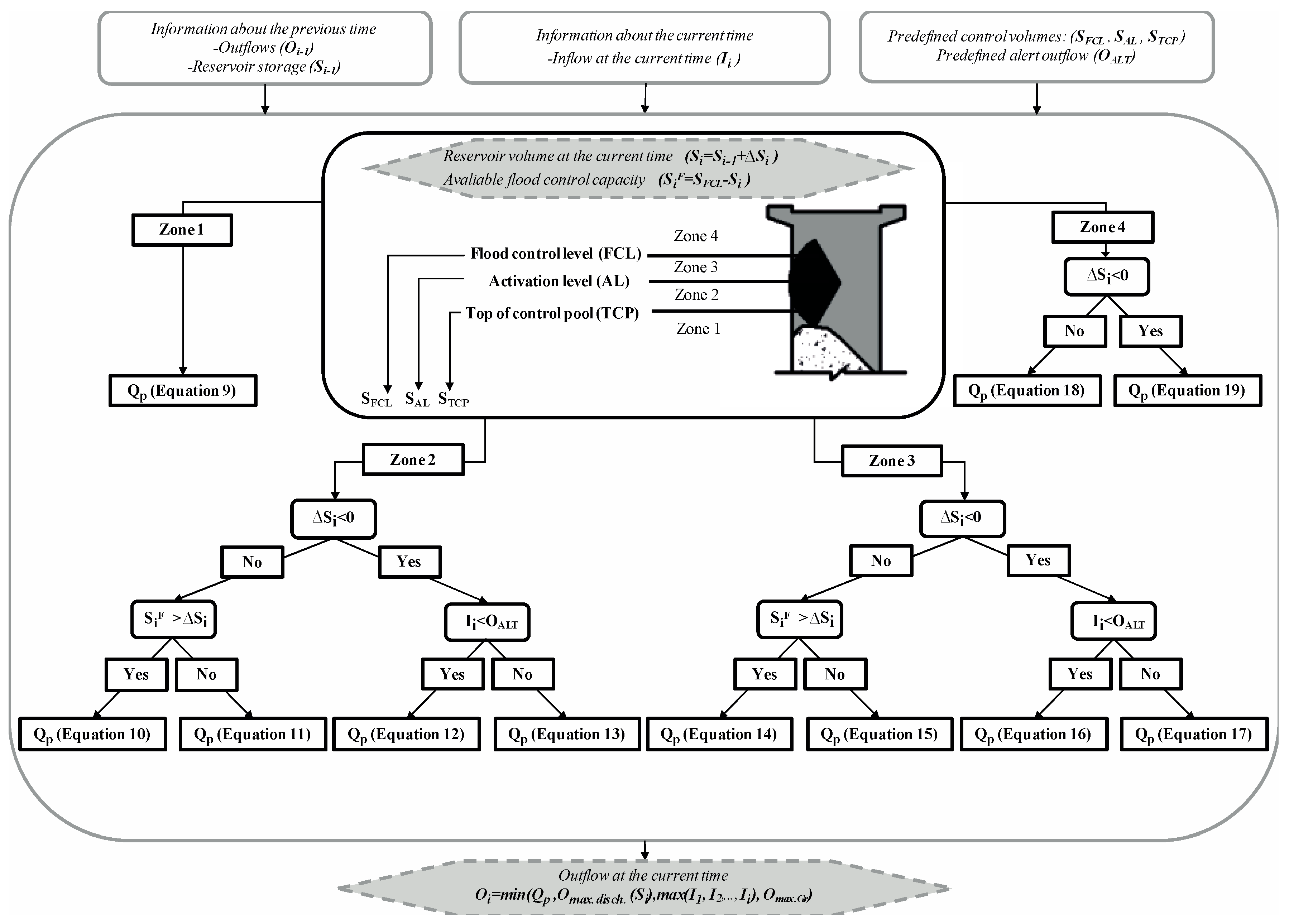Figure 3 shows the general scheme of the K-Method implementation.

The method defines three characteristic levels and reservoir volumes, the aforementioned TCP and FCL, and incorporates the activation level into the scheme (AL, the corresponding volume is S_AL). The activation level is the reservoir level in which the rules of operation change, increasing the outflows. The aforementioned characteristic levels determine four zones: 1, 2, 3, and 4 (Figure 3). The proposed outflow (Q_p) is determined as a function of S_i, the corresponding zone (1, 2, 3, or 4), and whether the reservoir storage is increasing (ΔS_i = S_i − S_i−1 ≥ 0) or decreasing (ΔS_i < 0).

2.2.1. Proposed Outflow in Zone 1

If the reservoir level is within Zone 1, the method aims to increase the reservoir level to reach the maximum normal operative level (TCP):

$${\mathrm{Q}}_{\mathrm{p}}=0.$$

(9)

2.2.2. Proposed Outflow in Zone 2

If the reservoir level reaches Zone 2 and it is rising (ΔS_i ≥ 0), the method gradually starts to release flow, avoiding abrupt changes of outflows that could be dangerous downstream of the dam. The proposed outflow is as follows:

• If ${\mathrm{S}}_{\mathrm{i}}^{\mathrm{F}}>∆{\mathrm{S}}_{\mathrm{i}}$, releases increase linearly from 0 m³/s (when the reservoir level is equal to TCP) to the proposed outflow in Zone 3 at AL:

  $${\mathrm{Q}}_{\mathrm{p}}=\left({\mathrm{O}}_{\mathrm{i}-1}+\mathrm{K}·\frac{∆{\mathrm{S}}_{\mathrm{i}}{}^2}{{\mathrm{S}}_{\mathrm{i}}^{\mathrm{F}}·∆\mathrm{t}}\right)·\frac{{\mathrm{S}}_{\mathrm{i}}-{\mathrm{S}}_{\mathrm{TCP}}}{{\mathrm{S}}_{\mathrm{AL}}-{\mathrm{S}}_{\mathrm{TCP}}}.$$

  (10)
• If ${\mathrm{S}}_{\mathrm{i}}^{\mathrm{F}}\le ∆{\mathrm{S}}_{\mathrm{i}}$, the method aims to balance the outflows and inflows:

  $${\mathrm{Q}}_{\mathrm{p}}={\mathrm{O}}_{\mathrm{i}-1}+\frac{∆{\mathrm{S}}_{\mathrm{i}}}{∆\mathrm{t}}.$$

  (11)

If the reservoir level is within Zone 2 and falling (ΔS_i < 0), the method aims to continue gradually decreasing the reservoir level, avoiding abrupt changes of outflows and minimizing downstream floods:

• If ${\mathrm{I}}_{\mathrm{i}}<{\mathrm{O}}_{\mathrm{ALT}}$, the method releases the maximum precedent outflow limited by the alert outflow:

  $${\mathrm{Q}}_{\mathrm{p}}=\min \left({\mathrm{O}}_{\mathrm{ALT}},\max \left({\mathrm{O}}_1,{\mathrm{O}}_2,\dots ,{\mathrm{O}}_{\mathrm{i}-1}\right)\right).$$

  (12)
• Otherwise, the method maintains the reservoir level, avoiding an increment of downstream floods:

  $${\mathrm{Q}}_{\mathrm{p}}={\mathrm{I}}_{\mathrm{i}}.$$

  (13)

2.2.3. Proposed Outflow in Zone 3

If the reservoir level is within Zone 3 and rising (ΔS_i ≥ 0):

• If ${\mathrm{S}}_{\mathrm{i}}^{\mathrm{F}}>∆{\mathrm{S}}_{\mathrm{i}}$, the method progressively manages the available ${\mathrm{S}}_{\mathrm{i}}^{\mathrm{F}}$, increasing the outflows as the ${\mathrm{S}}_{\mathrm{i}}^{\mathrm{F}}$ decreases:

  $${\mathrm{Q}}_{\mathrm{p}}={\mathrm{O}}_{\mathrm{i}-1}+\mathrm{K}·\frac{∆{\mathrm{S}}_{\mathrm{i}}{}^2}{{\mathrm{S}}_{\mathrm{i}}^{\mathrm{F}}·∆\mathrm{t}}.$$

  (14)
• Otherwise, if ${\mathrm{S}}_{\mathrm{i}}^{\mathrm{F}}\le ∆{\mathrm{S}}_{\mathrm{i}}$, the method aims to balance the outflows and inflows:

  $${\mathrm{Q}}_{\mathrm{p}}={\mathrm{O}}_{\mathrm{i}-1}+\frac{∆{\mathrm{S}}_{\mathrm{i}}}{∆\mathrm{t}}.$$

  (15)

If the reservoir level is within Zone 3 and falling (ΔS_i < 0), the K-Method decreases the reservoir level at a linear rate, from the maximum antecedent outflow to the outflow proposed at AL (limit of Zones 2 and 3):

• If ${\mathrm{I}}_{\mathrm{i}}<{\mathrm{O}}_{\mathrm{ALT}}$, the method releases more than the maximum precedent outflow limited by the alert outflow:

  $${\mathrm{Q}}_{\mathrm{p}}={\mathrm{Q}}_{\mathrm{Eq}.\left(12\right)}+\left(\max \left({\mathrm{O}}_1,{\mathrm{O}}_2,\dots ,{\mathrm{O}}_{\mathrm{i}-1}\right)-{\mathrm{Q}}_{\mathrm{Eq}.\left(12\right)}\right)·\frac{\left({\mathrm{S}}_{\mathrm{i}}-{\mathrm{S}}_{\mathrm{AL}}\right)}{\left(\max \left({\mathrm{S}}_1,{\mathrm{S}}_2,\dots ,{\mathrm{S}}_{\mathrm{i}-1}\right)\right)-{\mathrm{S}}_{\mathrm{AL}})},$$

  (16)
  ${\mathrm{Q}}_{\mathrm{Eq}.\left(12\right)}$ is the proposed outflow in Equation (12).
• Otherwise, the method decreases the reservoir level, minimizing downstream floods:

  $${\mathrm{Q}}_{\mathrm{p}}={\mathrm{I}}_{\mathrm{i}}+\left(\max \left({\mathrm{O}}_1,{\mathrm{O}}_2,\dots ,{\mathrm{O}}_{\mathrm{i}-1}\right)-{\mathrm{I}}_{\mathrm{i}}\right)·\frac{\left({\mathrm{S}}_{\mathrm{i}}-{\mathrm{S}}_{\mathrm{AL}}\right)}{\left(\max \left({\mathrm{S}}_1,{\mathrm{S}}_2,\dots ,{\mathrm{S}}_{\mathrm{i}-1}\right)\right)-{\mathrm{S}}_{\mathrm{AL}})}.$$

  (17)

2.2.4. Proposed Outflow in Zone 4

If the reservoir level is within Zone 4 and rising (ΔS_i ≥ 0), the gates are operated, maintaining the reservoir level at FCL until they are fully open:

$${\mathrm{Q}}_{\mathrm{p}}={\mathrm{O}}_{\mathrm{i}-1}+\frac{∆{\mathrm{S}}_{\mathrm{i}}}{∆\mathrm{t}}.$$

(18)

Conversely, if the reservoir level is within Zone 4 and falling (ΔS_i < 0), the K-Method aims to decrease the reservoir level as soon as possible. The proposed outflow is the one defined during the last interval:

$${\mathrm{Q}}_{\mathrm{p}}={\mathrm{O}}_{\mathrm{i}-1}.$$

(19)

2.2.5. Determination of the Released Outflow at Each Time Step

Once Q_p is obtained, it is compared to the maximum discharge capacity at the current reservoir level (O_max.disch.(S_i)), the maximum of the previous inflows (I₁, I₂, …, I_i), and the maximum gate opening/closing gradient (O_max.Gr.(Si)), and the minimum of the four values is selected as the flow to be released through the gates (O_i).

2.3. I-O and MILP

Finally, we implemented the I-O and MILP methods as extreme performance cases. The I-O exchanges inflows to the reservoir by discharges, so no attenuation effect of the reservoir is considered while the gates are partially opened. I-O corresponds to the extreme case of VEM, where no control flood volume is considered (TCP = AL = FCL). In this case, only Zones 1 and 4 are operative.

We applied the MILP to obtain optimal operation rules in terms of the maximum outflow and maximum level reached in the reservoir for each flood event. MILP was proposed by Bianucci et al. [18], based on the mixed integer linear programming theory, minimizing an objective cost (penalty) function considering the hydraulic and operational restrictions. This objective function (P) is based on the weighted sum of two penalty functions, the P_s associated with the reservoir volumes (and affecting the dam safety) and the P_o associated with the outflows (and affecting the downstream safety), as shown in Equation (20):

$$\mathrm{P}={\mathrm{w}}_{\mathrm{o}}·{\mathrm{P}}_{\mathrm{o}}+{\mathrm{w}}_{\mathrm{s}}·{\mathrm{P}}_{\mathrm{s}},$$

(20)

where w_o and w_s represent the weight associated with P_o and P_s respectively. The reader may refer to Bianucci et al. [18] for a detailed description of the MILP model. It should be stressed that, unlike the three other methods, the MILP method requires knowledge in advance of the entire inflow hydrographs, and therefore, it corresponds to an unrealistic situation.

2.4. Rainfall Generation, Hydrometeorological Model and Comparison of Methods

To compare the behaviour of the different reservoir operation rules during a large range of floods, we considered return periods (Trs) ranging from one to 10,000 years. We generated and analysed 100,000 maximum annual reservoir inflow hydrographs [44,45,46,47], in order to obtain representative and robust results. A semi-distributed event-based hydrometeorological model was applied, based on the Monte Carlo simulation framework proposed by Sordo-Ward et al. [47]. The model stochastically generated a set of probability of exceedance values and their corresponding return periods. By applying an extremal distribution SQRT-Et max [48,49] function, intensity-duration-frequency curves (IDF) [50], and a stochastic rainfall temporal distribution [47], a set of hyetographs was generated. Afterwards, the set of storm events were transformed into hydrographs by applying the Curve Number method [51], the Soil Conservation Service dimensionless unit hydrograph procedure [51], and the Muskingum method [52]. The reader may refer to Sordo-Ward et al. [47] for a more detailed description of the processes involved.

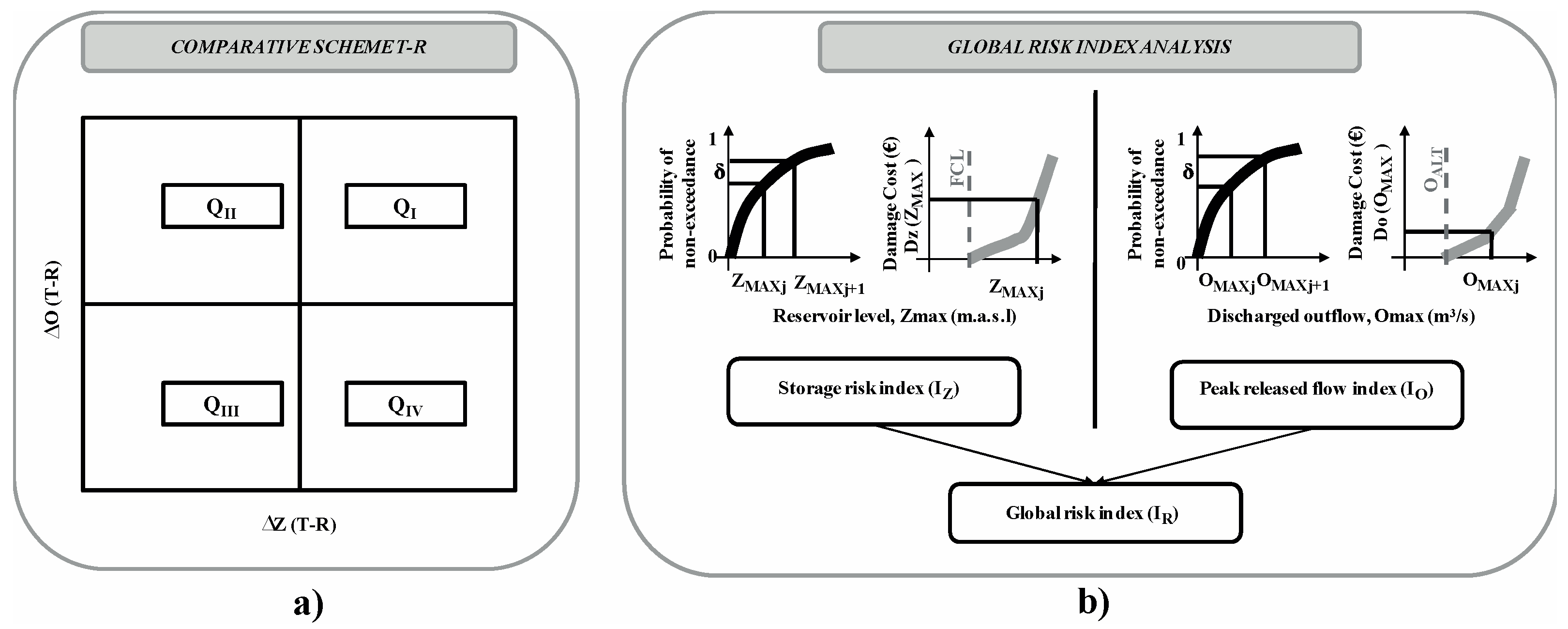
Once the different gate controlled operation rules were applied, we selected the maximum level reached in the reservoir (Z_MAX) and the maximum outflow downstream (O_MAX) as representative variables for a comparison of the methods’ performance. We implemented a comparative analysis by means of two different approaches (Figure 4). On the one hand, we applied a comparative scheme organized in quadrants, which showed the increasing (or decreasing) of the maximum reservoir level and maximum outflow compared to the VEM (Figure 4a). The points located in the upper right quadrant (Q_I) represent events where the maximum level reached in the reservoir and the maximum outflow were higher than by applying the VEM. The points located in the upper left quadrant (Q_II) show an intermediate situation, with lower maximum levels but higher outflows. The lower left quadrant (Q_III) represents cases for which both the maximum level and maximum outflow were lower than by applying the VEM (i.e., the best situation). The lower right quadrant (Q_IV) represents intermediate situations with higher maximum levels and lower maximum outflows. On the other hand, we implemented the global risk index (I_R) analysis (Figure 4b) proposed by Bianucci et al. [18]. This method accounts for a single indicator of the global risk associated for the Z_MAX and O_MAX, by applying the concept of expected annual damage [53]. First, the damage cost curves (D_Z and D_O) and the cumulative distribution functions (CDF) related to Z_MAX and O_MAX were obtained, based on the information included in the Dam Master Plan and the Dam Emergency Plan. The global risk index is obtained by multiplying the probability of the reference variable (Z_MAX or O_MAX) in the given interval by the damages associated with that variable’s value. In the case of O_MAX, the damages are calculated through floodplain analysis. In the case of Z_MAX, the damages are estimated as the product of the probability of reaching during the flood, provided that the reservoir has already reached Z_MAX, multiplied by the damages linked to dam failure. It is important to point out that there was no expected damage below FCL and O_ALT (Figure 4b). Afterwards, we obtained the partial risk indexes I_Z (Equation (21)) and I_O (Equation (22)) associated with Z_MAX and O_MAX, respectively:

$${\mathrm{I}}_{\mathrm{Z}}=\mathsf{\delta }·{{\displaystyle \sum }}_{\mathrm{j}=1}^{\mathrm{n}-1}\left(\mathrm{Dz}\left(\frac{{\mathrm{Zmax}}_{\mathrm{j}}+{\mathrm{Zmax}}_{\mathrm{j}+1}}{2}\right)\right),$$

(21)

$${\mathrm{I}}_{\mathrm{O}}=\mathsf{\delta }·{{\displaystyle \sum }}_{\mathrm{j}=1}^{\mathrm{n}-1}\left(\mathrm{Do}\left(\frac{{\mathrm{Omax}}_{\mathrm{j}}+{\mathrm{Omax}}_{\mathrm{j}+1}}{2}\right)\right),$$

(22)

where D_Z and D_O are the damage functions for Z_MAX and O_MAX, respectively, and $\mathsf{\delta }$ represents the incremental non-exceedance probability between two consecutive elements in the sample (either O_MAX or Z_MAX (Figure 4b)), being constant and equal to the inverse of the size of the generated sample (100,000 in the current study). The index j represents the position of the sorted series (ascending order) of maximum outflows and maximum reservoir levels. Once I_O and I_Z were obtained, we used the weighted sum aggregation to obtain the global risk index (I_R). Due to the lack of information, we designated equal levels of priority to both partial indexes (Equation (23)):

$${\mathrm{I}}_{\mathrm{R}}={\mathrm{I}}_{\mathrm{Z}}+{\mathrm{I}}_{\mathrm{O}},$$

(23)

for which all of the mentioned indexes are expressed in euros.

When comparing the aforementioned methods, it should be highlighted that the VEM, K-Method, and I-O operate in real-time, using only the precedent information. Meanwhile, MILP utilizes, as the input, the entire set of inflow hydrographs. In this study, MILP was applied to obtain the maximum possible improvement in terms of O_MAX and Z_MAX.

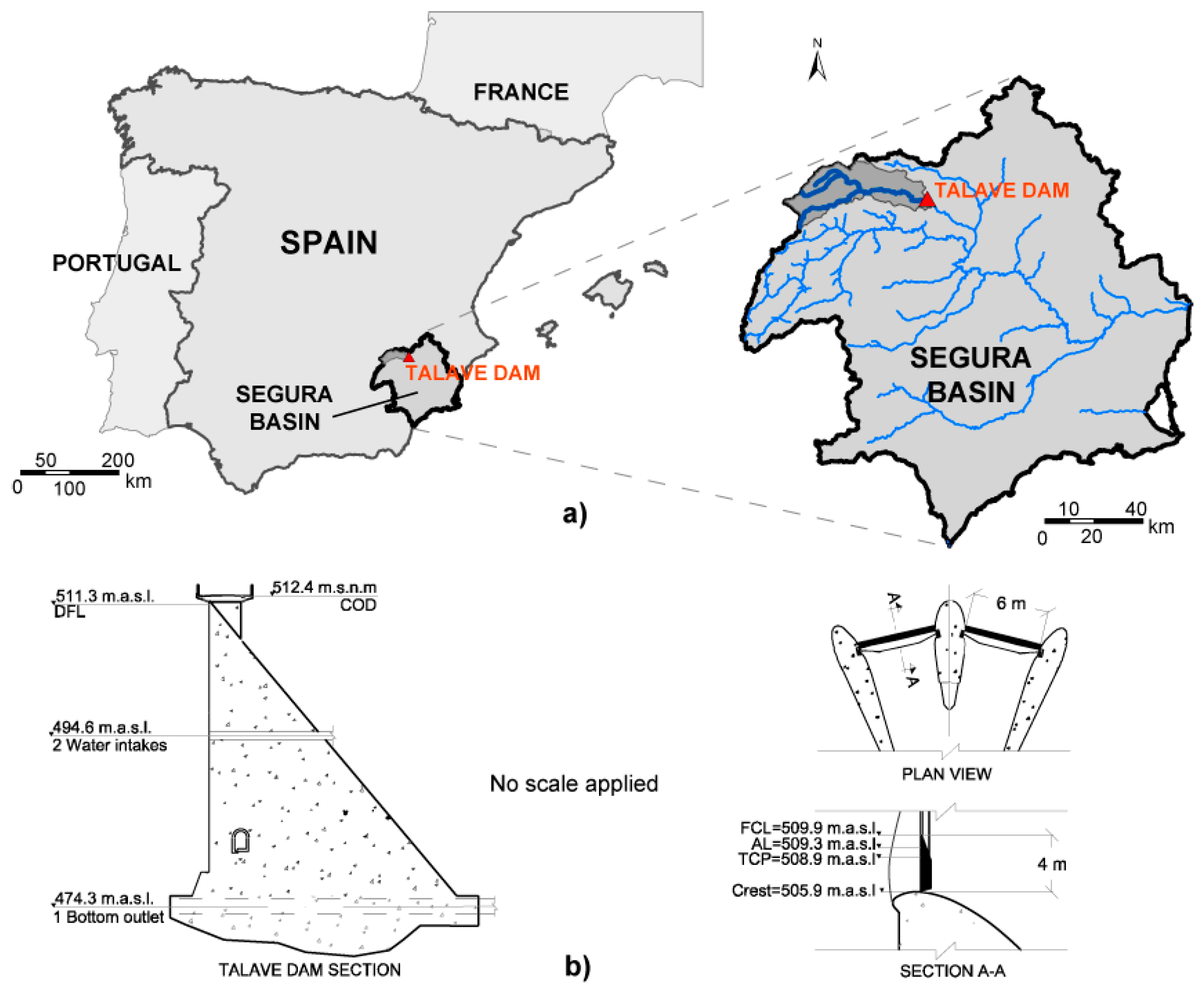
2.5. Case Study

The proposed methodology was applied to the Talave reservoir. It is located in the province of Albacete, in the southeast of Spain, and belongs to the Mundo river basin. The Talave basin has an area of 766.5 km². The climate of the region is Mediterranean (mean annual precipitation of 557 mm). The main purposes of the reservoir are flood regulation, hydropower generation, and water supply for the Region of Murcia.

The characteristics of the basin and dam-reservoir system configuration are shown in Figure 5 and

Table 1. Characteristic reservoir levels and outflows of the dam configuration.

Reservoir Levels (m.a.s.l)		Maximum Outflow Capacity at Design Flood Level (DFL) (m3/s)		Characteristic Outflows (m3/s)
Top of control pool (TCP)	508.9	Gated-spillway	2 × 142.5	Alert outflow (OALT)	100
Activation level (AL)	509.3
Flood control level (FCL)	509.9	Bottom outlet	1 × 99.5	Warning outflow (OWARN)	150
Design flood level (DFL)	511.3	Dam body water intakes	2 × 9.0	Emergency outflow (OEMER)	300
Crest of dam (COD)	512.4

. Two vertical wagon gates, each one being six meters wide by four meters high, compose the main spillway. The other operative discharge structures are one bottom outlet and two water intakes in the dam body.

3. Results and Discussion

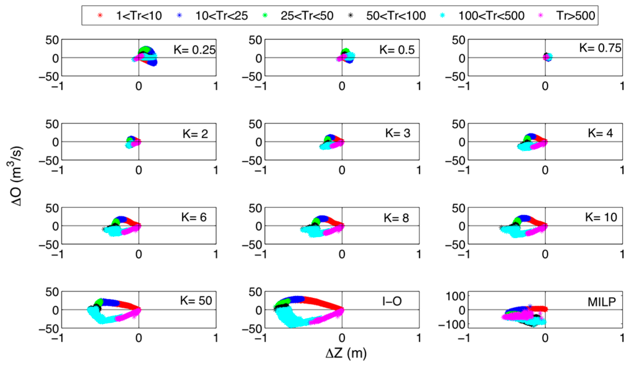
Results comparing a representative range of K-values, I-O, and MILP with the VEM, are reported in Figure 6, Figure 7 and Figure 8. For K-values lower than one, no improvement with respect to the VEM was achieved for the Talave dam. The K-Method is equal to the VEM when the K-value is equal to one. For K-values higher than one, all analysed cases were located in Q_II and Q_III. Following this, we focused the analysis of the K-Method on K-values higher or equal to one. When analysing the variations of the maximum reservoir level compared to VEM (ΔZ), a higher K-value resulted in a lower Z_MAX, regardless of the range of inflow Trs studied, reaching up to −0.15 m for K = 2 and −0.64 m for K = 50 (Figure 6). However, when analysing the variations of the maximum outflows compared to VEM (ΔO), different behaviours were found, depending on the Trs analysed. 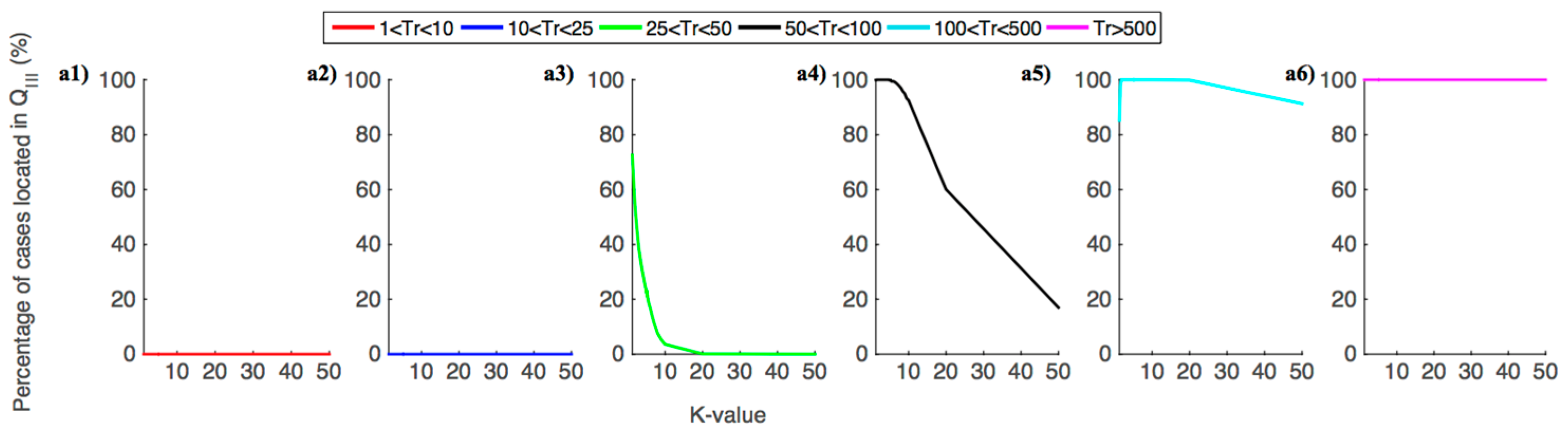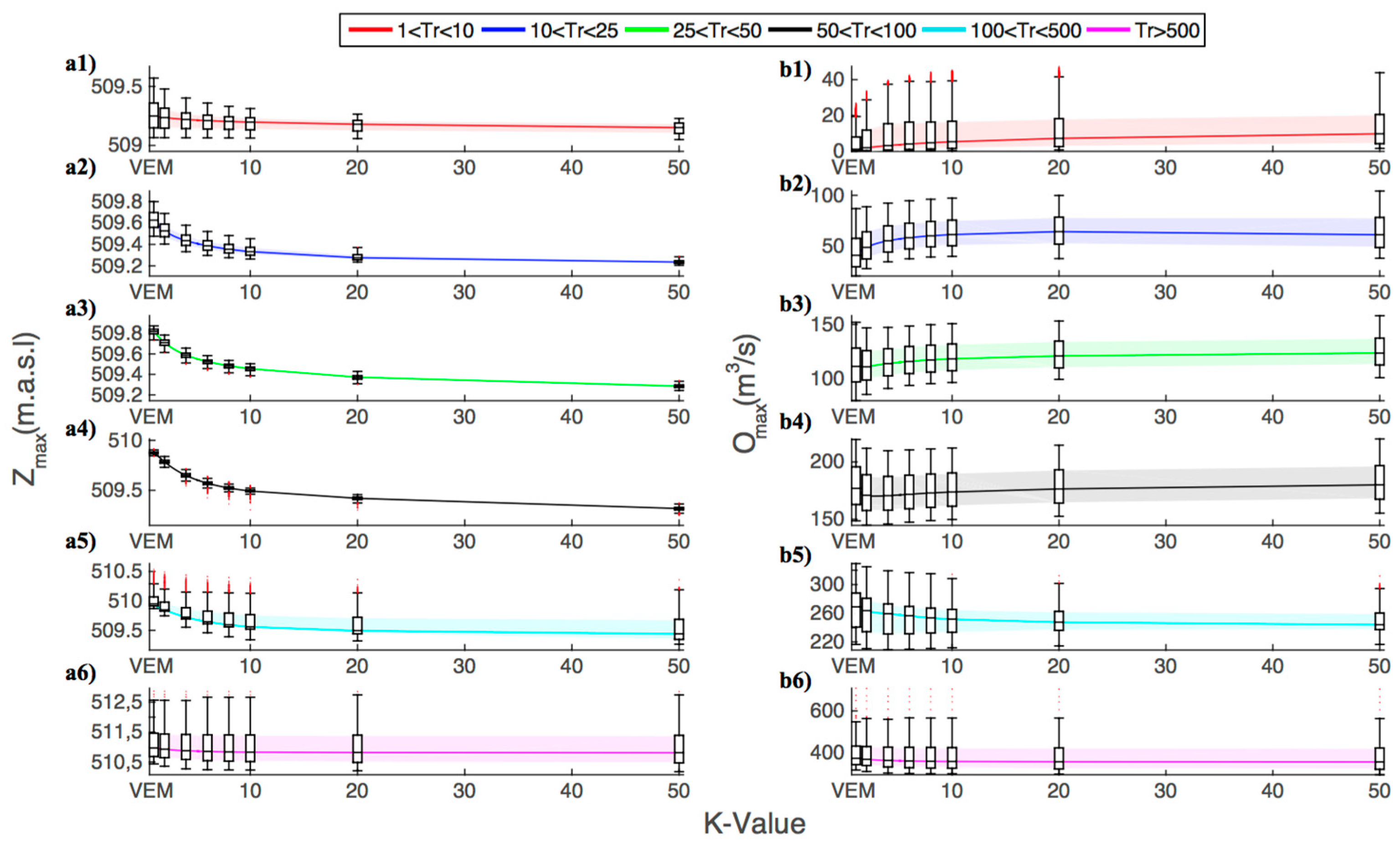Figure 7 shows, for different ranges of Trs, the percentage of cases located in Q_III (the best situation), Figure 8(a1–a6) shows the median and quartiles associated with the maximum reservoir levels (Z_MAX), and Figure 8(b1–b6) shows the variations of the median and quartiles associated with the maximum outflows (O_MAX).

For Tr values lower than 25 years, all events were located in Q_II, regardless of the analysed K-value (Figure 7(a1,a2)), decreasing the maximum levels but increasing the maximum outflows when compared with VEM (Figure 6 and Figure 8(a1,a2,b1,b2). Even though the maximum outflows increased, the O_MAX values did not jeopardize the downstream safety for K-values lower than ten, because O_ALT was not exceeded (O_MAX = 97.2 m³/s for K = 10).

For Tr values ranging from 25 to 50 years, lower K-values included more cases in Q_III, decreasing from 73% for K = 1.25, to 4% for K = 10. For K-values higher than 20, all events were located in Q_II (Figure 7(a3)). Higher K-values achieved lower Z_MAX values, but the opposite occurred for O_MAX. For example, the Z_MAX median decreased from 509.8 to 509.5 m and the O_MAX median increased from 111 to 118 m³/s for K = 1 (VEM) and K = 10, respectively (Figure 8(a3–b3)). For K-values higher than ten, the median of Z_MAX decreased to 509.3 m for K = 50, while the O_MAX median increased to 124 m³/s for K = 50.

For Tr values ranging from 50 to 100 years, more than 99% of the analysed cases were included in Q_III for K-values from 1.25 to 6.5, more than 92% for K-values lower than ten, and this decreased down to 17% for K = 50 (Figure 7(a4)). The median of Z_MAX decreased from 509.9 m for K = 1 (VEM), to 509.5 m for K = 10 and 509.3 m for K = 50. (Figure 8(a4)). The median of O_MAX decreased from 177 m³/s to 170 m³/s with K ranging from one (VEM) to three, but increased for K-values higher than three, up to 180 m³/s for K = 50 (Figure 8(b4)).

For Tr values within the range of 100 to 500 years, all events were located in Q_III for K-values ranging from one to ten (Figure 6 and Figure 7(a5)) and more than 93% for K-values higher than ten (Figure 7(a5) and Figure 8(a5,b5)). The Z_MAX and O_MAX median values decreased from 510.0 m and 270 m³/s for K = 1 (VEM), to 509.6 m and 252 m³/s for K = 10, respectively. For K-values higher than ten, the Z_MAX and O_MAX median values remained almost constant.

For Tr values higher than 500 years, regardless of the K-value (except for those lower than one), all events were located in Q_III (Figure 6 and Figure 7(a6)). The Z_MAX and O_MAX median values ranged from 511.0 m and 375 m³/s for K = 1 (VEM), to 510.8 m and 360 m³/s for K = 10, respectively (Figure 8(a6,b6)). For K-values higher than ten, the Z_MAX and O_MAX median values remained almost constant. We also compared I-O and MILP with VEM. As expected, the I-O behaviour was similar to the K-Method for higher K-values (Figure 6). By comparing MILP and VEM, the results showed that all events with a Tr higher than 25 years were located in Q_III, and those with a Tr lower than 25 years located in Q_II presented outflows that did not jeopardize the downstream safety (Figure 6).

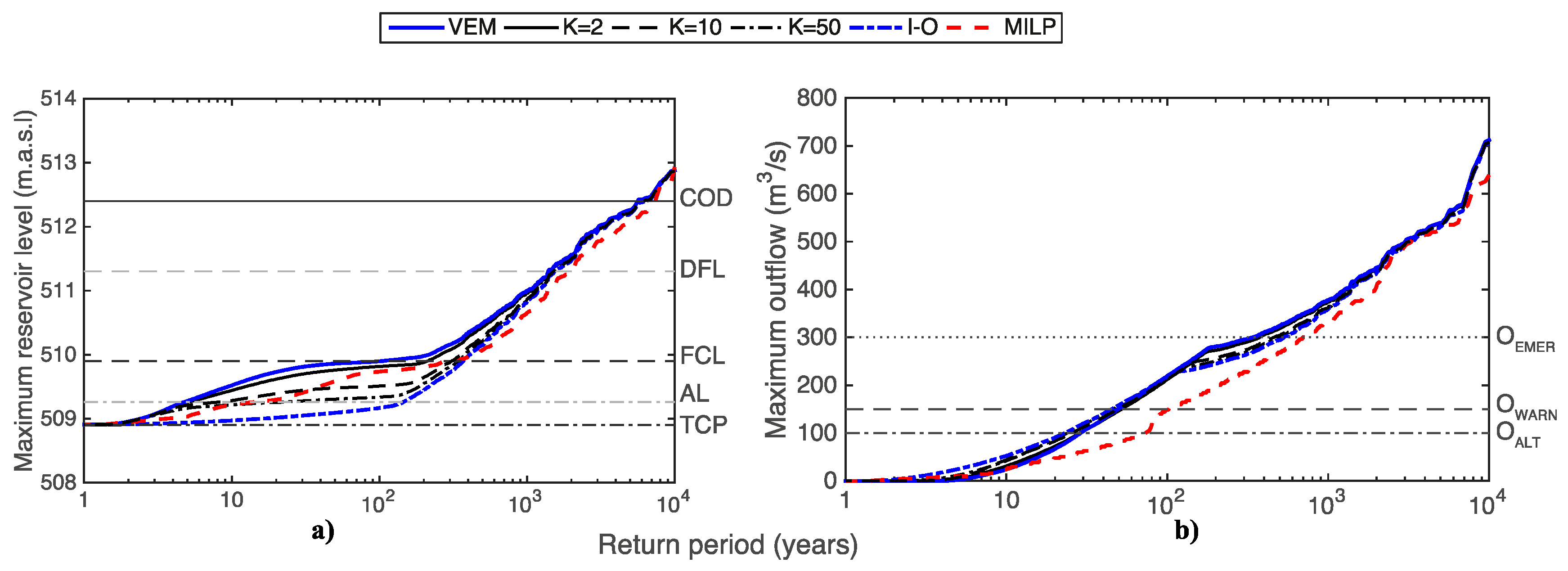
Finally, we analysed the frequency curves of Z_MAX and O_MAX for the different methods (Figure 9). For the K-values analysed (and for K-values greater than one), they showed an intermediate behaviour between VEM and I-O. For the Z_MAX frequency curves, the higher the K-value, the lower Z_MAX obtained for the same return period (Figure 9a). However, when analysing the O_MAX frequency curves, they intersected the VEM maximum outflow frequency curve (Figure 9b). For Tr values higher than one, and until the intersection of the O_MAX frequency curves, the greater the K-value, the greater the O_MAX was for the same Tr. Moreover, the intersection with VEM occurred at higher Trs, corresponding to a Tr of 31, 50, 86, and 102 years for K = 2, 10, 50, and I-O, respectively. Once the O_MAX frequency curves intersected, the behaviour was the opposite.

Therefore, the choice of the best operation rule was not univocal for the entire range of analysed Tr and depended on the priorities selected by the dam damager (MILP was not accounted for as it needs to know the whole inflow hydrograph in advance). If an ordinary reservoir operation and the management of floods with a Tr between one and 25 years were prioritized, the best rule operation was the K-Method for the highest K-value that minimized Z_MAX and avoided damages associated with the released outflows. As mentioned, for this case study, it was K = 10.

If the management of floods with a Tr ranging from 25 to 500 years was prioritized, the best operation rule depended on whether the number of events included in Q_III or the entity of the decrease of Z_MAX and O_MAX was prioritized. In the case study, K = 1.25 maximized the number of events improved for 25 < Tr < 50 years and K = 10 for 50 < Tr < 500 years. The reservoir levels reached Zones 3 (in all events with Tr values higher than 50 years) and 4. The influence of the K-value on Equation (10) implied an increase of the released outflows at the beginning of the operation (Zone 2), increasing the available flood control capacity with respect to VEM for the next time steps. Therefore, Zones 3 and 4 were reached later, for which the O_MAX was reduced (Figure 3).

If the dam safety and management of extreme floods (Tr > 500 years) were prioritized, I-O simultaneously minimized the maximum levels and maximum outflows. However, as the Tr of the inflows increased, ΔO and ΔZ tended to be zero. In these cases, Q_p was higher than the maximum discharge capacity when the gates were fully opened and the outflow responded to an un-controlled fixed-crested spillway (Figure 3). This explains why Z_MAX and O_MAX tended to be constant when analysing K-values higher than ten for Tr values higher than 500 years (Figure 8(b6) and Figure 9). This also explains the shape of the half loop of the comparative scheme between the K-Method and VEM (Figure 6).

In a practical case, even if the skill required to forecast the inflow hydrograph is limited, there may be ways to identify the entity of the flood that is being managed in the reservoir. According to the general meteorological situation, the dam manager may be able to estimate the return period of the event that is occurring, and therefore, the conclusions of the above discussion could be applied to decide on the best K-value to adopt.

Finally, Figure 9 shows changes in the slope for both the Z_MAX and O_MAX frequency curves, and regardless of the analyzed operation rule. For small and medium floods, the outflows are governed by the operation of the partially opened gates. Once the FCL is exceeded and gates become fully open, the spillways work as un-controlled fixed-crested spillways, justifying the behavior of the frequency curves.

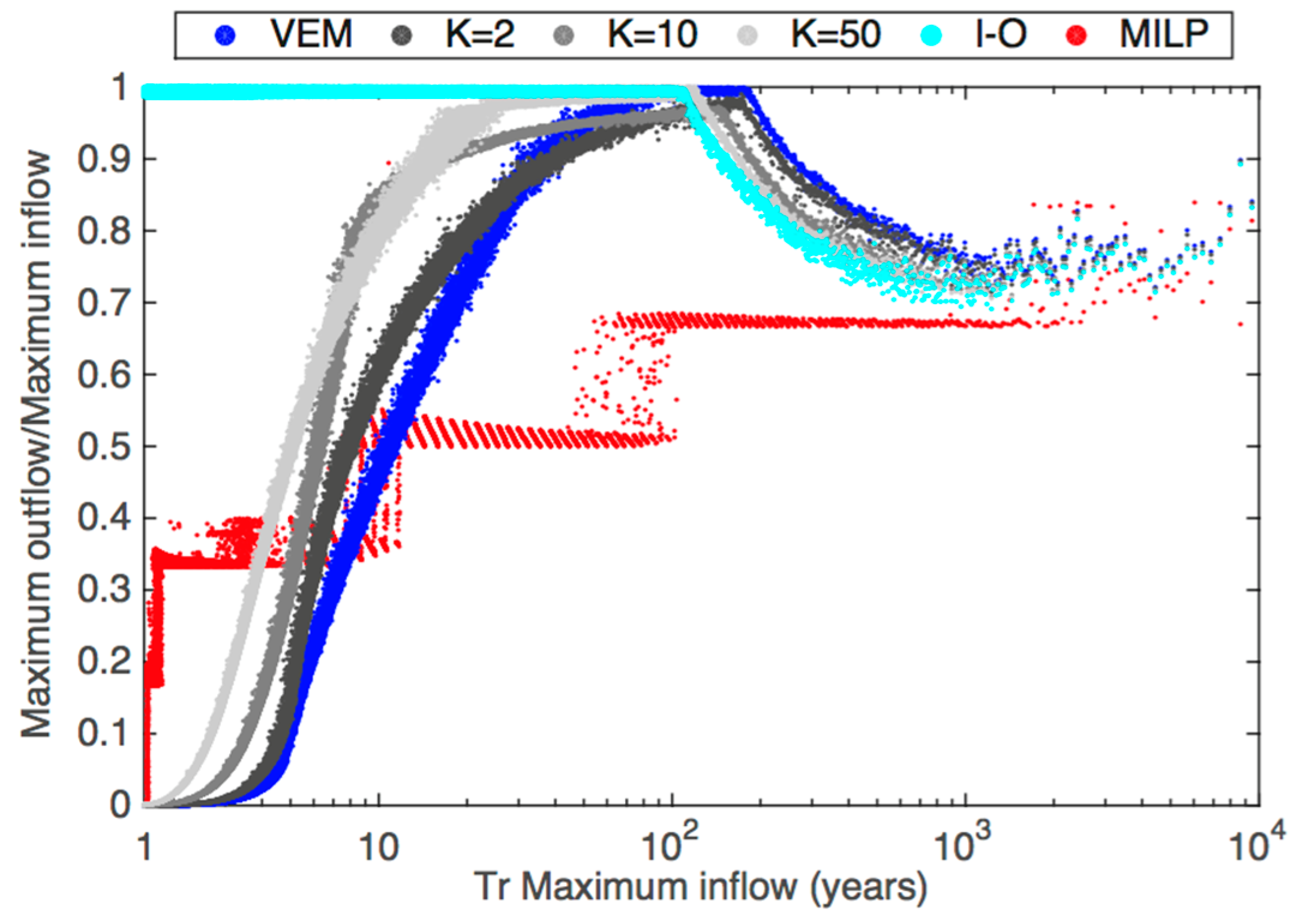
Figure 10 shows the evolution of the ratio between the maximum outflow and the maximum inflow as a function of the return period of each event for different dam operation methods. Although MILP showed the most peak attenuation, as previously stated, it represents perfect management under the unrealistic assumption of full knowledge of the inflow hydrograph; thus, it was taken only as the reference for maximum improvement. Regarding the behaviors of the real-time methods, we distinguished three main phases. For a lower Tr, when all methods were active (gates partially opened), the VEM was the real-time method which showed the highest peak attenuation, because the other real-time methods specify greater outflows than those of VEM. In addition, the other methods reached the fully opened gate situation earlier than VEM, because they released greater outflows and the spillways started to work earlier as un-controlled fixed-crested spillways. For medium and high Tr values, the mentioned change in the release mechanism justifies an increase of peak attenuation and the differences among the methods decrease. Finally, for the biggest floods where the crest of the dam is overtopped and the entire length of the dam works as an un-controlled fixed-crested spillway, peak attenuation decreased, regardless of the method.

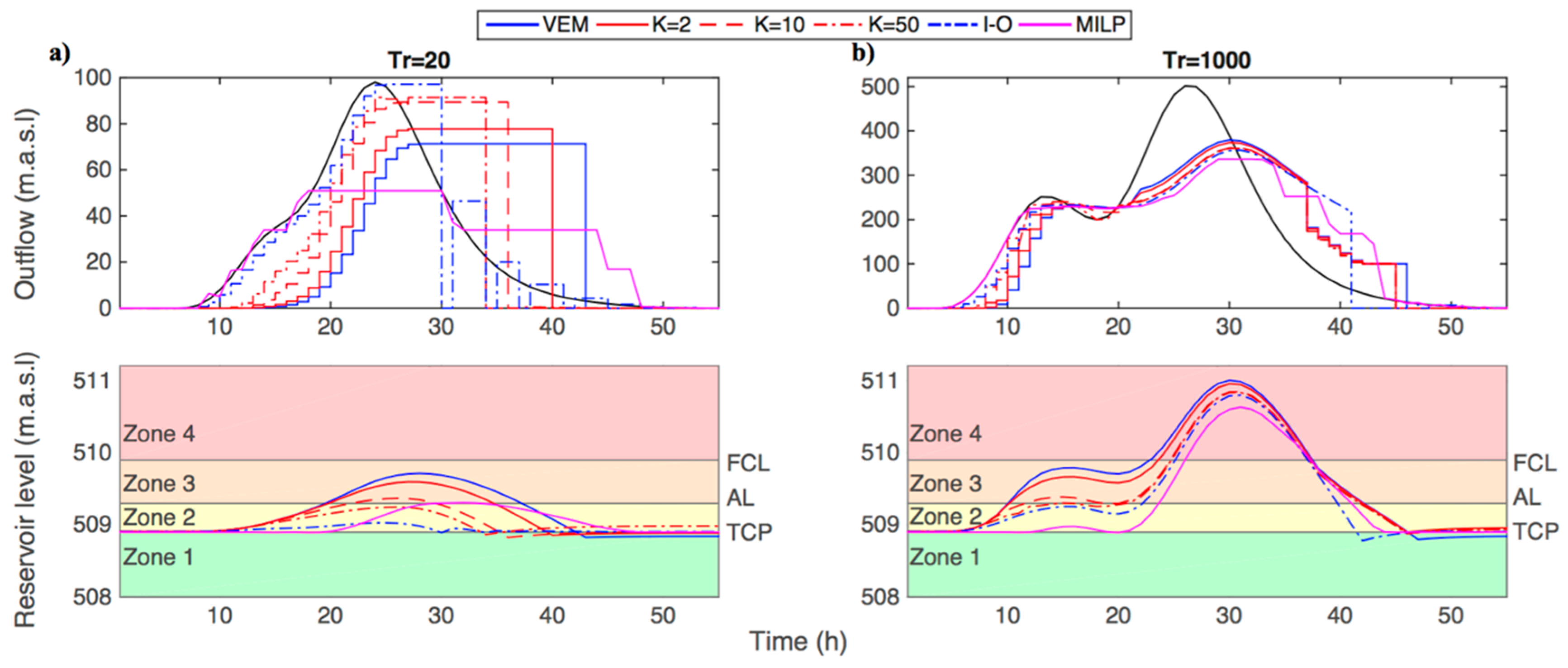
Figure 11 shows two examples of application of the different proposed dam operation methods. Although MILP showed the most attenuation of peak flows for both cases and good behaviour regarding the maximum reservoir level, it represents perfect management under the unrealistic assumption of full knowledge of the inflow hydrograph. Therefore, it was only taken as the reference for maximum improvement. For a moderate flood, Figure 11a shows considerable differences of maximum peak flows and maximum reservoir levels, and the VEM was the real-time method which presented the highest peak attenuation, but the highest maximum reservoir level. In the analysis of a large flood (Tr = 1000 years, Figure 11b), it can be seen that the gates became fully open (around 20 h) for all methods. From this time on, the spillways start to work as un-controlled fixed-crested spillways. The peak attenuation effect is mainly due to the un-controlled fixed-crested spillway mechanism and the differences among the methods decrease.

In order to better quantify the influence of the K-value, we applied a risk-based analysis. Once we obtained the damage curves (Figure 12a,b), we calculated the storage risk index (I_Z), the peak released flow index (I_O), and the global risk index (I_R) for the Talave dam (Figure 12c).

Figure 12 shows that K-values larger than one reduce the I_R value for the Talave dam with respect to the VEM. There is also a range of K-values for which the I_R is even lower than for the I-O, which is a very conservative flood management strategy. This global reduction is due to the effect of management strategies on the I_O. If I_O is analysed, I-O is found to be the worst strategy, since it implies no peak attenuation during the controlled phase of the flood. The K-Method outperforms the VEM for K-values smaller than 20. For the case of the I_Z, the minimum values are obtained for the I-O strategy, which emphasizes controlling the reservoir level. This strategy is even better than MILP optimization. In the case of the K-Method, it always outperforms VEM, and I_Z tends to be the value obtained for I-O for large values of K. MILP represented the minimum expected value for I_R. For this case study, the K-value that optimized I_R is 5.25, reducing the annual expected damage by 8.4%, when compared to VEM. The reduction represented 17.3% of the maximum possible reduction determined by MILP. Even though this may seem like a small reduction, it should be taken into account that the application of the K-Method has no associated construction costs and the improvement would be applied annually, during the whole dam life (according to the Dam Master Plan, Talave Dam’s expected life is 167 years).

4. Conclusions

The proposed K-Method is a decision-making tool for dam managers that allows analyzing the effects of applying different reservoir operation rules for both dam safety and downstream safety. In contrast with other fixed methods, the K-Method allows, for each analyzed dam, the identification of the K-value (conducting a calibration process) that best adapts the management strategy to the specific conditions of the basin, the reservoir, the spillway, and to the objectives of flood management. It should be noted that the proposed method has been applied to only one basin and dam configuration, which limits the generalization of the results and conclusions obtained. Although the results are promising, further research should be developed to ensure that the K-method improves the rules of operation of flood control through a wide range of gated-spillway dams.

For the case study under analysis, the K-Method improved the results obtained with VEM, by reducing the maximum reservoir levels reached in the dam (the higher the K-value. the lower the maximum reservoir level), while the corresponding increase of outflows did not endanger downstream safety. In addition, by carrying out a dam risk analysis, a K-value of 5.25 lowered the global risk index, I_R, by 8.4% compared to VEM, and represented 17.3% of the maximum possible reduction determined by MILP.

We identified different behaviors, depending on the Trs analyzed. For events with a Tr ranging from one to 25 years, K-value = 10 resulted in an important decrease in the maximum reservoir levels, while the corresponding increase of outflows did not endanger downstream safety.

For events with a Tr ranging from 25 to 100 years, higher K-values reduced the number of events that simultaneously achieved lower maximum levels and outflows. For events with a Tr higher than 500 years, I-O simultaneously achieved the lowest maximum levels and outflows. In a practical case, even if the skill required to forecast the inflow hydrograph is limited, according to the general meteorological situation, the dam manager may be able to estimate the return period of the event that is occurring and therefore the conclusions obtained could be applied to decide on the best K-value to adopt.