Simulink Implementation of a Hydrologic Model: A Tank Model Case Study


Abstract
:1. Introduction
2. Materials and Methods
2.1. Simulink Modeling Framework
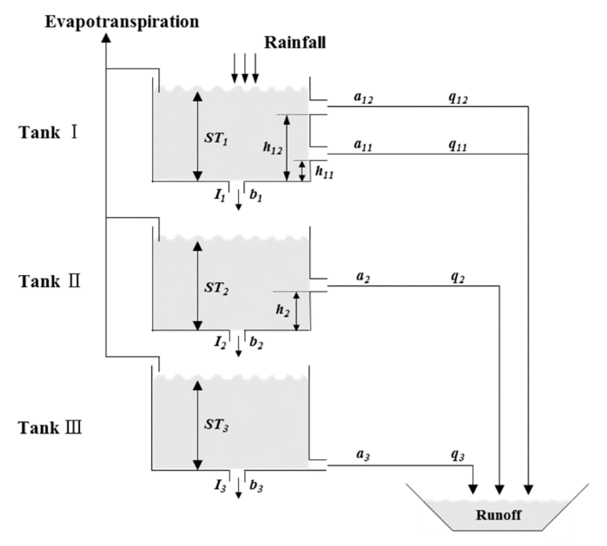
2.2. The Tank Model
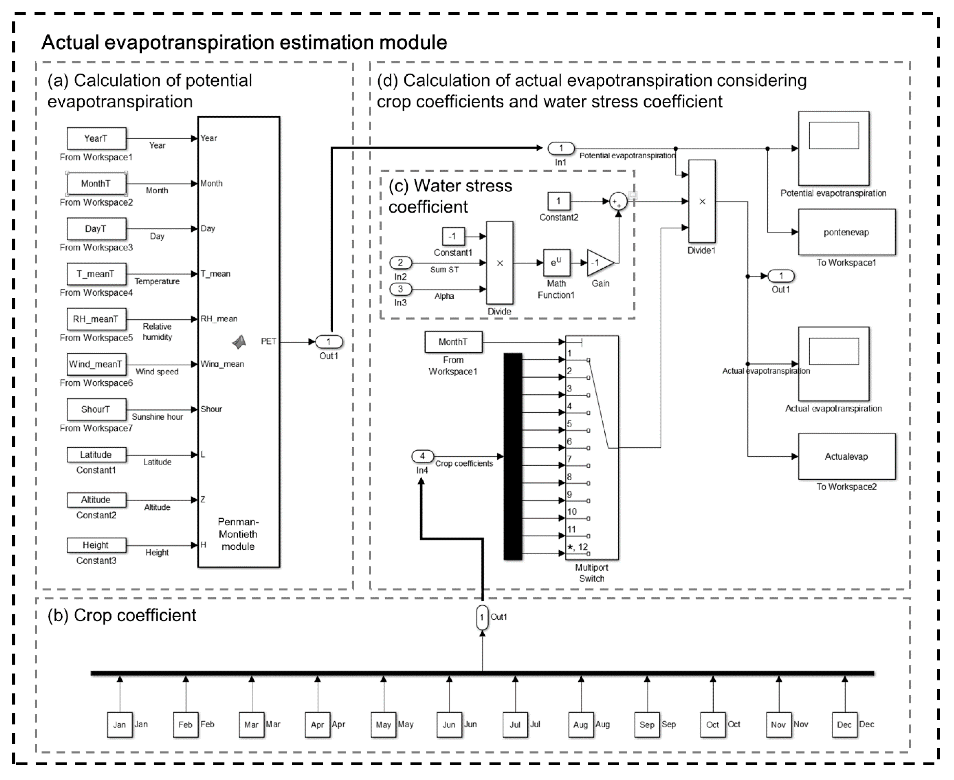
2.3. Watershed Evapotranspiration
2.3.1. Potential Evapotranspiration
2.3.2. Crop Coefficient
2.3.3. Soil Water Stress Coefficient
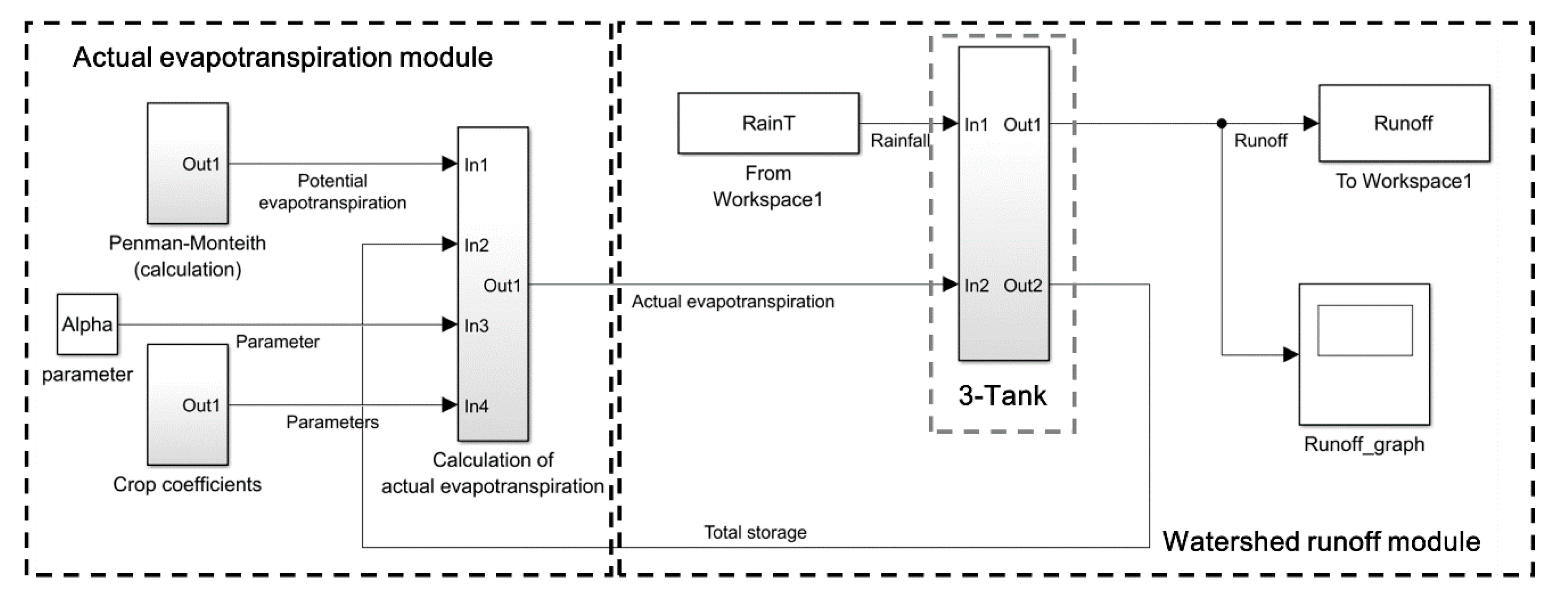
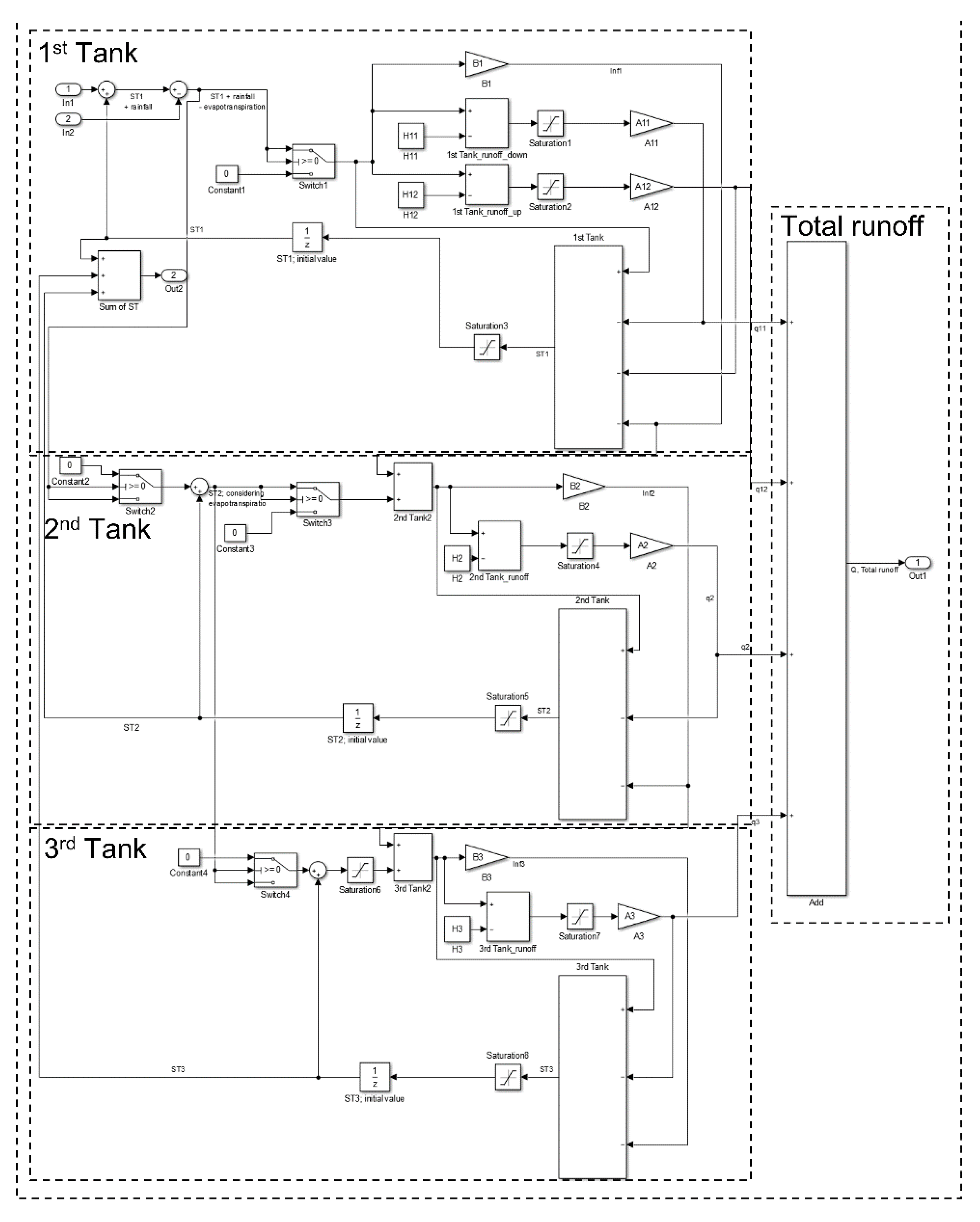
3. Simulink-Tank Model Structure
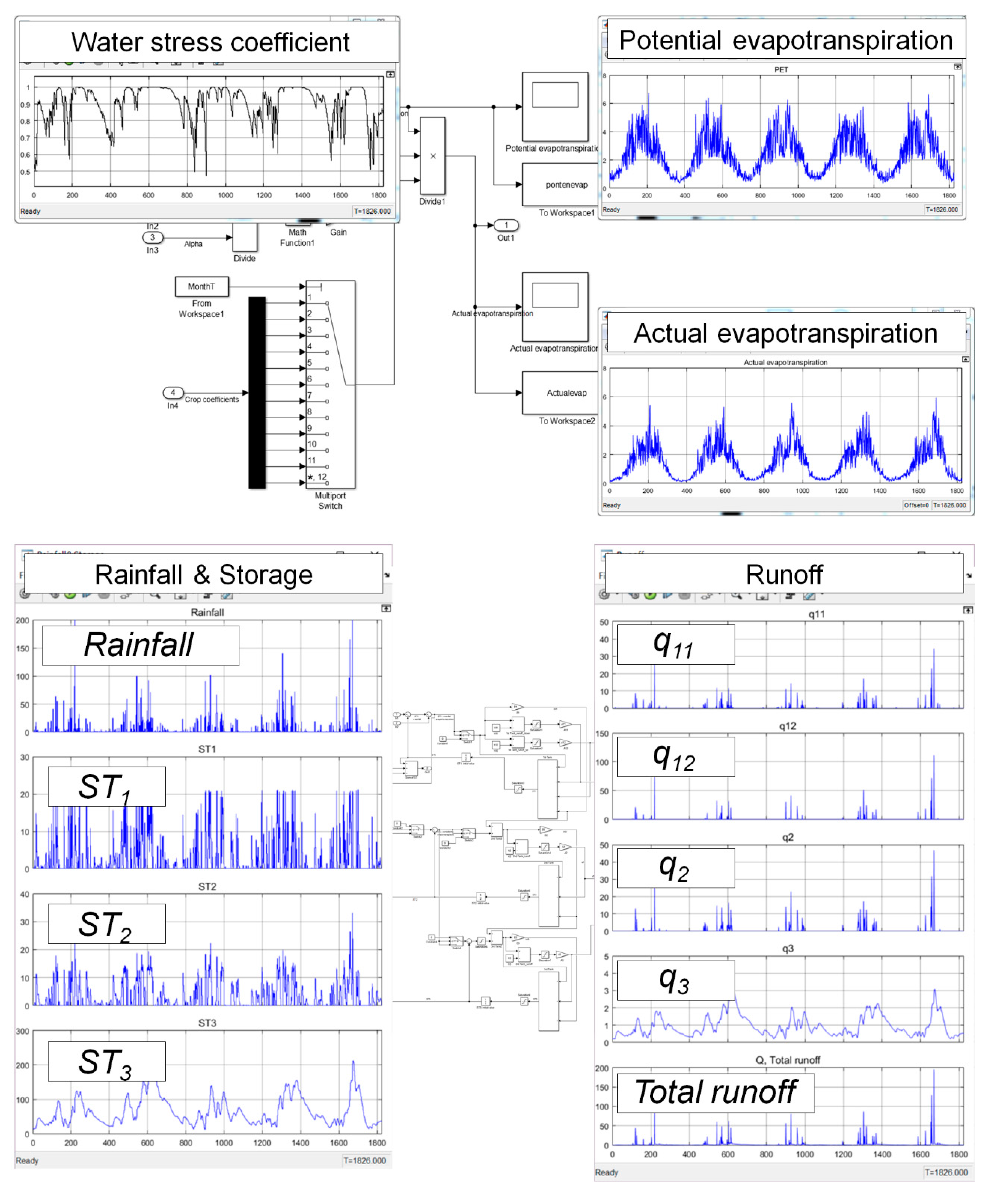
3.1. Watershed Evapotranspiration Module
3.2. 3-Tank Module
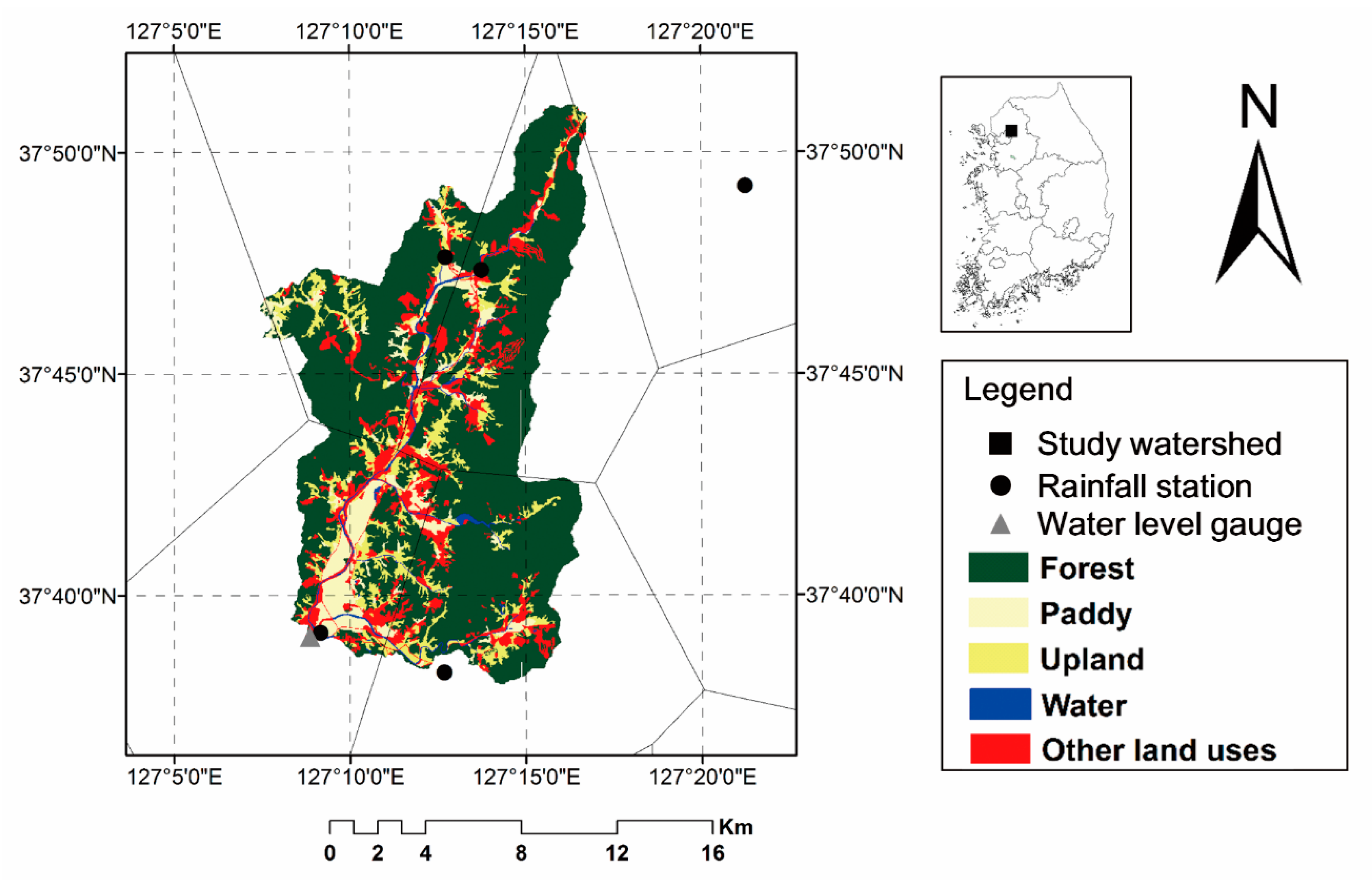
4. Case Study
5. Application and Discussion of the Simulink-Tank Model
5.1. Dynamic Description of a Hydrologic System
5.2. Parameter Calibration for the Simulink-Tank Model Using Optimization Techniques within MATLAB
5.2.1. Objective Function
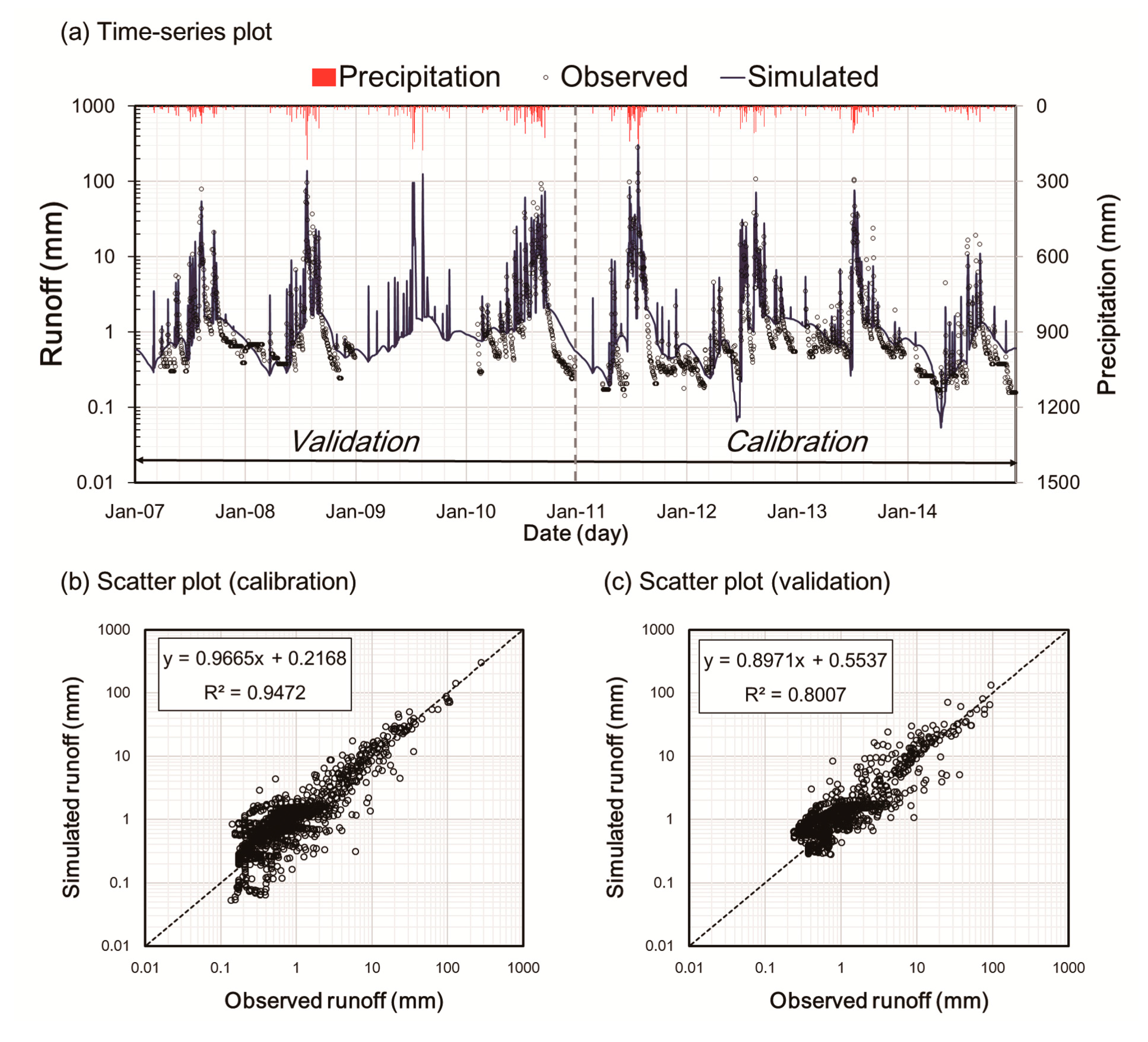
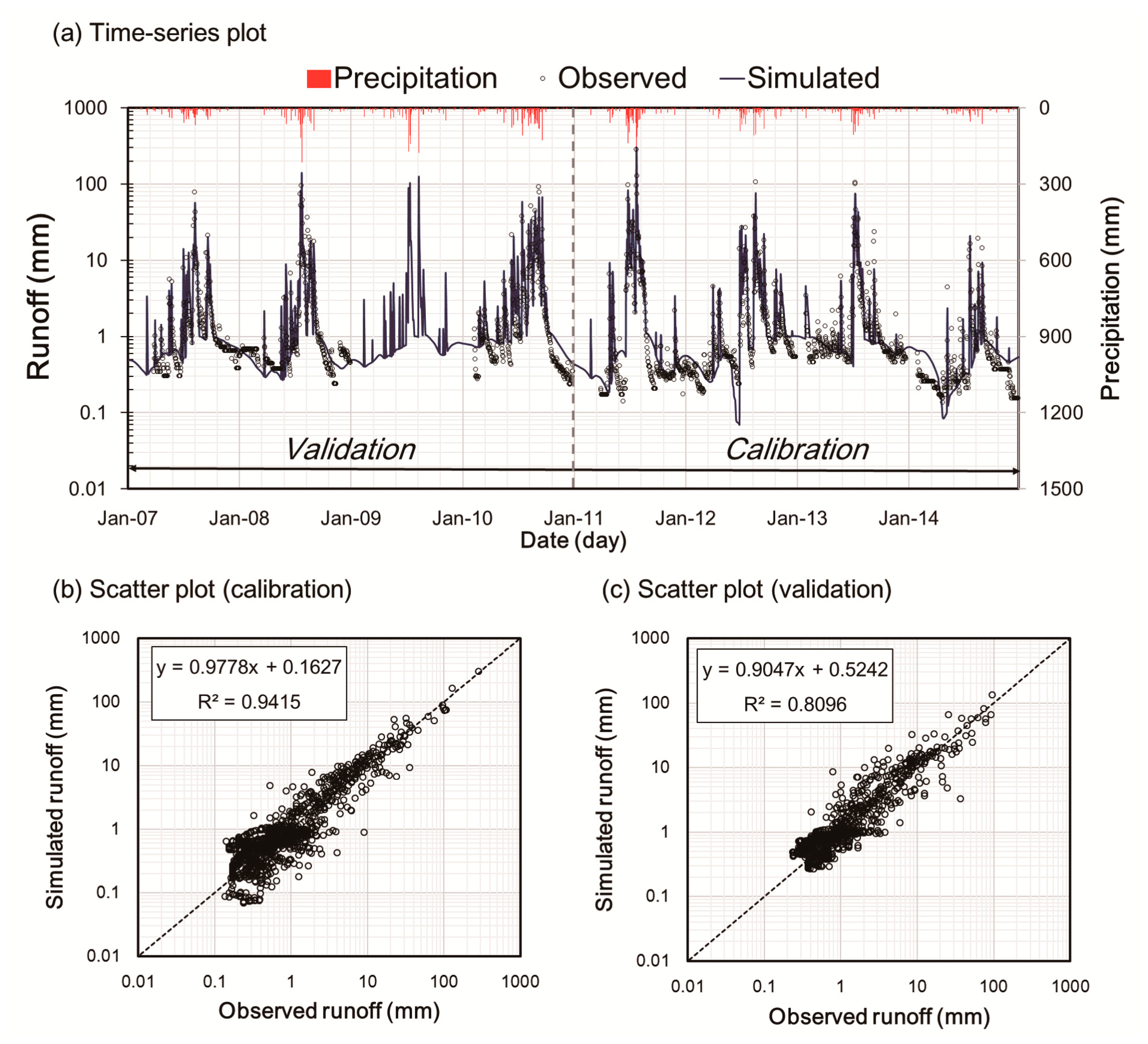
5.2.2. Optimization Results
6. Conclusions
Acknowledgments
Author Contributions
Conflicts of Interest
References
- Singh, V.P.; Woolhiser, D.A. Mathematical modeling of watershed hydrology. J. Hydrol. Eng. 2002, 7, 270–292. [Google Scholar] [CrossRef]
- Kang, M.S.; Srivastava, P.; Song, J.H.; Park, J.; Her, Y.; Kim, S.M.; Song, I. Development of a Component-Based Modeling Framework for Agricultural Water-Resource Management. Water 2016, 8, 351. [Google Scholar] [CrossRef]
- Sugawara, M. Automatic calibration of the tank model. Hydrol. Sci. J. 1979, 24, 375–388. [Google Scholar] [CrossRef]
- Lindström, G.; Johansson, B.; Persson, M.; Gardelin, M.; Bergström, S. Development and test of the distributed HBV-96 hydrological model. J. Hydrol. 1997, 201, 272–288. [Google Scholar] [CrossRef]
- Moore, R.J. The probability-distributed principle and runoff production at point and basin scales. Hydrol. Sci. J. 1985, 30, 273–297. [Google Scholar] [CrossRef]
- Zhao, R.J. The Xinanjiang model applied in China. J. Hydrol. 1992, 135, 371–381. [Google Scholar] [CrossRef]
- Abbott, M.B.; Bathurst, J.C.; Cunge, J.A.; O’Connell, P.E.; Rasmussen, J. An introduction to the European Hydrological System—Systeme Hydrologique Europeen,“SHE”, 1: History and philosophy of a physically-based, distributed modelling system. J. Hydrol. 1986, 87, 45–59. [Google Scholar] [CrossRef]
- Young, R.A.; Onstad, C.A.; Bosch, D.D.; Anderson, W.P. AGNPS: A nonpoint-source pollution model for evaluating agricultural watersheds. J. Soil Water Conserv. 1989, 44, 168–173. [Google Scholar]
- Beasley, D.B.; Huggins, L.F.; Monke, A. ANSWERS: A model for watershed planning. Trans. ASAE 1980, 23, 938–0944. [Google Scholar] [CrossRef]
- Beven, K. Changing ideas in hydrology—The case of physically-based models. J. Hydrol. 1989, 105, 157–172. [Google Scholar] [CrossRef]
- Orth, R.; Staudinger, M.; Seneviratne, S.I.; Seibert, J.; Zappa, M. Does model performance improve with complexity? A case study with three hydrological models. J. Hydrol. 2015, 523, 147–159. [Google Scholar] [CrossRef] [Green Version]
- Gurtz, J.; Zappa, M.; Jasper, K.; Lang, H.; Verbunt, M.; Badoux, A.; Vitvar, T. A comparative study in modelling runoff and its components in two mountainous catchments. Hydrol. Process. 2003, 17, 297–311. [Google Scholar] [CrossRef]
- Kobierska, F.; Jonas, T.; Zappa, M.; Bavay, M.; Magnusson, J.; Bernasconi, S.M. Future runoff from a partly glacierized watershed in Central Switzerland: A two-model approach. Adv. Water Resour. 2013, 55, 204–214. [Google Scholar] [CrossRef]
- Khakbaz, B.; Imam, B.; Hsu, K.; Sorooshian, S. From lumped to distributed via semi-distributed: Calibration strategies for semi-distributed hydrologic models. J. Hydrol. 2012, 418, 61–77. [Google Scholar] [CrossRef]
- Rumbaugh, J.; Blaha, M.; Premerlani, W.; Eddy, F.; Lorensen, W. Object-Oriented Modeling and Design; Prentice-Hall: Upper Saddle River, NJ, USA, 1991. [Google Scholar]
- Argent, R.M.; Voinov, A.; Maxwell, T.; Cuddy, S.M.; Rahman, J.M.; Seaton, S.; Vertessy, R.A.; Braddock, R.D. Comparing modelling frameworks—A workshop approach. Environ. Model. Softw. 2006, 21, 895–910. [Google Scholar] [CrossRef]
- Clements, P.C. From subroutines to subsystems: Component-based software development. Am. Program. 1995, 8, 1–8. [Google Scholar]
- Zeigler, B.P. Object-Oriented Simulation with Hierarchical Modular Models; Academic Press: San Diego, CA, USA, 1990. [Google Scholar]
- Maxwell, T. A parsi-model approach to modular simulation. Environ. Model. Softw. 1999, 14, 511–517. [Google Scholar] [CrossRef]
- Muhanna, W.A. SYMMS: A model management system that supports model reuse, sharing, and integration. Eur. J. Oper. Res. 1994, 72, 214–243. [Google Scholar] [CrossRef]
- Guariso, G.; Hitz, M.; Werthner, H. An integrated simulation and optimization modelling environment for decision support. Decis. Support Syst. 1996, 16, 103–117. [Google Scholar] [CrossRef]
- Bennett, D.A. A framework for the integration of geographical information systems and model base management. Int. J. Geogr. Inf. Sci. 1997, 11, 337–357. [Google Scholar] [CrossRef]
- Reed, M.; Cuddy, S.M.; Rizzoli, A.E. A framework for modelling multiple resource management issues—An open modelling approach. Environ. Model. Softw. 1999, 14, 503–509. [Google Scholar] [CrossRef]
- Mantecón, J.A.; Gómez, M.; Rodellar, J. A Simulink-based scheme for simulation of irrigation canal control systems. Simulation 2002, 78, 485–493. [Google Scholar] [CrossRef]
- Kinnucan, P.; Mosterman, P.J. A graphical variant approach to object-oriented modeling of dynamic systems. In Proceedings of the 2007 Summer Computer Simulation Conference, Society for Computer Simulation International, San Diego, CA, USA, 16–19 July 2007. [Google Scholar]
- Bowen, J.D.; Perry, D.N.; Bell, C.D. Hydrologic and Water Quality Model Development Using Simulink. J. Mar. Sci. Eng. 2014, 2, 616–632. [Google Scholar] [CrossRef]
- Romanowicz, R. A Matlab implementation of TOPMODEL. Hydrol. Process. 1997, 11, 1115–1129. [Google Scholar] [CrossRef]
- Lanini, S.; Courtois, N.; Giraud, F.; Petit, V.; Rinaudo, J.D. Socio-hydrosystem modelling for integrated water-resources management-the Hėrault catchment case study, southern France. Environ. Model. Softw. 2004, 19, 1011–1019. [Google Scholar] [CrossRef]
- Chappell, N.A.; Tych, W.; Bonell, M. Development of the forSIM model to quantify positive and negative hydrological impacts of tropical reforestation. For. Ecol. Manag. 2007, 251, 52–64. [Google Scholar] [CrossRef]
- Wolfs, V.; Meert, P.; Willems, P. Modular conceptual modelling approach and software for river hydraulic simulations. Environ. Model. Softw. 2015, 71, 60–77. [Google Scholar] [CrossRef]
- MATLAB Documentation. Available online: mathworks.com/help (accessed on 9 March 2017).
- Paik, K.; Kim, J.H.; Kim, H.S.; Lee, D.R. A conceptual rainfall-runoff model considering seasonal variation. Hydrol. Process. 2005, 19, 3837–3850. [Google Scholar] [CrossRef]
- Jang, T.; Kim, H.; Kim, S.; Seong, C.; Park, S. Assessing irrigation water capacity of land use change in a data-scarce watershed of Korea. J. Irrig. Drain. Eng. 2011, 138, 445–454. [Google Scholar] [CrossRef]
- Fumikazu, N.; Toshisuke, M.; Yoshio, H.; Hiroshi, T.; Kimihito, N. Evaluation of water resources by snow storage using water balance and tank model method in the Tedori River basin of Japan. Paddy Water Environ. 2013, 11, 113–121. [Google Scholar] [CrossRef]
- Song, J.H.; Kang, M.S.; Song, I.; Jun, S.M. Water balance in irrigation reservoirs considering flood control and irrigation efficiency variation. J. Irrig. Drain Eng. 2016, 142, 04016003. [Google Scholar] [CrossRef]
- Wang, S.; Huang, G.H.; Baetz, B.W.; Ancell, B.C. Towards robust quantification and reduction of uncertainty in hydrologic predictions: Integration of particle Markov chain Monte Carlo and factorial polynomial chaos expansion. J. Hydrol. 2017, 548, 484–497. [Google Scholar] [CrossRef]
- Jung, D.; Choi, Y.H.; Kim, J.H. Multiobjective Automatic Parameter Calibration of a Hydrological Model. Water 2017, 9, 187. [Google Scholar] [CrossRef]
- Kim, H.Y.; Park, S.W. Simulating daily inflow and release rates for irrigation reservoirs. J. Korean Soc. Agric. Eng. 1988, 30, 50–62. (In Korean) [Google Scholar]
- Huh, Y.M. A Streamflow Network Model for Daily Water Supply and Demands on Small Watershed. Ph.D. Thesis, Seoul National University, Seoul, Korea, 1992. [Google Scholar]
- Schrader, F.; Durner, W.; Fank, J.; Gebler, S.; Pütz, T.; Hannes, M.; Wollschläger, U. Estimating precipitation and actual evapotranspiration from precision lysimeter measurements. Procedia Environ. Sci. 2013, 19, 543–552. [Google Scholar] [CrossRef]
- Rahimi, S.; Gholami, S.M.A.; Raeini-Sarjaz, M.; Valipour, M. Estimation of actual evapotranspiration by using MODIS images (a case study: Tajan catchment). Arch. Agron. Soil Sci. 2015, 61, 695–709. [Google Scholar] [CrossRef]
- Valipour, M. Comparative evaluation of radiation-based methods for estimation of potential evapotranspiration. J. Hydrol. Eng. 2014, 20, 04014068. [Google Scholar] [CrossRef]
- Thornthwaite, C.W. An approach toward a rational classification of climate. Geogr. Rev. 1948, 38, 55–94. [Google Scholar] [CrossRef]
- Blaney, H.F.; Criddle, W.D. Determining Consumptive Use and Irrigation Water Requirements; No. 1275; US Department of Agriculture: Washington, DC, USA, 1962.
- Jensen, M.E.; Haise, H.R. Estimating evapotranspiration from solar radiation. J. Irrig. Drain. Div. 1963, 89, 15–41. [Google Scholar]
- Hargreaves, G.H.; Samani, Z.A. Estimating potential evapotranspiration. J. Irrig. Drain. Div. 1982, 108, 225–230. [Google Scholar]
- Penman, H.L. Natural evaporation from open water, bare soil and grass. In Proceedings of the Royal Society of London, A: Mathematical, Physical, and Engineering Sciences, London, UK, 22 April 1948. [Google Scholar]
- Allen, R.G.; Pereira, L.S.; Raes, D.; Smith, M. Crop Evapotranspiration-Guidelines for Computing Crop Water Requirements-FAO Irrigation and Drainage Paper 56; Food and Agriculture Organization: Rome, Italy, 1998. [Google Scholar]
- Priestley, C.H.B.; Taylor, R.J. On the assessment of surface heat flux and evaporation using large-scale parameters. Mon. Weather Rev. 1972, 100, 81–92. [Google Scholar] [CrossRef]
- Yu, P.S.; Yang, T.C.; Chou, C.C. Effects of climate change on evapotranspiration from paddy fields in southern Taiwan. Clim. Chang. 2002, 54, 165–179. [Google Scholar] [CrossRef]
- Sung, S.H. Determination of Evapotranspiration Ratio to Estimate Actual Evapotranspiration in Small Forested-Watersheds. Master’s Thesis, Seoul National University, Seoul, Korea, 1997. (In Korean). [Google Scholar]
- Yoo, S.H.; Choi, J.Y.; Jang, M.W. Estimation of paddy rice crop coefficients for FAO Penman-Monteith and Modified Penman method. J. Korean Soc. Agric. Eng. 2006, 48, 13–23. (In Korean) [Google Scholar]
- Nonsaro. Available online: nongsaro.go.kr (accessed on 24 August 2017).
- Park, S.W. A Tank model shell program for simulating daily streamflow from small watershed. J. Korea Water Resour. Assoc. 1993, 26, 47–61. (In Korean) [Google Scholar]
- Oudin, L.; Hervieu, F.; Michel, C.; Perrin, C.; Andréassian, V.; Anctil, F.; Loumagne, C. Which potential evapotranspiration input for a lumped rainfall–runoff model? Part 2—Towards a simple and efficient potential evapotranspiration model for rainfall–runoff modelling. J. Hydrol. 2005, 303, 290–306. [Google Scholar] [CrossRef]
- Clark, M.P.; Kavetski, D.; Fenicia, F. Pursuing the method of multiple working hypotheses for hydrological modeling. Water Resour. Res. 2011, 47, 9. [Google Scholar] [CrossRef]
- Van Esse, W.; Perrin, C.; Booij, M.; Augustijn, D.; Fenicia, F.; Kavetski, D.; Lobligeois, F. The influence of conceptual model structure on model performance: A comparative study for 237 French catchments. Hydrol. Earth Syst. Sci. 2013, 17, 4227–4239. [Google Scholar] [CrossRef] [Green Version]
- Gan, T.Y.; Dlamini, E.M.; Biftu, G.F. Effects of model complexity and structure, data quality, and objective functions on hydrologic modeling. J. Hydrol. 1997, 192, 81–103. [Google Scholar] [CrossRef]
- Moriasi, D.N.; Arnold, J.G.; Van Liew, M.W.; Bingner, R.L.; Harmel, R.D.; Veith, T.L. Model evaluation guidelines for systematic quantification of accuracy in watershed simulations. Trans. ASABE 2007, 50, 885–900. [Google Scholar] [CrossRef]
- Chapman, S.J. MATLAB Programming for Engineers; Nelson Education: Scarborough, ON, Canada, 2015. [Google Scholar]
- Engel, B.; Storm, D.; White, M.; Arnold, J.; Arabi, M. A hydrologic/water quality model application protocol. J. Am. Water Resour. Assoc. 2007, 43, 1223–1236. [Google Scholar] [CrossRef]
- Moriasi, D.N.; Gitau, M.W.; Pai, N.; Daggupati, P. Hydrologic and water quality models: Performance measures and evaluation criteria. Trans. ASABE 2015, 58, 1763–1785. [Google Scholar] [CrossRef]
- Madsen, H. Automatic calibration of a conceptual rainfall–runoff model using multiple objectives. J. Hydrol. 2000, 235, 276–288. [Google Scholar] [CrossRef]
- Nash, J.; Sutcliffe, J.V. River flow forecasting through conceptual models part I-A discussion of principles. J. Hydrol. 1970, 10, 282–290. [Google Scholar] [CrossRef]
- Oudin, L.; Andreassian, V.; Mathevet, T.; Perrin, C.; Michel, C. Dynamic averaging of rainfall-runoff model simulations from complementary model parameterizations. Water Resour. Res. 2006, 42, 7. [Google Scholar] [CrossRef]
- Perrin, C.; Michel, C.; Andréassian, V. Improvement of a parsimonious model for streamflow simulation. J. Hydrol. 2003, 279, 275–289. [Google Scholar] [CrossRef]
- Pushpalatha, R.; Perrin, C.; Le Moine, N.; Andreassian, V. A review of efficiency criteria suitable for evaluating low-flow simulations. J. Hydrol. 2012, 420, 171–182. [Google Scholar] [CrossRef]


| Parameter | Alpha | |||||||||||
|---|---|---|---|---|---|---|---|---|---|---|---|---|
| Min. | 0 | 0.08 | 0.08 | 5 | 20 | 0.1 | 0.03 | 0 | 0.01 | 0.003 | 0 | 0 |
| Max. | 0.5 | 0.5 | 0.5 | 60 | 110 | 0.5 | 0.5 | 100 | 0.35 | 0.03 | 0 | 0.11 |
| Crop Coeff. | January | February | March | April | May | June | July | August | September | October | November | December |
|---|---|---|---|---|---|---|---|---|---|---|---|---|
| Forest | 0.47 | 0.46 | 0.55 | 0.59 | 0.74 | 0.72 | 0.87 | 1.01 | 0.98 | 0.87 | 0.64 | 0.45 |
| Paddy | 0.20 | 0.20 | 0.20 | 0.65 | 0.70 | 0.99 | 1.30 | 1.17 | 0.83 | 0.20 | 0.20 | 0.20 |
| Upland | 0.36 | 0.36 | 0.37 | 0.37 | 0.58 | 0.78 | 0.82 | 0.82 | 0.76 | 0.57 | 0.37 | 0.36 |
| Others | 0.20 | 0.20 | 0.20 | 0.20 | 0.20 | 0.20 | 0.20 | 0.20 | 0.20 | 0.20 | 0.20 | 0.20 |
| Year | 2007 | 2008 | 2009 | 2010 | 2011 | 2012 | 2013 | 2014 |
|---|---|---|---|---|---|---|---|---|
| Rainfall (mm) | 1260 | 1458 | 1541 | 1977 | 2211 | 1481 | 1448 | 767 |
| Case | Period | (%) | |||
|---|---|---|---|---|---|
| 1 | Calibration | 0.95 | 0.95 | −0.15 | −4.4 |
| Validation | 0.80 | 0.79 | 0.34 | −7.5 | |
| 2 | Calibration | 0.94 | 0.94 | 0.07 | −3.6 |
| Validation | 0.81 | 0.80 | 0.57 | −7.3 |
© 2017 by the authors. Licensee MDPI, Basel, Switzerland. This article is an open access article distributed under the terms and conditions of the Creative Commons Attribution (CC BY) license (http://creativecommons.org/licenses/by/4.0/).
Share and Cite
Song, J.-H.; Her, Y.; Park, J.; Lee, K.-D.; Kang, M.-S. Simulink Implementation of a Hydrologic Model: A Tank Model Case Study. Water 2017, 9, 639. https://doi.org/10.3390/w9090639
Song J-H, Her Y, Park J, Lee K-D, Kang M-S. Simulink Implementation of a Hydrologic Model: A Tank Model Case Study. Water. 2017; 9(9):639. https://doi.org/10.3390/w9090639
Chicago/Turabian StyleSong, Jung-Hun, Younggu Her, Jihoon Park, Kyung-Do Lee, and Moon-Seong Kang. 2017. "Simulink Implementation of a Hydrologic Model: A Tank Model Case Study" Water 9, no. 9: 639. https://doi.org/10.3390/w9090639
APA StyleSong, J.-H., Her, Y., Park, J., Lee, K.-D., & Kang, M.-S. (2017). Simulink Implementation of a Hydrologic Model: A Tank Model Case Study. Water, 9(9), 639. https://doi.org/10.3390/w9090639