Article

Hysteresis Curve Fitting Optimization of Magnetic Controlled Shape Memory Alloy Actuator

College of Machinery and Automation, Wuhan University of Science and Technology, Wuhan 430081, China
*
Author to whom correspondence should be addressed.
Actuators 2016, 5(4), 25; https://doi.org/10.3390/act5040025
Submission received: 2 September 2016 / Revised: 12 October 2016 / Accepted: 2 November 2016 / Published: 8 November 2016
(This article belongs to the Special Issue MEMS-based Actuators)

Abstract

:
As a new actuating material, magnetic controlled shape memory alloys (MSMAs) have excellent characteristics such as a large output strain, fast response, and high energy density. These excellent characteristics are very attractive for precision positioning systems. However, the availability of MSMAs in practical precision positioning is poor, caused by weak repeatability under a certain stimulus. This problem results from the error of a large magnetic hysteresis in an external magnetic field. A suitable hysteresis modelling method can reduce the error and improve the accuracy of the MSMA actuator. After analyzing the original hysteresis modelling methods, three kinds of hysteresis modelling methods are proposed: least squares method, back propagation (BP) artificial neural network, and BP artificial neural network based on genetic algorithms. Comparing the accuracy and convergence rate of three kinds of hysteresis modelling methods, the results show that the convergence rate of least squares method is the fastest, and the convergence accuracy of BP artificial neural networks based on genetic algorithms is the highest.

Graphical Abstract

1. Introduction

During the end of last century, Ullakko et al. [1] found and proposed a magnetic controlled shape memory alloy (MSMA). Then, Murray et al. [2,3] conducted research into the mechanism and characteristics of MSMA. When a sample of MSMA is placed in a suitable external magnetic field, it can produce a deformation as high as 10%. Moreover, compared with traditional shape memory alloys, MSMA has characteristics of larger strain and better energy efficiency. These excellent characteristics are very attractive for precision positioning systems [4]. Since then, some scholars and organizations have designed many kinds of MSMA actuators. However, there are still relatively few applications for MSMA actuators in precision positioning. The deficiency in practical precision positioning is caused by the weak repeatability under a certain stimulus. This is the result of the error caused by a large magnetic hysteresis [5,6] in an external magnetic field. To reveal the hysteresis characteristic of MSMA [7], related experiments with NiMnGa (which is the typical MSMA material) are carried out.
According to the research and analysis of Spanish scholars, suitable hysteresis modelling methods can reduce errors and improve the accuracy of MSMA actuators [8]. Thus, it is very important to reference and establish hysteresis modelling methods.
At present, several kinds of commonly hysteresis models exist:
(1)
Preisach model: Preisach model [9,10,11] can fit a complex hysteresis curve. However, for some materials, the fitting error is large.
(2)
Jiles–Atherton model: The advantage of the Jiles–Atherton model [12,13] is its excellent convergence, while the disadvantage is that it is difficult to achieve fast modelling due to numerous undetermined parameters.
(3)
Maxwell model: Maxwell model [14,15] can improve the convergence rate by reducing the number of subsystems, but the accuracy of the model is reduced accordingly.
In addition, the proportional-integral-derivative (PID) model and other models recently became research hotspots [16,17,18]. To date, none of the modelling methods developed is perfect. By analyzing the original hysteresis modelling methods, three kinds of hysteresis modelling methods are proposed for fitting the hysteresis curve: least squares method [19], back propagation (BP) artificial neural network and BP artificial neural network based on genetic algorithm. Among these methods, there are special improvements. First, BP artificial neural network that adopts the Levenberg–Marquard algorithm is a novel method and has some advantages: (a) because the Levenberg–Marquard algorithm is a type of least squares method, it can it can be directly used for fitting the hysteresis curve; (b) mean square error of the Levenberg–Marquard algorithm [20] can be used to test the rate of convergence and error size; therefore, it can be used to test the reliability and accuracy of the BP artificial neural network. Moreover, the basic principle of BP artificial neural network based on a genetic algorithm [21,22] is as follows: through the selection, crossover and mutation operation of genetic algorithms, optimize the weights and thresholds of the neural network, and then return the optimal weights and the optimal thresholds to the BP artificial neural network. By comparing the precision of fitting the hysteresis curve, the best hysteresis modelling method will be selected.

2. Performance Experiment of MSMA Actuator

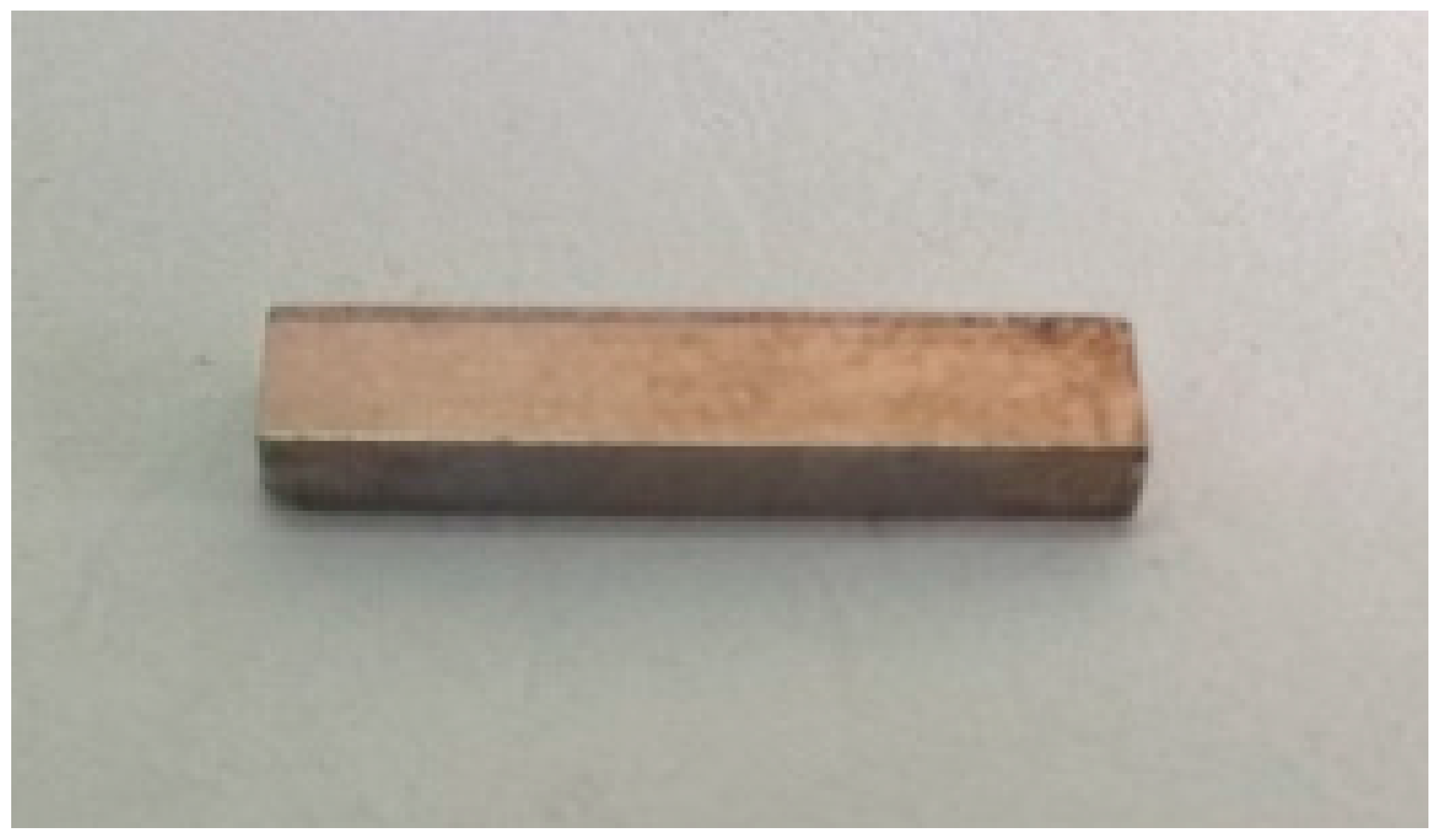
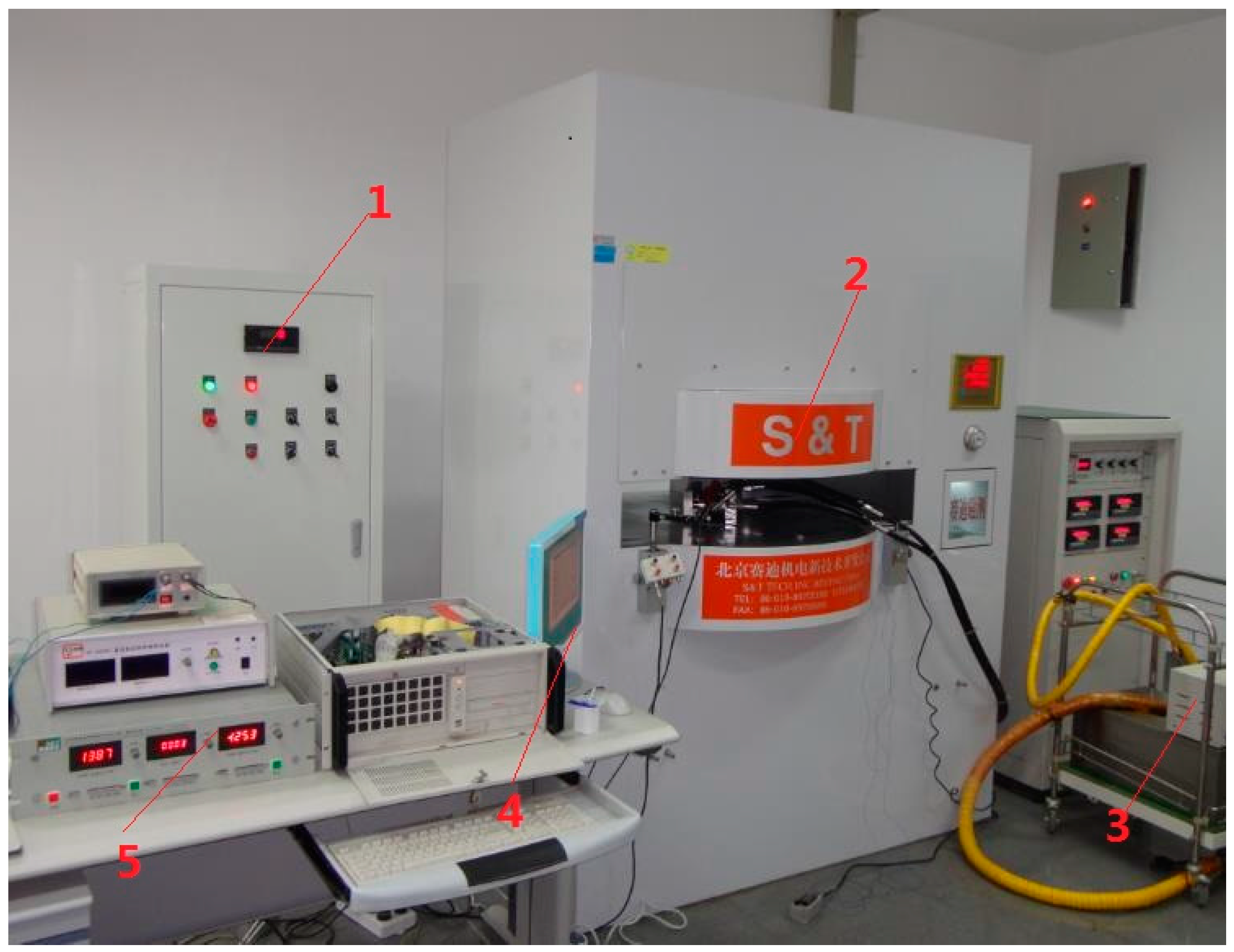
2.1. Sample and Device of the Experiment

The sample of MSMA in the experiment is an NiMnGa alloy purchased from the Goodfellow company (Huntingdon, UK). The overall dimensions of the sample are 2 × 3 × 15 mm 3 , and its appearance is shown in Figure 1. Moreover, the atomic percentages of the Ni element, Mn element, and Ga element are 50%, 28%, and 22%, respectively.
This experiment adopts a magnetic force coupling thermal loading measuring system (shown in Figure 2) to study multifield coupling properties of force and magnetic field of the MSMA under variable temperature magnetics. During the experiment, the load is provided by a hydraulic system and is measured by a force sensor. Moreover, the load ranges from 0 to 2.5 MPa. The external control magnetic field is provided by an electric current: the magnetic field range is 0–1.5 T, and the current is proportional to the magnetic field. The operating temperature is regulated by a circulating oil bath temperature loading system, and the working temperature range is 16–35 °C. When the magnetic field is perpendicular or parallel to the preload stress, axial and transverse deformation of the MSMA sample will be produced. These will be measured with a resistance strain gauge. The basic characteristics of the resistance strain gauge are as follows:
(1)
The strain gauge is a series of BX (BX strain gauge refers to phenolic foil type strain gauge) whose properties include the following: the entire structure is sealed, stable performance, good flexibility, and applicability to the general accuracy of the sensor. The strain limit is 1.5%, and usage temperature range is −30 °C–+80 °C.
(2)
The strain gauge sampling frequency is 4 Hz.
Experimental steps are as follows:
(1)
Turn off the power, place the sample in the cup, and fix the cup on the hydraulic loading device intermediate.
(2)
The hydraulic drive loading device is directly placed in the working range. At the same time, the magnetic field is set from 0 to 1.5 T.
(3)
Turn on the power, and set up the pre load of the sample.
(4)
Turn on the power supply for the temperature loading system, set the temperature parameters, and check whether the outer circulation system makes good contact. When everything is acceptable, turn on the heating power supply and the oil pump power supply, and regulate the flow rate of silicone oil circulation to prevent the silicone oil spilling.
(5)
Start the test. The corresponding deformation of MSMA is measured.
(6)
After unloading, view and save the experimental data.

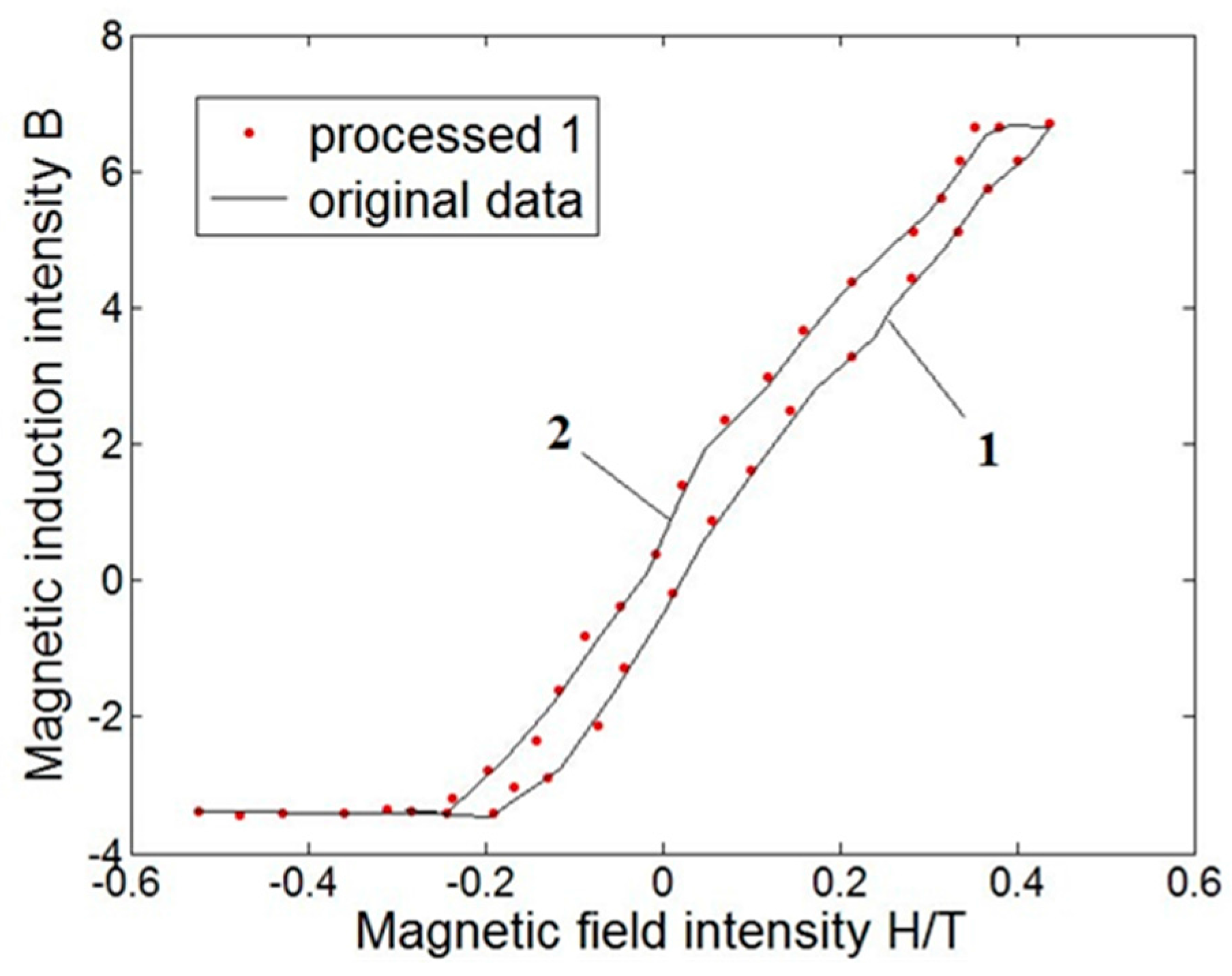
2.2. Experimental Results

In order to achieve good experimental results, the experimental conditions must meet the following requirements. First, magnetic field intensity H is parallel to the external load. The operating temperature is 16 °C, and the size of external load is 3.9 kg. In the experimental conditions, the key original experimental data of magnetic field intensity H and magnetic induction intensity B are shown in Table 1.

3. Fitting and Results

3.1. Least Squares Method

As we know, MATLAB software (MATLAB 2013, MathWorks Company, Natick, MA, USA) is the most common software numerical calculation and graphics processing. In this chapter, we apply the least squares method with MATLAB software to fit the original experimental data.
Compared with some other least squares methods, we adopt the quadratic polynomial method for the following reasons. First, the quadratic polynomial method is one of the most common least squares methods. Second, the calculation time for the quadratic polynomial method is the shortest of the least squares methods. In this paper, we assume a fitting equation as follows:
y = a 4 x 4 + a 3 x 3 + a 2 x 2 + a 1 x + a 0 .
The programming procedure to fit the original experimental data is as follows:
clear
a = load(”data.txt”);
x = a(:, 1);
y = a(:, 2);
P = polyfit(x, y, 4)
Application results of the programming procedure are shown as follows:
P = [−8.2964, −33.4283, 8.7761, 17.8643, 0.0325]
Therefore,
a 4 = 8.2964 , a 3 = 33.4283 , a 2 = 8.7761 , a 1 = 17.8643 , a 0 = 0.0325 .
Using Equation (1), the mathematical equation of the fitting curve is as follows:
y = 8.2964 x 4 33.4283 x 3 + 8.7761 x 2 + 17.8643 x + 0.0325
Through a simulation analysis using MATLAB software, the fitting curve and the original experimental data curve are shown in Figure 3.
Through the original experimental data curve in Figure 3, magnetic induction intensity B is maintained at approximately −3.4 T when magnetic field intensity H ranges from −0.25 T to −0.54 T. Shown as curve 1 in Figure 3, magnetic induction intensity B gradually increases from −3.4 T to 6.8 T when magnetic field intensity H ranges from −0.25 T to 0.4 T. However, shown as curve 2 in Figure 3, magnetic induction intensity B gradually decreases from 6.8 T to −3.4 T when magnetic field intensity H ranges from 0.4 T to −2.5 T. Obviously, curve 1 and curve 2 do not coincide. Therefore, as shown in Figure 3, the relation curve between magnetic field intensity H and magnetic induction intensity B is the hysteresis curve of the MSMA.
With regard to Equation (2), because the number of undetermined parameters during the hysteresis curve fitting is lower, the fitting speed of the least squares method is faster. A wealth of information can be found in the statistics figures. For example, with regard to Figure 3 and Figure 4, the fitting curve using the least squares method can show the trend of the hysteresis curve as 0.33% of the largest fitting error rate.
More importantly, the largest fitting error rate of 0.33% is quite accurate and can improve the accuracy of the MSMA actuator. In order to further improve the fitting accuracy of the fitting curve, this paper adopts a BP artificial neural network to carry out the fitting.

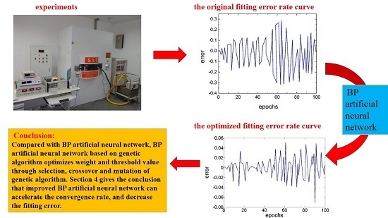
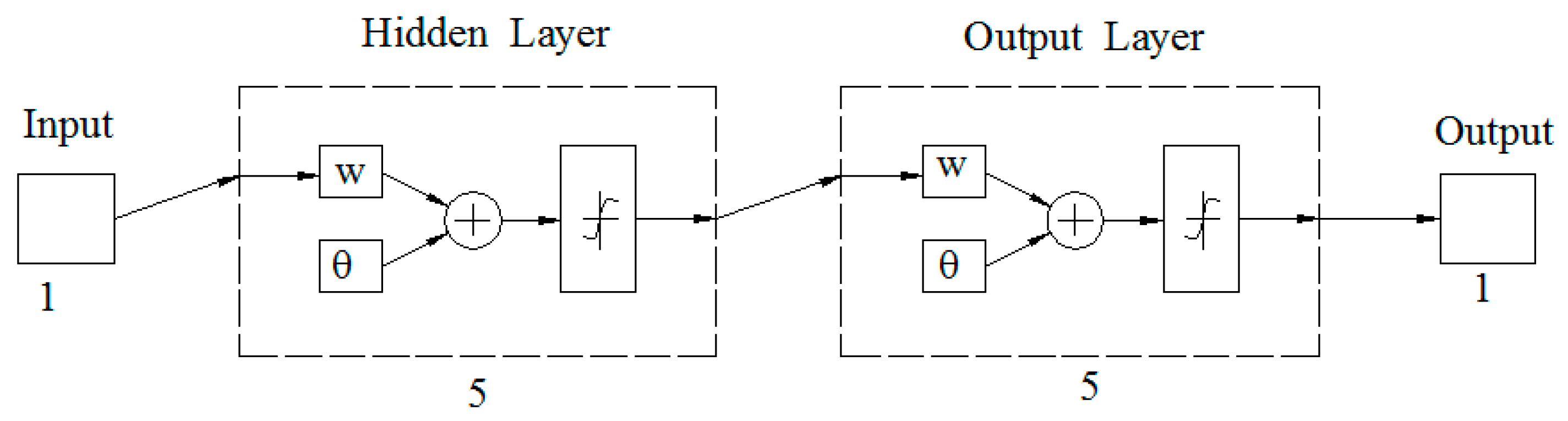
3.2. BP Artificial Neural Network

This paper adopts a three-layer BP artificial neural network. The network is divided into an input layer, hidden layer, and output layer. The input and output layers are, respectively, magnetic field intensity H and magnetic induction intensity B. The number of input layer nodes and output layer nodes are both 1. Like the least squares method, we apply a BP artificial neural network with MATLAB software to fit the original experimental data. We apply equation calculations combined with programming algorithms to establish a magnetic hysteresis model that is faster and more accurate.
Through various analyses, the number of hidden layer nodes is determined as
m = a + b + c .
In Equation (3), a and b are, respectively, the number of input layer nodes and output layer nodes. In addition, c ranges from 1 to 10. When c is 3, the number of hidden layer nodes is 5. Therefore, the structure of the artificial neural network is 1-5-1, as shown in Figure 5.
The activation function of neurons g(x) in the hidden layer is a bipolar compressed function:
g ( x ) = 1 2 + 1 1 + e λ x .
Correspondingly, the activation function of neurons h(x) in the output layer is a symmetric saturated linear satlins function:
h ( x ) = { 1 , , x < 1 x ,   1 x 1   1 , x 1 .
In this paper, the original BP artificial neural network that adopts the Levenberg–Marquard algorithm has some advantages: (a) because the Levenberg–Marquard algorithm is a type of least squares method, it can be directly used for fitting the hysteresis curve; and the (b) mean square error of the Levenberg–Marquard algorithm can be used to test the rate of convergence and error size; therefore, it can be used to test the reliability and accuracy of the BP artificial neural network.
The equation for mean square error E m s e in the Levenberg–Marquard algorithm is
E m s e = 1 n i = 1 n ( o r i g i e x p i ) 2 .
In Equation (6), o r i g i is original experimental data, and e x p i is expected data. If mean square error E m s e is important, equally so is weight adjustment Δ w :
Δ w = [ J T ( W ) J ( W ) + μ 1 I ] 1 J T ( W ) e ( w ) ,
where I is the unit matrix, μ 1 is the user-defined learning rate, e ( w ) is the error vector, and J ( W ) is the jacobian reciprocal matrix of the error to weights, as shown in Equation (8):
J ( W ) = | e 1 ( x ) w 1 e 1 ( x ) w 2 e 2 ( x ) w 1 e 2 ( x ) w 2 e 1 ( x ) w n e 2 ( x ) w n e n ( x ) w 1 e n ( x ) w 2 e n ( x ) w n | .
Moreover, the equation of threshold adjustment Δ θ is shown in Equation (9):
Δ θ = μ 2 f ( θ T x ) x ,
where μ 2 is the user-defined learning rate, x is the input vector, and f ( θ T x ) is the output of the neurons.
Through an analysis of the activation function, weight adjustment, and threshold adjustment, this paper uses MATLAB software to realize a hysteresis curve fitting based on a BP artificial neural network.
The fitting curve and the original experimental data curve are shown in Figure 6.
As shown in Figure 7, the fitting error rate between the fitting curve and the original experimental data curve has large fluctuations. It was found that the largest fitting error rate for the original BP artificial neural network (0.07%) is much smaller than the largest fitting error rate through the least squares method (0.33%).
To further analyse the fitting effect using an original BP artificial neural network, the mean square error is introduced. As shown in Figure 8, the mean square error sharply decreases during 0–10 iterations. After 10 iterations, the mean square error slows until it stops changing. Finally, the mean square error reaches its minimum of 9.9413   ×   10 5 at the 100th iteration. Therefore, compared with the least squares method, the BP artificial neural network based on a genetic algorithm can decrease the fitting error and improve the accuracy of the MSMA actuator. In addition, its convergence rate is relatively slow.

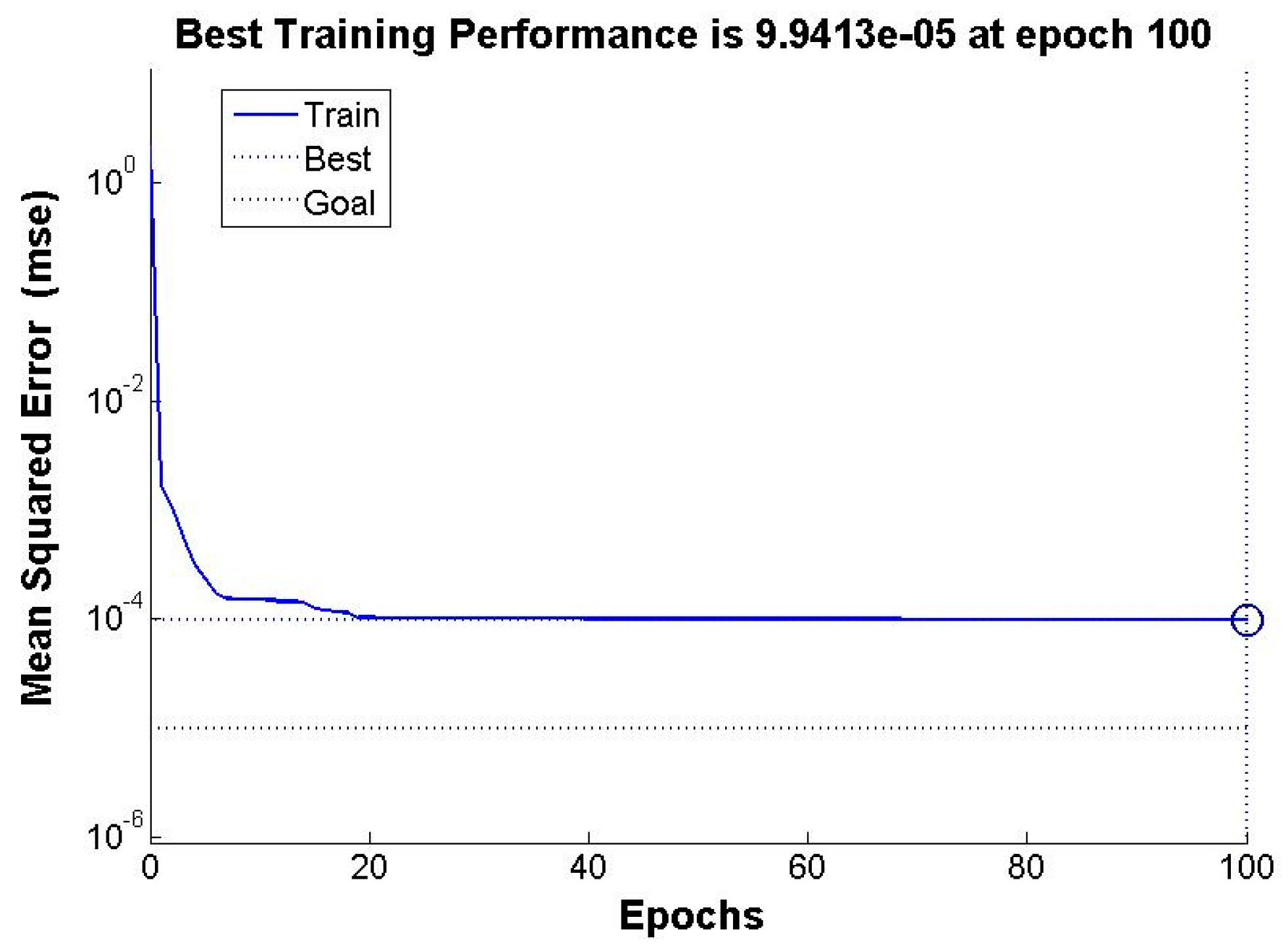
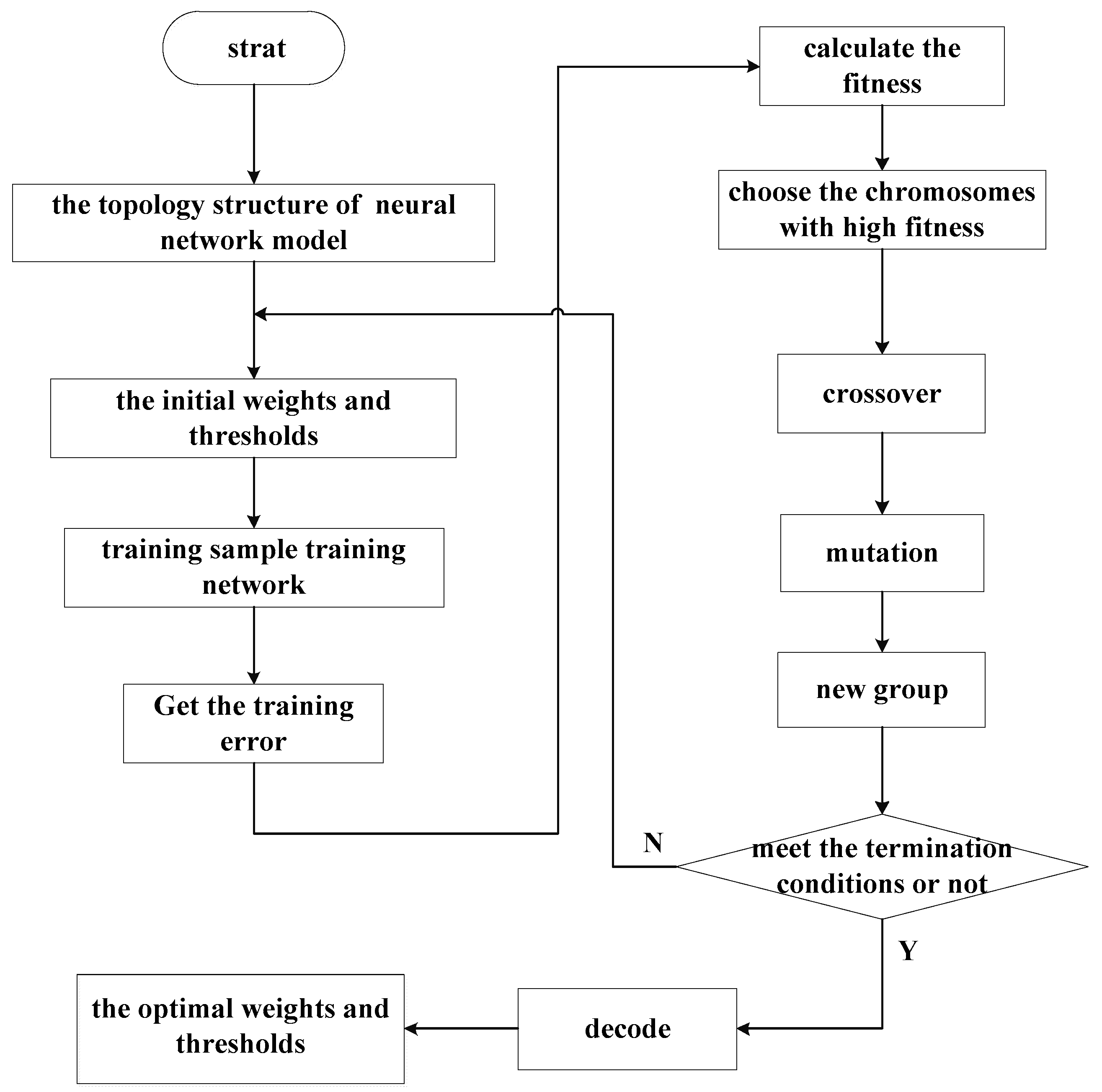
3.3. BP Artificial Neural Network Based on Genetic Algorithm
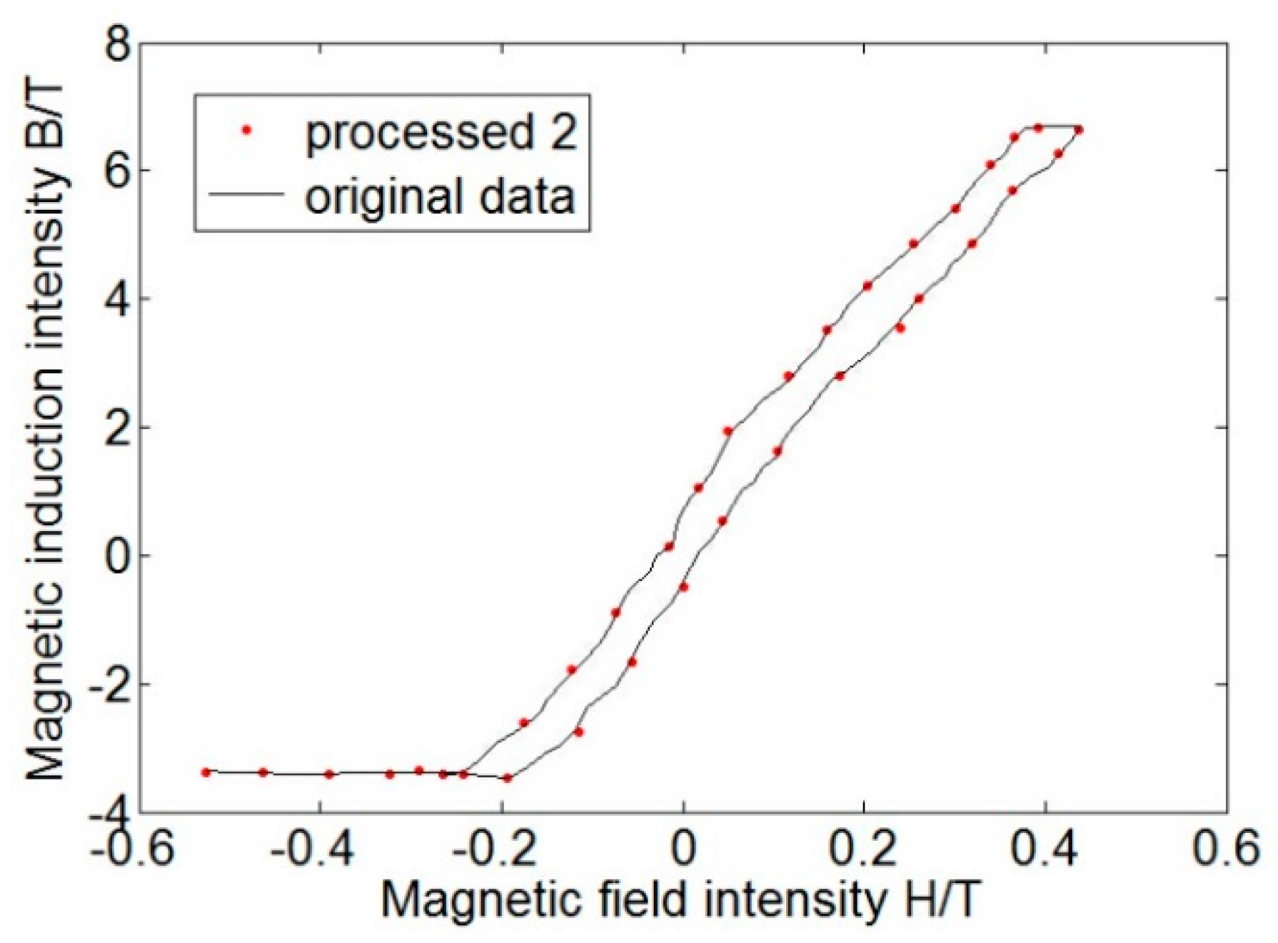
Based on an analysis of Figure 7 and Figure 8, the convergence at the 100th iteration is slow, and 0.07% of the largest fitting-error rate is not small.
In order to accelerate the convergence rate of the original BP artificial neural network, this paper uses a genetic algorithm to improve BP artificial neural network. As shown in Figure 9, the weight and threshold values of the BP artificial neural network are optimized through selection, crossover, and mutation of the genetic algorithm.
In this paper, the initial parameters of genetic algorithm are as follows: the population size is 20, crossover probability is 0.1, and mutation probability is 0.0001.
Through selection, crossover and mutation of genetic algorithm, the optimized weight and threshold value are as follows:
W 1 = [ 2.0774 ,   2.7653 ,   1.6402 ,   3.3241 ,   3.1488 ] T ,
W 2 = [ 0.0032 ,   1.8282 ,   1.8009 ,   0.6494 ,   0.9973 ] ,
θ 1 = [ 2.7870 ,   0.1735 ,   1.3575 ,   0.3503 ,   0.6810 ] T ,
θ 2 = [ 0.6449 ] .
The following require special attention: W 1 in Equation (10) is the weight between the input layer and the hidden layer, W 2 in Equation (11) is the weight between the hidden layer and the output layer, θ 1 in Equation (11) is the threshold value between the input layer and the hidden layer, and θ 2 in Equation (12) is the threshold value between the hidden layer and the output layer.
As shown in Figure 10, it is found that 0.03% of the largest fitting error rate through an improved BP artificial neural network is much smaller than 0.33% of the largest fitting error rate through an original BP artificial neural network.
To further show the advantages of the BP artificial neural network based on a genetic algorithm, as shown in Figure 11, the mean square error of the BP artificial neural network based on a genetic algorithm reaches its minimum of 4.9804   ×   10 5 at the 16th iteration. Compared with the mean-square-error curve of the original BP artificial neural network in Figure 8, a BP artificial neural network based on a genetic algorithm not only accelerates the convergence rate but also decreases the fitting error.
Therefore, it can improve the accuracy of the MSMA actuator and then enhance the utilization rate of the MSMA actuator in precision positioning.

4. Validation

To validate the reliability and accuracy of the BP neural network based on a genetic algorithm, this paper makes use of additional original experimental data in experimental conditions. The experimental conditions are as follows: magnetic field intensity H is parallel to the external load; operating temperature is 16 °C; the size of the external load is 4.9 kg; and the range of the magnetic field intensity H is 0–1 T.
To test the fitting effect, through a simulation analysis using MATLAB software, the fitting curve and the original experimental data curve are shown in Figure 12. As preliminarily seen in Figure 12, the fitting accuracy of the BP neural network based on a genetic algorithm is excellent.
As shown in Figure 13, the largest fitting error rate of BP artificial neural network is 0.06%, and the largest fitting error rate of the BP artificial neural network based on a genetic algorithm is 0.025%. Thus, a BP artificial neural network based on a genetic algorithm can significantly reduce the fitting error.
To further show the advantage of the BP artificial neural network based on a genetic algorithm, as shown in Figure 14, the mean square error of the BP artificial neural network based on a genetic algorithm reaches its minimum of 5.0384 × 10⁻⁵ at the 19th iteration. There is no doubt that a BP artificial neural network based on a genetic algorithm can accelerate the convergence rate and decrease the fitting error.

5. Conclusions

Through the above experiments and simulation analysis, the conclusions are as follows:
(1)
The fitting accuracy rate is quite high and can improve the accuracy of MSMA actuators. Because there are fewer undetermined parameters during the hysteresis curve fitting, the fitting speed of least squares method is fast.
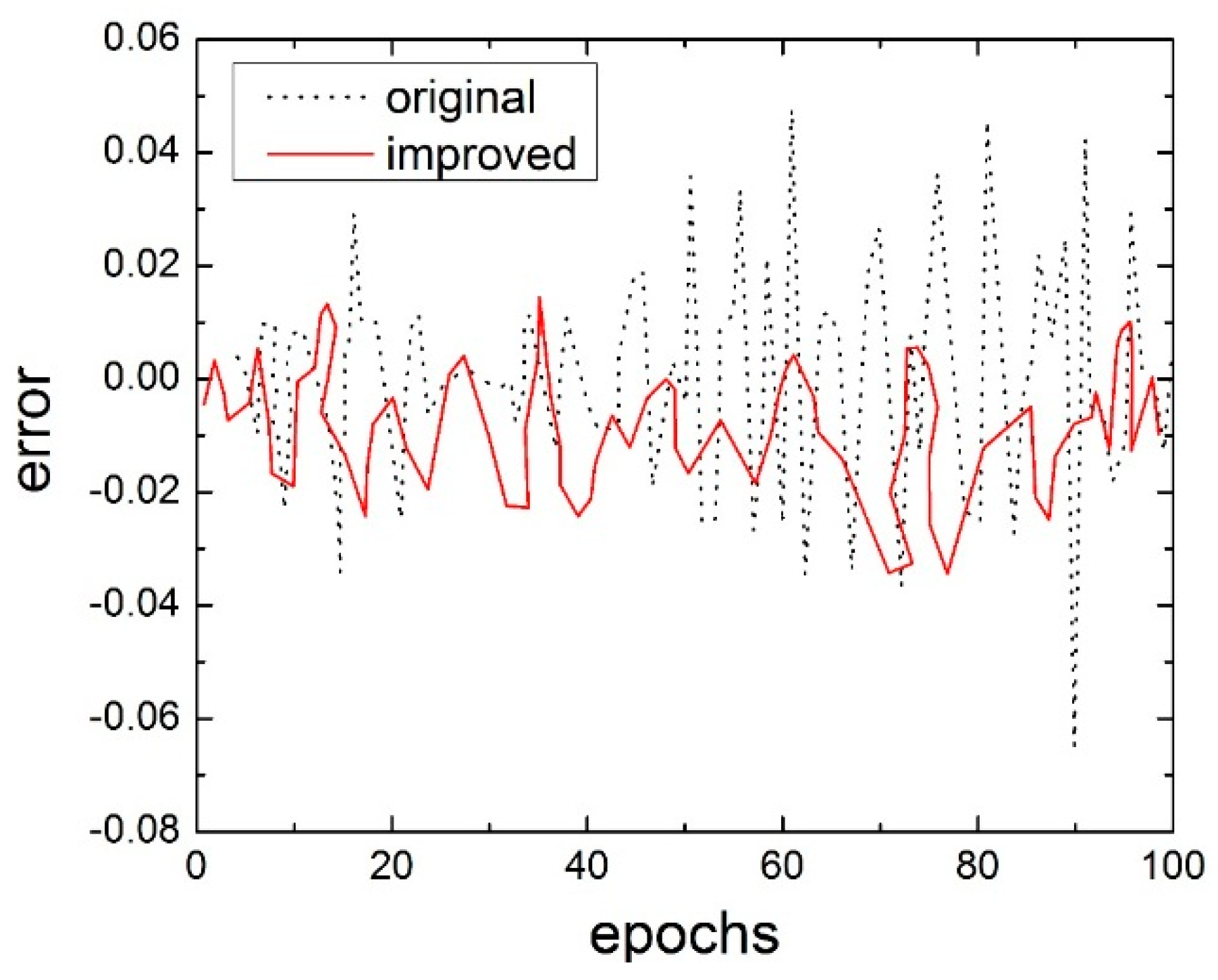
(2)
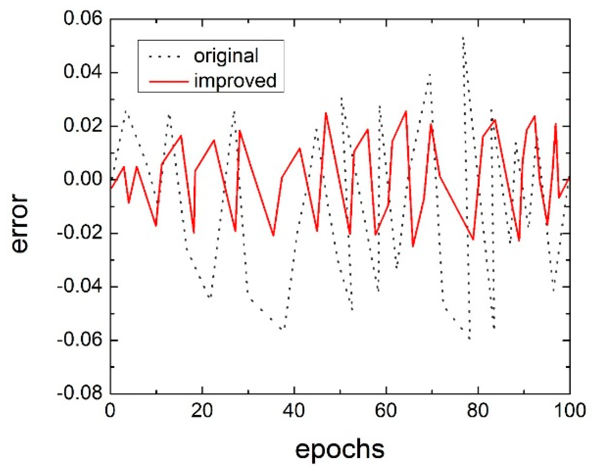
Compared with BP artificial neural networks, BP artificial neural networks based on genetic algorithms can accelerate the convergence rate and decrease the fitting error. Therefore, they can improve the accuracy of MSMA actuators and enhance the utilization rate of MSMA actuators in precision positioning.

Acknowledgments

This study was funded by the China National Natural Science Funding Project (Grant No: 51274155) and Hubei Province Natural Science Funding Project (Grant No: 2015CFA114).

Author Contributions

F.T. and S.H. conceived and designed the experiments; Y.Z. and Y.W. performed the experiments; J.L. analyzed the data; Z.S. contributed analysis tools; S.H. wrote the paper.

Conflicts of Interest

The authors declare no conflict of interest.

References

  1. Ullakko, K.; Huang, J.K.; Kantner, C.; O’Handley, R.C.; Kokorin, V.V. Large magnetic-field-induced strains in Ni2MnGa single crystals. Appl. Phys. Lett. 1996, 69, 1966–1968. [Google Scholar] [CrossRef]
  2. Murray, S.J.; Marioni, M.; Allen, S.M.; O’Handley, R.C.; Lograsso, T.A. 6% magnetic-field-induced strain by twin-boundary motion in ferromagnetic Ni–Mn–Ga. Appl. Phys. Lett. 2000, 77, 886–888. [Google Scholar] [CrossRef]
  3. Murray, S.J.; Farinelli, M.; Kantner, C.; Huang, J.K.; Allen, S.M.; O’Handley, R.C. Field-induced strain under load in Ni-Mn-Ga magnetic shape memory materials. J. Appl. Phys. 1998, 83, 7297–7299. [Google Scholar] [CrossRef]
  4. Feuchtwanger, J.; Asua, E.; García-Arribas, A.; Etxebarria, V.; Barandiaran, J.M. Ferromagnetic shape memory alloys for positioning with nanometric resolution. Appl. Phys. Lett. 2009, 95, 054102. [Google Scholar] [CrossRef]
  5. Murray, S.J.; Marioni, M.; Tello, P.G.; O’Handley, R.C. Giant magnetic-field-induced strain in Ni–Mn–Ga crystals: Experimental results and modelling. J. Magn. Magn. Mater. 2001, 226, 945–947. [Google Scholar] [CrossRef]
  6. Conti, S.; Lenz, M.; Rumpf, M. Hysteresis in magnetic shape memory composites: Modelling and simulation. J. Mech. Phys. Solids 2016, 89, 272–286. [Google Scholar] [CrossRef]
  7. Krenke, T.; Aksoy, S.; Duman, E.; Acet, M.; Moya, X.; Mañosa, L.; Planes, A. Hysteresis effects in the magnetic-field-induced reverse martensitic transition in magnetic shape-memory alloys. J. Appl. Phys. 2010, 108, 043914. [Google Scholar] [CrossRef]
  8. Sadeghzadeh, A.; Asua, E.; Feuchtwanger, J.; Etxebarria, V.; García-Arribas, A. Ferromagnetic shape memory alloy actuator enabled for nanometric position control using hysteresis compensation. Sens. Actuators A Phys. 2012, 182, 122–129. [Google Scholar] [CrossRef]
  9. Tao, G. Adaptive control of systems with nonsmooth input and output nonlinearities. IEEE Trans. Autom. Control 1996, 41, 1348–1352. [Google Scholar]
  10. Ossart, F.; Davidson, R.; Charap, S.H. A 3D moving vector Preisach hysteresis model. IEEE Trans. Magn. 1995, 31, 1785–1788. [Google Scholar] [CrossRef]
  11. Sutor, A.; Rupitsch, S.J.; Lerch, R. A Preisach-based hysteresis model for magnetic and ferroelectric hysteresis. Appl. Phys. A 2010, 100, 425–430. [Google Scholar] [CrossRef]
  12. Takahashi, N.; Miyabara, S.H.; Fujiwara, K. Problems in practical finite element analysis using Preisach hysteresis model. IEEE Trans. Magn. 1999, 35, 1243–1246. [Google Scholar] [CrossRef] [Green Version]
  13. Annakkage, U.D.; McLaren, P.G.; Dirks, E.; Jayasinghe, R.P.; Parker, A.D. A current transformer model based on the Jiles–Atherton theory of ferromagnetic hysteresis. IEEE Trans. Power Deliv. 2000, 15, 57–61. [Google Scholar] [CrossRef]
  14. Toman, M.; Stumberger, G.; Dolinar, D. Parameter identification of the Jiles–Atherton hysteresis model using differential evolution. IEEE Trans. Magn. 2008, 44, 1098–1101. [Google Scholar] [CrossRef]
  15. Rao, I.J.; Rajagopal, K.R. On a new interpretation of the classical Maxwell model. Mech. Res. Commun. 2007, 34, 509–514. [Google Scholar] [CrossRef]
  16. Zhou, M.; Zhang, Q. Hysteresis Model of Magnetically Controlled Shape Memory Alloy Based on a PID Neural Network. IEEE Trans. Magn. 2015, 51, 1–4. [Google Scholar]
  17. Zhou, M.; He, S.; Zhang, Q.; Ji, K.; Hu, B. Hybrid control of magnetically controlled shape memory alloy actuator based on Krasnosel’skii–Pokrovskii model. J. Intell. Fuzzy Syst. 2015, 29, 63–73. [Google Scholar] [CrossRef]
  18. Zhou, M.; He, S.; Hu, B.; Zhang, Q. Modified KP model for hysteresis of magnetic shape memory alloy actuator. IETE Tech. Rev. 2015, 32, 29–36. [Google Scholar] [CrossRef]
  19. Liu, Y.; Liu, H.; Wu, H.; Zou, D. Modelling and compensation of hysteresis in piezoelectric actuators based on Maxwell approach. Electron. Lett. 2015, 52, 188–190. [Google Scholar] [CrossRef]
  20. Shi, Y.; Liang, C.H. The finite-volume time-domain algorithm using least squares method in solving Maxwell’s equations. J. Comput. Phys. 2007, 226, 1444–1457. [Google Scholar] [CrossRef]
  21. Wilamowski, B.M.; Iplikci, S.; Kaynak, O.; Efe, M.Ö. An algorithm for fast convergence in training neural networks. In Proceedings of the International Joint Conference on Neural Networks, Washington, DC, USA, 15–19 July 2001; Volume 3, pp. 1778–1782.
  22. Fu, Z.; Mo, J.; Chen, L.; Chen, W. Using genetic algorithm-back propagation neural network prediction and finite-element model simulation to optimize the process of multiple-step incremental air-bending forming of sheet metal. Mater. Des. 2010, 31, 267–277. [Google Scholar] [CrossRef]
Figure 1. Sample of magnetic controlled shape memory alloy (MSMA) for the experiment.
Actuators 05 00025 g001
Figure 2. Experimental setup: (1) power; (2) loading device; (3) power supply for temperature loading system; (4) computer with data acquisition card, which collects input magnetic field intensity H and output magnetic induction intensity B; and (5) control device for magnetic field.
Actuators 05 00025 g002
Figure 3. Fitting curve and original experimental data curve. ”Processed 1” represents the fitting curve through least squares method. ”Original data” represents the original experimental data.
Actuators 05 00025 g003
Figure 4. The fitting error rate curve of the least squares method.
Actuators 05 00025 g004
Figure 5. Structure of the back propagation (BP) artificial neural network.
Actuators 05 00025 g005
Figure 6. Fitting curve and original experimental data curve. “Processed 2” represents the fitting curve through the original BP artificial neural network. “Original data” represents the original experimental data curve.
Actuators 05 00025 g006
Figure 7. Fitting-error-rate curve for the original BP artificial neural network.
Actuators 05 00025 g007
Figure 8. Mean square error curve.
Actuators 05 00025 g008
Figure 9. Flowchart of the improved original BP artificial neural network.
Actuators 05 00025 g009
Figure 10. Fitting-error-rate curve. “Original” and “improved” represent the fitting-error-rate curve of the BP artificial neural network and BP artificial neural network based on genetic algorithms, respectively.
Actuators 05 00025 g010
Figure 11. Mean square error curve of the BP artificial neural network based on genetic algorithms.
Actuators 05 00025 g011
Figure 12. Fitting curve and the original experimental data curve. “Processed 4” represents the fitting curve through the BP neural network based on a genetic algorithm. “Original data” represents the original experimental data.
Actuators 05 00025 g012
Figure 13. Fitting error rate curve of the BP artificial neural network and the BP artificial neural network based on genetic algorithms.
Actuators 05 00025 g013
Figure 14. The mean square error curve of the BP artificial neural network based on a genetic algorithm.
Actuators 05 00025 g014
Table 1. Key original experimental data.
Serial NumberH (T)B (T)Serial NumberH (T)B (T)Serial NumberH (T)B (T)
1−0.5258−3.4152110.03010.2790210.07071.9553
2−0.4640−3.3831120.05030.8144220.04461.2415
3−0.31118−3.4097130.09661.4583230.00700.6694
4−0.2506−3.4061140.12842.065624−0.01330.0627
5−0.1235−2.7931150.20663.281225−0.0857−1.2237
6−0.0887−2.0787160.32524.926626−0.1088−1.6881
7−0.0569−1.6138170.44396.714527−0.1754−2.7962
8−0.0395−1.1853180.37416.702828−0.2188−3.3261
9−0.0134−0.7208190.21264.4432
100.0096−0.2920200.16923.6708

