Article

Mapping the Soil Salinity Distribution and Analyzing Its Spatial and Temporal Changes in Bachu County, Xinjiang, Based on Google Earth Engine and Machine Learning

1
College of Resources and Environment, Xinjiang Agricultural University, Urumqi 830052, China
2
Xinjiang Laboratory of Soil and Plant Ecological Processes, Urumqi 830052, China
*
Author to whom correspondence should be addressed.
Agriculture 2024, 14(4), 630; https://doi.org/10.3390/agriculture14040630
Submission received: 11 March 2024 / Revised: 9 April 2024 / Accepted: 10 April 2024 / Published: 19 April 2024
(This article belongs to the Section Digital Agriculture)

Abstract

:
Soil salinization has a significant impact on agricultural production and ecology. There is an urgent demand to establish an effective method that monitors the spatial and temporal distribution of soil salinity. In this study, a multi-indicator soil salinity monitoring model was proposed for monitoring soil salinity in Bachu County, Kashgar Region, Xinjiang, from 2002 to 2022. The model was established by combining multiple predictors (spectral, salinity, and composite indices and topographic factors) and the accuracy of the four models (Random Forest [RF], Partial Least Squares [PLS], Classification Regression Tree [CART], and Support Vector Machine [SVM]) was compared. The results reveal the high accuracy of the optimized prediction model, and the order of the accuracy is observed as RF > PLS > CART > SVM. The most accurate model, RF, exhibited an R2 of 0.723, a root mean square error (RMSE) of 2.604 g·kg−1, and a mean absolute error (MAE) of 1.95 g·kg−1 at a 0–20 cm depth. At a 20–40 cm depth, RF had an R2 value of 0.64, an RMSE of 3.62 g·kg−1, and an MAE of 2.728 g·kg−1. Spatial changes in soil salinity were observed throughout the study period, particularly increased salinization from 2002 to 2012 in the agricultural and mountainous areas within the central and western regions of the country. However, salinization declined from 2012 to 2022, with a decreasing trend in salinity observed in the top 0–20 cm of soil, followed by an increasing trend in salinity at a 20–40 cm depth. The proposed method can effectively extract large-scale soil salinity and provide a practical basis for simplifying the remote sensing monitoring and management of soil salinity. This study also provides constructive suggestions for the protection of agricultural areas and farmlands.

1. Introduction

Soil salinization is currently a serious environmental problem faced globally [1]. It profoundly impacts agricultural production, ecological equilibrium, and sustainable development [2,3,4]. Soil salinization affects over 20% of the world’s irrigated farmland [5], with more than half concentrated in four countries: China, India, Pakistan, and the United States of America [6]. In China, inland areas face more severe salinization hazards than coastal regions, particularly in locales with scarce water resources. Therefore, understanding soil salinity levels is crucial for determining optimal irrigation timing, implementing effective management practices, ensuring soil quality, fostering robust plant growth, and conserving water resources [7]. Given this context, conducting a comprehensive examination of the spatial and temporal dynamics of salinization has emerged as a pressing imperative to safeguard land resources, preserve ecological equilibrium, and ensure agricultural productivity.
Conventional approaches for soil salinity measurements typically involve collecting field soil samples for laboratory analysis to determine solute concentrations. However, such methods are time-consuming and costly [3,8,9,10]. In recent years, the application of remote sensing techniques to assess soil salinity has increased [11,12] due to their short measurement time, extensive monitoring range, and capacity to acquire multi-temporal data. In particular, remote sensing technology offers efficient and cost-effective tools for rapid soil salinity monitoring. Monitoring techniques can be classified into two categories, namely, direct assessments of bare soil and indirect assessments through vegetation affected by soil salinity [13]. Recently, scholars have determined a correlation between vegetation growth information and soil salinity concentration via vegetation indices [14]. Furthermore, an increasing number of studies have adopted the salinity index and its composite index for soil salinity monitoring [15,16]. Utilizing environmental variables such as elevation, slope, and aspect has great potential for accurately identifying salinized soils [17]. Previous research has demonstrated a correlation between these indicators and soil salinity indices [18]. Numerous scholars have predicted soil salinity by establishing a relationship between various indices (e.g., spectral indices) and measured soil salinity, selecting the optimal inversion factors, and constructing inversion models through diverse satellite remote sensing data [19,20].
The majority of previous related research relies on empirical models. However, Google Earth Engine (GEE) offers corrected global Landsat series data combined with machine learning algorithm interfaces. These resources enable the application of large-scale machine learning [21,22,23] and deep learning [24,25] approaches that utilize extensive cloud data and computing power. Such models enhance the capability to monitor soil salinization. Moreover, scholars have used vegetation indices to construct models in GEE to study soil salinization [26]. Currently, the integration of GEE and machine learning is being employed for cropland mapping [27,28], surface temperature estimation [29], and classification monitoring [30]. However, multivariate studies of soil salinization inversions continue to use traditional empirical models and processing tools such as ENVI (Esri). While the monitoring accuracy of such models is satisfactory, there remains room for streamlining the analysis processes. The traditional process for monitoring salinity through remote sensing is generally divided into three stages. The first stage involves preprocessing remote sensing data. The second stage includes screening sensitive factors using correlation analysis and other methods. In the third stage, optimal factors are determined, and regression or machine learning algorithms are employed for modeling. Traditionally, this process requires the use of multiple software tools. However, the GEE cloud computing platform provides an all-in-one solution, facilitating machine learning algorithm-based modeling and empirical modeling. Previous research has primarily concentrated on surface soil model development, with limited attention focused on estimating soil salinity at various depths using remote sensing data. Furthermore, spatial analysis of soil salinity has been the primary focus of past studies, while temporal monitoring remains overlooked.
Hence, this study introduces a comprehensive and streamlined approach to soil salinity monitoring. A multi-parameter remote sensing prediction model was developed for long-term soil salinity monitoring at varying depths in Bachu, Xinjiang. This model utilized multi-year Landsat 5, Landsat 8, and Landsat 9 imagery from 2002 to 2022, along with measured soil salinity data at the depths of 0–20 cm and 20–40 cm. This study maximizes the utilization of the GEE remote sensing platform, integrating ground-based soil salinity measurements with machine learning to perform robust remote sensing monitoring of soil salinization. The proposed approach adopts environmental factors and vegetation, spectral, and composite indices as variables. The research objectives of this study are to (1) optimize the predictor selection from multiple types of variables; (2) evaluate the accuracy of the empirical and machine learning models across different soil depths; and (3) generate spatial and temporal distribution maps of soil salinity in topsoil and deep-soil layers in Bachu County and analyze their spatial and temporal variations.

2. Materials and Methods

2.1. Overview of the Study Area

The study area (38.427°–40.187° N and 77.227°–79.567° E) is located in the southwestern part of the Xinjiang Uygur Autonomous Region, at the southern foothills of the Tianshan Mountains and the northwestern margin of the Tarim Basin. Situated in the Asian–European continent’s hinterland, it shares borders with Aksu Prefecture to the east; Shache County, Mageti County, and the Hotan region to the south; Gashi County, Yephu County, and Kizilsu and Kirghiz Autonomous Prefectures to the west; and extends to the Keping Mountain in the north, part of the Tien Shan Mountain system. The terrain in the study area slopes from the southwest to the northeast and contains four key geomorphological categories, namely, deserts, mountains, flood plains, and alluvial plains. With an average temperature of 11.9 °C, an annual precipitation average of 60 mm, an annual evapotranspiration average of 3218.2 mm, and 2500–3000 annual sunshine hours, the area exhibits a dry climate, high evapotranspiration rates, and significant diurnal temperature fluctuations, classifying it as a temperate continental dry climate. Bachu County, situated in Xinjiang, is a sizable agricultural area characterized by arid conditions, leading to significant surface salt accumulation and water scarcity. Hence, efficient soil salinity monitoring in this region is crucial for promoting regional water conservation and facilitating the development of arid regions. Bachu County has large areas of saline-tolerant plants, such as poplar forests, which can grow in saline soils and harsh climatic conditions, and therefore grow thickly in such saline areas [31]. Soil salinization is one of the main drivers of desertification. Bachu County is located on the northwestern edge of the Taklamakan Desert and is thus faced with the problem of desertification, exacerbating the risk of soil salinization. Conducting salinization testing can help identify areas with potential desertification risk in a timely manner, thus helping to protect the ecological environment. Moreover, combining soil spatial planning with salinization testing can optimize land use and improve the efficiency of land resource utilization [32].

2.2. Technological Approach

This study utilizes the GEE cloud computing platform along with the machine learning algorithms and remote sensing data provided by GEE. Thirty-one indices were extracted and correlated with soil salinity at the measured sampling points depicted in Figure 1. Six optimal factors were selected and incorporated into four models. The optimal model was then employed to analyze the spatial and temporal changes in soil salinity across different depths in Bachu County. The data processing and analysis flow is depicted in Figure 2.

2.3. Data Sources and Processing

2.3.1. Ground-Truth Data

The ground-truth data of soil salinity used in this study were obtained from field sampling in the spring of 2002, 2010, and 2022. In the field collection of composite soil samples, the five-point sampling method was adopted, in which five surface soil samples were randomly selected in each sample plot, crushed and mixed together, then one sample was formed by removing impurities such as roots, mulch, rocks, etc., and each sample point was collected at two depths, namely, 0~20 cm and 20~40 cm, respectively. A total of 124 sample points were measured in the field, including soil salt content, soil pH, and other data, of which 64 sample points were centrally distributed in the southwest and west of Bachu County next to farmland and rivers, 36 sample points were distributed in the northeast and south of Bachu County in the bare land, desert, and rocky and bare soil areas, and the remaining 24 sample points were distributed in the sparsely vegetated central and eastern areas, such as grasslands and shrublands. The land cover types of the sample sites covered all land types in Batchelor County. The sampling sites for the 2022 field measurement validation data were evenly distributed within the study area (Figure 1). The measured soil salinity values of the field sampling sites were classified according to the classification criteria of soil salinity, which resulted in 26 non-saline, 33 mildly saline, 31 moderately saline, 21 heavily saline, and 13 saline soil sample sites, and the criteria for classifying the soil salinity grades are detailed in Table 1 [33].

2.3.2. Remote Sensing Data

Landsat 7 and Landsat 9, the latest generation of Landsat data, were selected as the main data sources for the study; see Table 2 for details. Atmospheric correction was performed on these datasets using the LEDAPS and LaSRC algorithms. Masking of clouds, shadows, water, and snow was then performed based on the saturation of each pixel by the CFMASK (C version of the Function of Mask) method. The satellite products were obtained through the GEE platform. The composite index was also extracted after calculation in the GEE platform. All datasets were obtained from the same period as the sampling points (2002, 2012, and spring 2022) [34].

2.3.3. Spectral Indices

We extracted the raw spectral information of six bands from the Landsat 5, Landsat 8, and Landsat 9 imagery, namely, the blue (Blue, 0.45–0.51 μm), green (Green, 0.53–0.59 μm), red (Red, 0.64–0.67 μm), near-infrared (NIR, 0.85–0.88 μm), short-wave infrared 1 (SWIR1, 1.57–1.65 μm), and short-wave infrared 2 (SWIR2, 2.11–2.29 μm) bands.
In arid regions characterized by sparse vegetation and extensive surface fragmentation, the selection of a suitable vegetation index significantly impacts the accuracy of vegetation remote sensing estimations. Two key factors must be accounted for when choosing a vegetation index: its capability to minimize soil background interference and its effectiveness in detecting low-cover vegetation. The most commonly used vegetation index is the normalized difference vegetation index (NDVI) [35], which responds to the health status of vegetation and to invert soil salinity. In this study, we combined the NDVI with the difference vegetation index (DVI), which is strong in detecting low-coverage vegetation, and the modified soil-adjusted vegetation index (MSAVI), which regulates the influence of the soil background well, to construct the model. We also employed the enhanced normalized difference vegetation index (ENDVI), the enhanced red vegetation index (ERVI), and the canopy redness index (CRSI), which have been reported to have better performances in soil salinity monitoring. Table 3 presents the calculation formulas of these indices.

2.3.4. Salinity Indices

Salinity indices are highly correlated with soil salinization and are usually determined from remotely sensed data. In this study, we use salinity indices to quantify the degree and distribution of soil salinization in Bachu County. These indices can reflect the effect of soil salinization on the surface of Albedo, thus helping us to understand the spatial distribution characteristics of soil salinization [41]. Table 4 reports the 11 salinity indices (SIs), namely, SI1–SI9, NDSI, and SI-T, used in this study.

2.3.5. Composite Indices

Previous research has demonstrated the applicability of inversion factors derived from Albedo-MSAVI and SI1-NDVI eigenspaces for investigating soil salinity in arid regions [51]. In this study, these factors are denoted as AM and SDI, respectively. This study employed two composite indices derived from the feature space. The indices were computed using the SI1, NDVI, and Albedo metrics, as described in Table 4. To maintain data consistency in the subsequent analyses, normalization of SI1, NDVI, MSAVI, and Albedo was performed using the following equation:
n X = X X min X m a x X min ,
where nX denotes the normalized value of X; X refers to the values of SI1, NDVI, MSAVI, and Albedo, respectively; X m a x and X min denote the maximum and minimum values of SI1, NDVI, MSAVI, and Albedo, respectively. Composite index formula, as shown in Table 5.

2.3.6. Topographic Factors

Topography is important in soil formation, serving as a reflection of the interaction between water flow and soil characteristics. Quantitative topographic factors have been utilized in predicting soil properties [55]. In particular, elevation influences human activity frequency. In sparsely inhabited regions at higher elevations, vegetation growth typically thrives, boasting higher overall coverage, thereby significantly impacting soil salinity dynamics. Similarly, slope gradient and orientation shape plant growth, indirectly affecting soil salinity levels. Hence, utilizing the topography of Bachu County, we extracted topographic data, specifically the SRTM digital elevation model (DEM), from the GEE platform. Three key factors—elevation, slope, and aspect—were derived.

2.3.7. Climatic Factors

Precipitation and evaporation exert significant influences on the rate and extent of soil salinization [56]. Therefore, we focused on evaporation and precipitation as key environmental variables. This study utilized the MOD16A2.061 dataset retrieved from MODIS (Moderate Resolution Imaging Spectroradiometer) on the Terra satellite, for net evapotranspiration data. The dataset has global coverage, an 8-day temporal resolution, and a 500 m spatial resolution. The CHIRPS Daily 2.0 Final dataset, sourced from the Climate Hazards Group, was used for daily global precipitation data. This dataset combines satellite infrared observations and ground station data.

2.4. Predictive Model

This study employed four estimation models, namely, Partial Least Squares (PLS) [57], Support Vector Machine (SVM [58]), classification and regression tree (CART [59]), and Random Forest (RF) regression [60]. In 2022, Bachu County had 124 soil salinity sampling sites, with a training set to test set ratio of 8:2. We randomly assigned 97 datasets to the training set, while the remaining 27 were allocated to the test set.
PLS is a widely utilized multivariate statistical technique employed for addressing regression problems involving high-dimensional data or multiple covariates [61]. The primary objective of PLS is to extract information from the dataset and diminish correlations between features through the linear transformation of independent and dependent variables. SVM represents a category of generalized linear classifiers utilized for binary data classification through supervised learning [62]. This approach identifies the optimal classification hyperplane within a high-dimensional feature space. CART is a widely utilized classification technique [63]. It falls under supervised learning, wherein a dataset comprising samples, each with attributes and predefined categories, is provided. Through learning, a classifier is developed to accurately classify new instances. RF is a machine learning technique designed for regression and classification tasks [64]. It comprises numerous decision trees, with each tree trained on a distinct subsample and feature set.

2.5. Evaluation of Model Accuracy

The model accuracy was assessed using the coefficient of determination (R2), root mean square error (RMSE), and mean absolute error (MAE). R2 measures the degree of fit between estimated and measured values, with values closer to 1 indicating a better fit. Similarly, a smaller RMSE indicates a better model performance. MAE represents the average of the absolute errors between predicted and observed values. A smaller MAE indicates lower prediction errors and better model performance.
R 2 = 1 i   y ^ i y i 2 i   y i _ y i 2
R M S E = 1 n i = 1 n   y i y ^ i 2
M A E = 1 n i = 1 n   y i y ^ j
where y i is the measured soil salinity value; y ^ i is the soil salinity inversion value; y i _ is the measured mean soil salinity value; and n is the number of sample points.

3. Results and Analysis

3.1. Soil Salinity Predictors

Figure 3 and Figure 4 display the correlation results of the six predictors with soil salinity at depths of 0–20 cm and 20–40 cm, denoted as SSC (0–20 cm) and SSC (20–40 cm), respectively, and to explore the relationship between the indices, we present each of the six indices in Figure 3, each type of index is a small graph, from a to f: single band, vegetation index, composite index, topographic index, salinity index, and climate index, respectively. Overall, the predictors exhibit a stronger correlation with the topsoil (0–20 cm) compared to the subsoil (20–40 cm). This may be because the distribution of salts in the topsoil is more susceptible to anthropogenic activities such as irrigation and fertilization, which may lead to more significant changes in salts in topsoil and therefore higher correlation with predictors. In contrast, deeper soils have relatively average salinity as they are less affected by anthropogenic impacts and because deeper soils may have more salts deposited at the bottom due to precipitation and irrigation. This consequently results in a lower correlation with predictors.
The RED band exhibits the highest absolute correlation values with SSC (0–20 cm) and SSC (20–40 cm), with respective R values of 0.65 and 0.38 (Figure 3a and Figure 4). Covariance is observed between the single bands, with the exception of the NIR band.
The NDVI is observed to have the strongest absolute correlation with SSC (0–20 cm) and SSC (20–40 cm), with R values of −0.67 and −0.42, respectively (Figure 3b and Figure 4). In addition, all six vegetation indices exhibited covariance between them (Figure 3b). Thus, we selected the vegetation index with the lowest covariance to construct the soil salinity estimation model and improve the prediction performance.
The SDI exhibited the strongest correlation with SSC (0–20 cm) and SSC (20–40 cm), with R values of 0.67 and 0.38, respectively (Figure 3c and Figure 4).
Among the environmental factors, elevation had the highest absolute correlation with SSC (0–20 cm) and SSC (20–40 cm) within the topographic factors, with R values of −0.32 and −0.11, respectively (Figure 3d,f and Figure 4). Among the climatic factors, ET exhibits the strongest correlation with SSC (0–20 cm) and SSC (20–40 cm), with R values of −0.47 and 0.23, respectively.
The salinity indices outperformed the two aforementioned environmental factors (Figure 3e and Figure 4). SI3 exhibited the highest correlation with SSC (0–20 cm) and SSC (20–40 cm), with R values of 0.58 and 0.27, respectively. SI2 and SI3 displayed identical correlations with SSC (0–20 cm), with R values of 0.576 and 0.583, respectively, indicating a slightly higher correlation for SI3.
Each predictor type exhibited a higher correlation with SSC (0–20 cm) compared to SSC (20–40 cm), and the optimal predictor for each type remained consistent across both soil depths. Due to significant predictor covariance within each category, the selection process prioritized the most relevant predictors to mitigate interference with model effectiveness. Based on this, NDVI, SI3, RED, ELEVATION, ET, and SDI were identified as the optimal indicators.

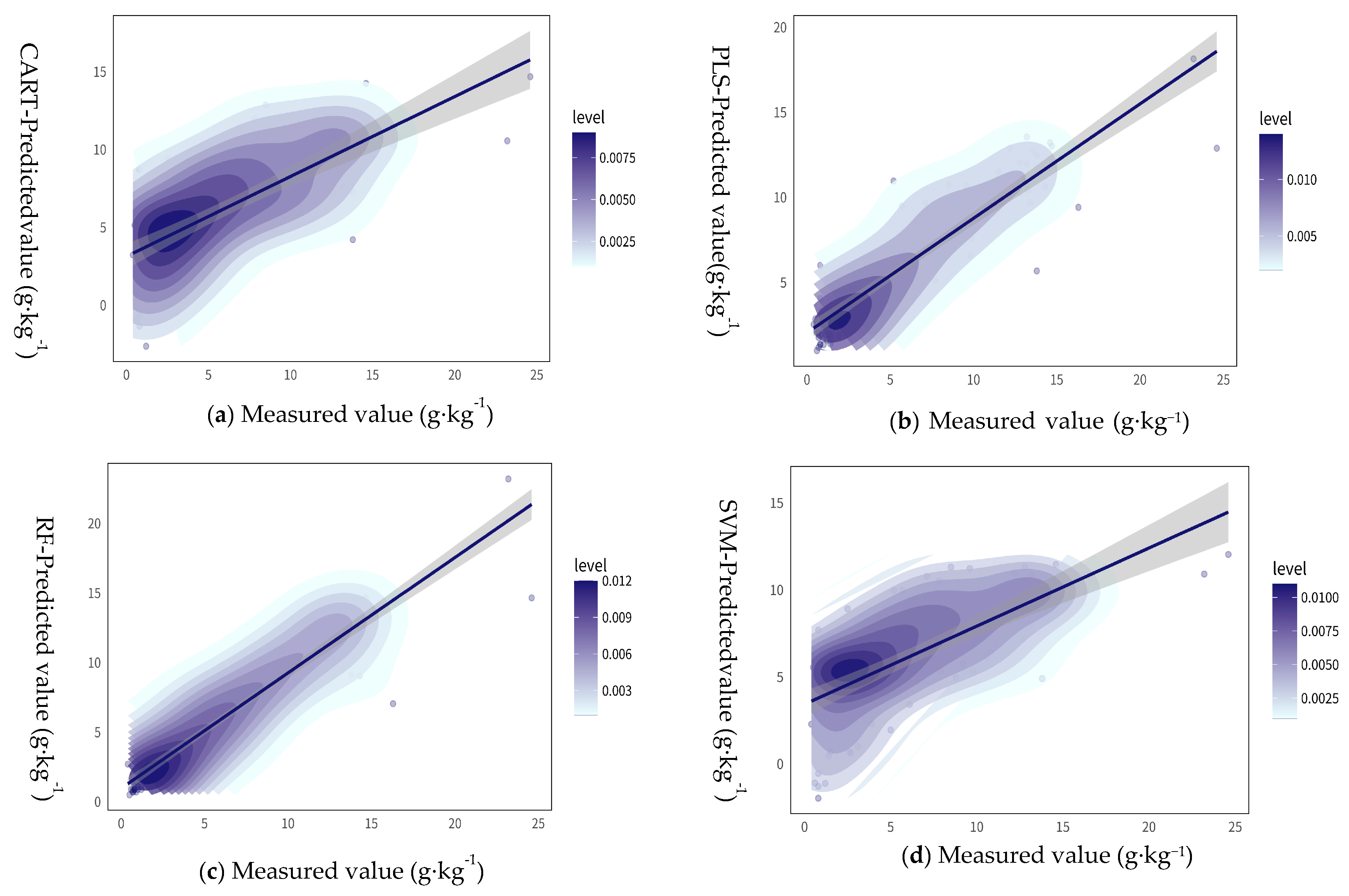
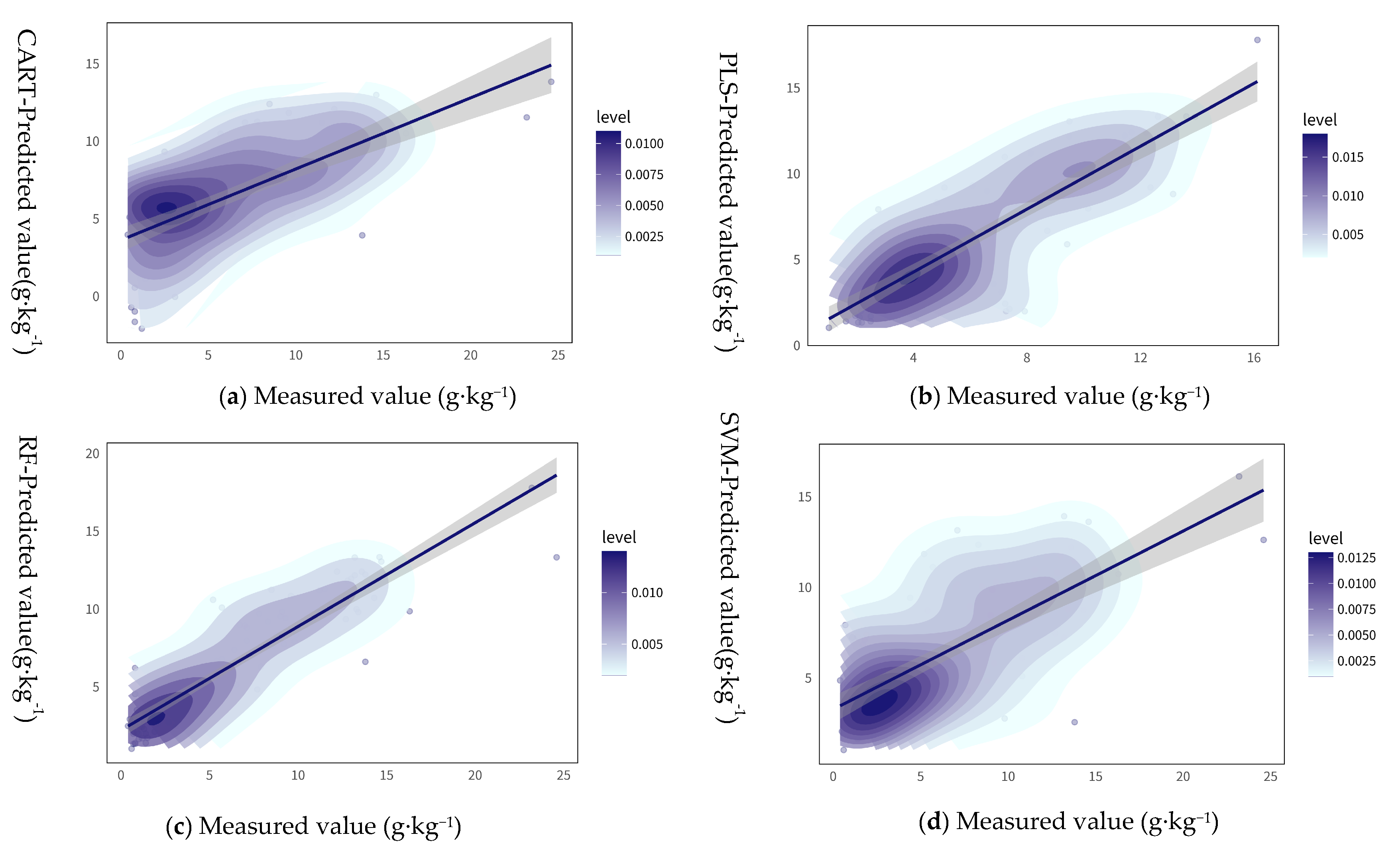
3.2. Model Accuracy Validation and Selection

Based on the 2002 2012, and 2022 datasets, the simulation accuracy of the different models was evaluated using the RMSE, MAE, and R2 metrics. Table 6 reports the results.
The RF regression model performed better at SSC (0–20 cm) (R2 = 0.723, RMSE 2.604 g·kg−1, MAE 1.95 g·kg−1) compared to SSC (20–40 cm) (R2 = 0.64, RMSE 3.62 g·kg−1, MAE 2.728 g·kg−1). Thus, the accuracy of the soil salinity monitoring model decreases with increasing depth. This indicates that the topsoil is more helpful for monitoring the changes in soil salinity at the same sampling time and location. The SVM regression model also performed better at SSC (0–20 cm) = (R2 = 0.459, RMSE of 3.829 g·kg−1, MAE of 3.494 g·kg−1) compared to SSC (20–40 cm) (R2 = 0.316, RMSE of 3.94 g·kg−1, MAE of 3.501 g·kg−1). This indicates the poor performance of the model with SVM. The model performs optimally with CART at SSC (0–20 cm) (R2 = 0.515, RMSE of 3.818 g·kg−1, MAE of 3.254 g·kg−1) and at SSC (20–40 cm) (R2 = 0.503, RMSE of 3.82 g·kg−1, MAE of 3.39 g·kg−1). Thus, the CART model performs consistently, with a similar accuracy performance at different depths. The PLS model performs optimally at SSC (0–20 cm) (R2 = 0.678, RMSE of 2.666 g·kg−1, MAE of 2.278 g·kg−1) and at SSC (20–40 cm) (R2 = 0.628, RMSE of 3.67 g·kg−1, MAE of 2.79 g·kg−1).
RF is observed to surpass SVM, CART, and PLS in terms of accuracy at SSC (0–20 cm) and SSC (20–40 cm) (Figure 5 and Figure 6). More specifically, the predicted RF soil salinity values provide the best fit with the measured soil salinity at both depths. Moreover, the PLS and CART models exhibit a strong ability to estimate soil salinity, while the SVM model performs poorly. Therefore, the RF model was chosen as the optimal monitoring model for soil salinization at the 0–20 cm and 20–40 cm soil depths and was employed to analyze the spatial and temporal changes in soil salinity in Bachu County for 2002, 2012, and 2022.

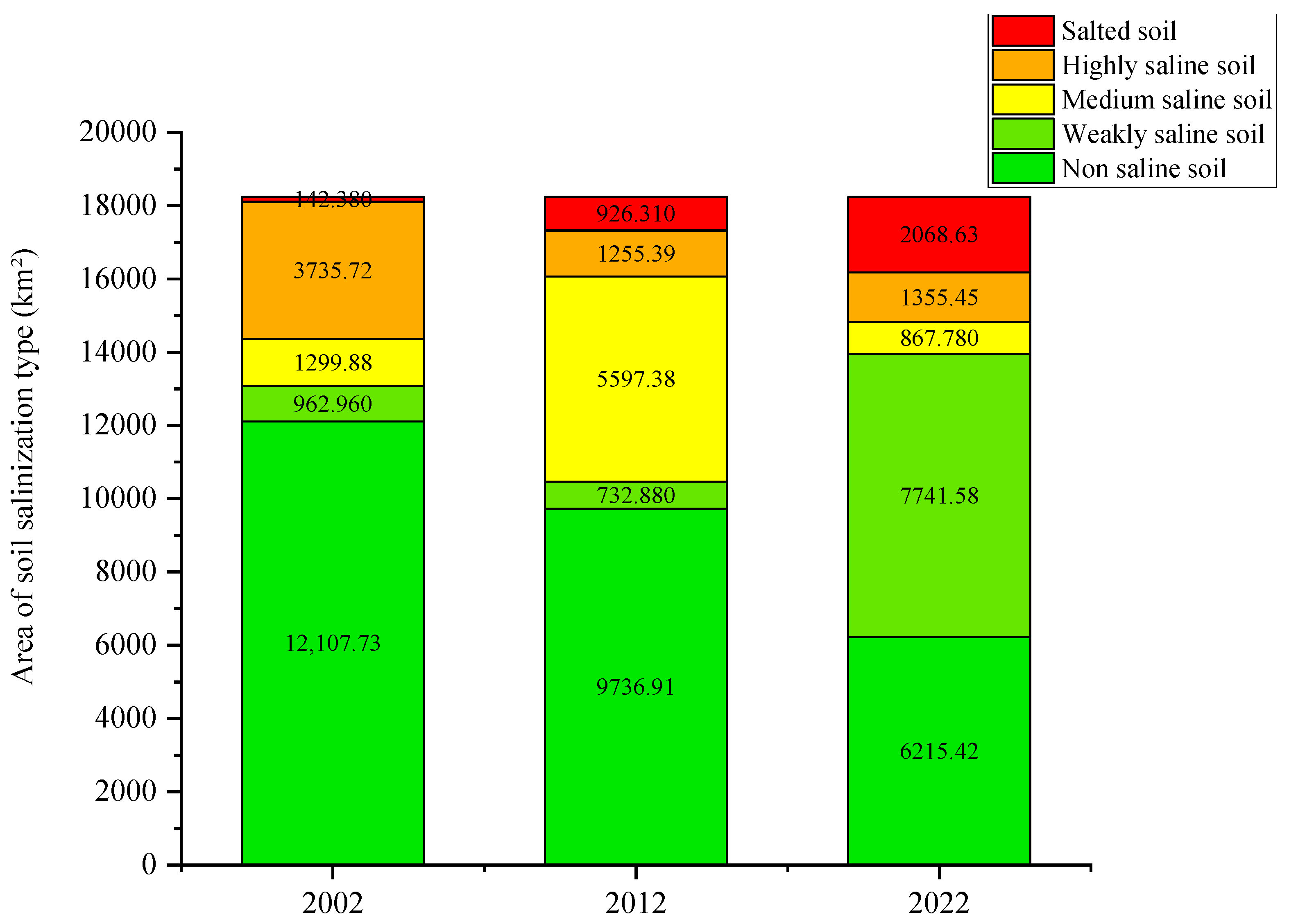
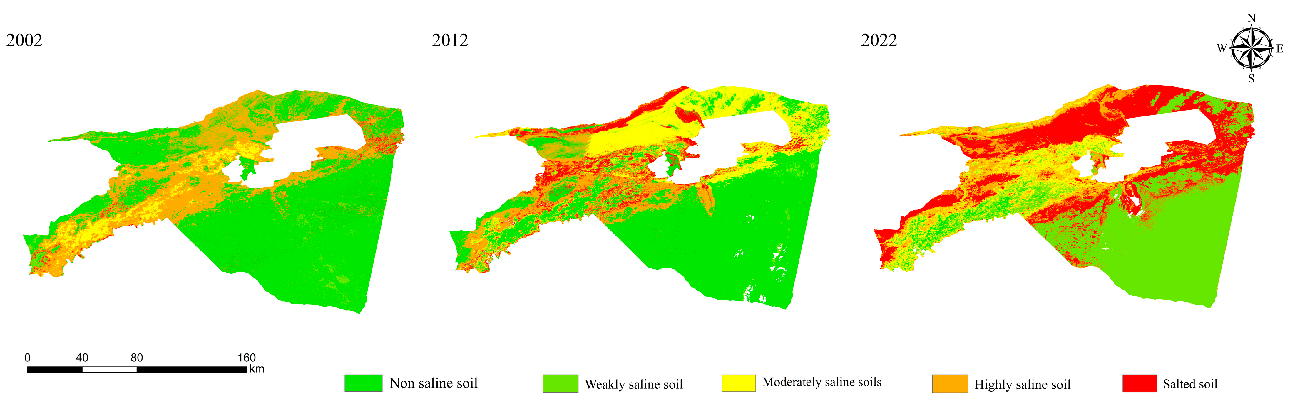
3.3. Spatial and Temporal Variability of Salinization in Bachu County

Soil salinization generally affects ecologically fragile and sensitive regions in inland arid areas. Previous research has investigated the correlation between ecological function reserves and changes in soil salinization [65]. We identified a correlation between the spatial distribution of soil salinization changes and the boundaries of ecological functional areas. This relationship can be attributed to the similarity in factors used to delineate ecological functional areas and predict soil salinization land classification. Thus, to clearly identify changes in soil salinization, we incorporate our results into the ecological functional area map of Bachu County. Figure 7 provides a detailed depiction of these changes.

3.3.1. Analysis of Spatial and Temporal Variations at the 0–20 cm Depth

We employed the Random Forest model (RFM) to estimate the soil salinity content of the study area at specific dates (April 2022, April 2012, and April 2002. The results were then used to determine the areas of different salinity types. Figure 8 reports a general improvement in soil salinity within the SSC (0–20 cm) depth from 2002 to 2022. The non-saline soil area decreased by 48.666% from 12,107.73 km2 to 6215.42 km2. Conversely, heavily salted soils decreased by 63.716% from 3735.72 km2 to 1355.45 km2, while saline soils increased significantly from 142.36 km2 to 2068.63 km2, denoting a rise of 1352.942%. The salinity was observed to vary across the years. This may be attributed to the increase in rainfall from year to year and the movement of salts to deeper layers of the soil. The increase in irrigation from human activities, the construction of drainage systems, and the introduction of soil conservation policies may play a role in the variation in salinity.
Table 7 reveals notable changes between 2002 and 2012, where non-saline soils converted to weakly saline, moderately saline, strongly saline, and saline soils, covering areas of 178.93 km2, 2586.03 km2, 355.94 km2, and 207.64 km2, respectively. These conversions predominantly occurred within ecological function areas, particularly in the oasis agriculture and desert riparian forest protection zones of the Yarkand River Plain, primarily extending toward the Tian grasslands on the southern mountain slopes. Weakly saline soils underwent conversions of 437.08 km2, 200.6 km2, 33.61 km2, and 40.24 km2 to non-saline, moderately saline, strongly saline, and saline soils, respectively. The majority of these changes occurred within the ecological function areas of oasis agriculture and desert riparian forest protection in the Yarkand River Plain, particularly targeting areas with a more delicate ecological environment. Strongly saline soils were converted into 316.087 km2, 84.89 km2, 2308.85 km2, and 386.43 km2 of non-saline, weakly saline, moderately saline, and saline soils, respectively. The majority of these transformations occurred within the ecologically sensitive areas of the Kashgar delta oasis, particularly affecting agricultural salinization, notably extending to the grasslands on the southern slopes of the Tianshan Mountains. Saline soils were converted to non-saline soils, weakly saline soils, moderately saline soils, and strongly saline soils with areas of 27.18 km2, 0.64 km2, 95.68 km2, and 11.89 km2, respectively. Most of these conversions occurred in the sensitive ecological function areas of the Kashgar delta oasis for agricultural salinization and the sensitive ecological function areas of the desert steppe for erosion in the western part of the southern slope of the Tianshan Mountains, with specific transfers to the more sensitive ecological environment of the grassland area on the south slope of Tianshan Mountain. Thus, fragile ecosystems are an influencing factor in the deepening soil salinization phenomenon. This may be linked to the reduction in vegetation cover, loss of biodiversity, and destruction of the soil protective layer associated with fragile ecosystems, thus increasing the risk of soil salt accumulation.
Table 8 illustrates the transformation of non-saline soils into weakly saline soils, moderately saline soils, strongly saline soils, and saline soils between 2012 and 2022, with conversion areas of 3541.94 km2, 146.98 km2, 62.48 km2, and 141.75 km2, respectively. The majority of these conversions occurred within the ecological functional area of the western flow desert landscape of the Taklamakan Desert, particularly toward the desert boundary. Weakly saline soils were converted into 218.78 km2, 161.08 km2, 77.74 km2, and 13.73 km2 of non-saline soils, moderately saline soils, strongly saline soils, and saline soils, respectively. The majority of these conversions occurred within the ecological functional areas of oasis agriculture in the Yarkand River Plain and the protection of riparian forests in the desert. More specifically, they were concentrated to the west of the Tarim Basin and the desert in the north. Moderately saline soils were converted into 789.58 km2, 2690.16 km2, 580.86 km2, and 1228.03 km2 of non-saline soils, weakly saline soils, strongly saline soils, and saline soils, respectively. The majority of these conversions occurred within the ecological functional areas of Yarkant River Plain Oasis Agriculture and Desert Riparian Forest Conservation, particularly in farmland adjacent to the desert. Strongly saline soils were transformed into non-saline, weakly saline, moderately saline, and saline soils with areas of 241.46 km2, 168.14 km2, 99.42 km2, and 470.35 km2, respectively. Most of these conversions occurred in the sensitive ecological functioning area of agricultural salinization in the Kashgar delta oasis, toward the farmland area boundaries close to the desert. Saline soils underwent conversions into non-saline soils, weakly saline soils, moderately saline soils, and strongly saline soils, covering areas of 121.84 km2, 79.79 km2, 151.54 km2, and 358.35 km2, respectively. The majority of these transformations occurred within the sensitive ecological function areas of agricultural salinization in the Kashgar delta oasis and the ecological function area of the western flowing desert landscape of the Taklamakan Desert. The results reveal that desertification contributes significantly to soil salinization, thus exacerbating its detrimental effects.
Figure 9 and Figure 10 shows that from 2002 to 2012, the main direction of the transfer of non-saline soils and strongly salinized soils was moderately salinized soils. Moreover, from 2012 to 2022, the main direction of the transfer of moderately salinized soils was weakly salinized soils. This change may be affected by several factors. For example, changes in precipitation may alter the distribution of soil salts, which consequently affects the transfer between salinized soil types. Changes in land use and management practices may also influence the distribution of soil salts. In addition, the upgrading of irrigation and drainage systems due to changes in human activities, policy improvements, and tendencies may impact soil salinity transfer. Although some areas may experience increased salinization, the observed transfer trends generally suggest an improvement in salinity.

3.3.2. Analysis of Spatial and Temporal Variations at the 20–40 cm Depth

Figure 11 reveals a general increase in soil salinization within the SSC (20–40 cm) depth from 2002 to 2022, accompanied by a significant reduction in the area of non-saline soil from 10,657.31 km2 to 207.59 km2. This denotes a decline of 98.052%. Despite a notable decrease of 54.746% in highly salinized soil from 5060 km2 to 2289.83 km2, there is a considerable rise in saline soils by 1715.145% from 288.90 km2 to 5243.88 km2. Thus, the prediction map depicts an overall increase in soil salinization at the SSC (20–40 cm) depth.
Table 9 shows that between 2002 and 2012, non-saline soils transformed into weakly saline soils (136.01 km2), moderately saline soils (1377.66 km2), strongly saline soils (1106.79 km2), and saline soils (412.99 km2), predominantly occurring in the ecological functional areas of oasis agriculture and desert riparian forest protection in the Yarkand River Plain. Notably, the shift toward the reservoir is observed primarily in areas of low human activity. Weakly saline soils underwent conversions totaling 1186.64 km2, 127.25 km2, 116.12 km2, and 12.19 km2 to non-saline soils, moderately saline soils, strongly saline soils, and saline soils, respectively. The majority of these conversions occurred within the ecological functional areas of oasis agriculture and desert riparian forest protection in the Yarkant River Plain. Moderately saline soils were converted to 373.05 km2, 200.29 km2, 31.24 km2, and 40.11 km2 of non-saline soils, weakly saline soils, strongly saline soils, and saline soils, respectively. The majority of these transformations occurred within the ecological functional areas of oasis agriculture in the Yarkand River Plain and the conservation zones of desert riparian forests, alongside the ecological functional area of the Western Mobile Desert Landscape in the Taklamakan Desert. Strongly saline soils underwent conversions to non-saline soils, weakly saline soils, moderately saline soils, and saline soils, covering areas of 529.88 km2, 349.18 km2, 2031.07 km2, and 1135.41 km2, respectively. The majority of these transformations occurred within the environmentally delicate regions affected by desert steppe erosion on the western part of the southern slope of the Tianshan Mountains, particularly in the ecologically sensitive and sparsely populated steppe areas on the southern slope of the Tianshan Mountains. Saline soils underwent conversions to non-saline soils, weakly saline soils, moderately saline soils, and strongly saline soils, covering areas of 49.47 km2, 1.26 km2, 130.19 km2, and 85.04 km2, respectively. The majority of these transformations occurred within the agro-salinity-sensitive eco-functional zones of the Kashmir Delta oasis, particularly targeting the agro-ecological zones with higher anthropogenic activities. The results indicate that soil salinization occurs frequently in areas of human activity and varies with the type of activity, including irrigation, land reclamation, overgrazing, and fertilizer and pesticide use. These activities lead to the accumulation and build-up of salts in the soil, which in turn exacerbate the degree of soil salinization.
Table 10 reveals substantial transformations of non-saline soils into weakly saline soils (7245.48 km2), moderately saline soils (223.38 km2), strongly saline soils (353.55 km2) and saline soils (1771.51 km2) between 2012 and 2022. These conversions predominantly occurred within the ecological functional areas of oasis agriculture and desert riparian forest protection in the Yarkant River Plain and the Western Taklamakan Desert Mobile Desert Landscape Ecological Functional Area. Notably, these changes in soil often occurred in regions with limited human intervention, such as the desert in the northern Tarim Basin. Weakly saline soils were converted to 40.78 km2, 230.27 km2, 45.22 km2, and 5.26 km2 of non-saline soils, moderately saline soils, strongly saline soils, and saline soils, respectively. These exchanges predominantly occurred within the ecological functional areas of Yarkand River Plain oasis agriculture and desert riparian forest protection. Moderately saline soils underwent conversions of 22.93 km2, 454.41 km2, 392.75 km2, and 2462.10 km2 to non-saline soils, weakly saline soils, strongly saline soils, and saline soils, respectively. The majority of these changes occurred within the ecological function areas of oasis agriculture and desert riparian forest protection in the Yarkand River Plain, as well as the sensitive ecological function areas affected by desert steppe erosion on the western part of the southern slope of the Tianshan Mountains. Strongly saline soils were converted into non-saline soils, weakly saline soils, moderately saline soils, and saline soils, covering areas of 3.35 km2, 81.27 km2, 599.63 km2, and 804.23 km2, respectively. The majority of these conversions occurred in the Kashgar delta oasis, a sensitive ecological area prone to agricultural salinization, in areas affected by desert steppe soil erosion on the western part of the southern slope of the Tianshan Mountains, and in the western part of the Taklamakan Desert Mobile Desert Landscape Ecological Functional Area. In particular, there was a notable transfer to the grassland area on the southern slope of the Tianshan Mountains, characterized by lower human activity levels. Saline soils underwent conversions to non-saline, weakly saline, moderately saline, and strongly saline soils, covering areas of 5.31 km2, 118.93 km2, 638.33 km2, and 653.48 km2, respectively. The majority of these conversions occurred in the ecologically sensitive areas of the Kashgar delta oasis, affected by agricultural salinization, and in the ecological function area of the western mobile desert landscape of the Taklamakan Desert. The above analysis highlights the exacerbation of salinization hazards in mountainous and Gobi areas over time, despite minimal human activity.
Figure 12 and Figure 13 depicts the transfer of soil salinity types in the SSC (20–40 cm) depth, revealing the dominant trends in soil transfer dynamics from 2002 to 2012. Non-saline soils generally transitioned to moderately saline soils, while weakly saline soils shifted toward non-saline soils. Moderately saline soils, in turn, transitioned to weakly saline soils. In addition, highly saline soils mainly transformed into moderately saline soils and saline soils, with saline soils exhibiting a primary transition to moderately saline soils. Conversely, between 2012 and 2022, non-saline and moderately saline soils primarily transitioned to saline soils. Similarly, highly saline soils predominantly transformed into saline soils. This indicates that while there was a reduction in deep-soil salinity before 2012, deep-soil salinity intensified, exacerbating overall salinization by 2022.

3.4. Validation of Model Prediction Classification Errors

To validate the accuracy of the soil salinity model classification, we compared the 50 validation sites sampled in 2022 with the soil salinity classification map. This comparison revealed discrepancies in soil salinity types at five sample sites when compared to the measured salinity sample sites: The dataset comprises 10 samples from each soil type (non-saline, weakly saline, moderately saline, highly saline, and saline soils). These 50 measured sample points were overlaid onto the soil salinity classification map to assess the accuracy of soil salinity categorization. Verification confirms the consistency between the model classifications and actual soil salinity. After comparing the four models, it was observed that the RF model exhibited the highest predictive performance in the radargrams at SSC (0–20 cm) and SSC (20–40 cm). PLS demonstrated a slightly lower performance but still maintained an accuracy above 50%, while CART and SVM exhibited inferior performances. Moreover, the classifications were generally more accurate for SSC (0–20 cm) compared to SSC (20–40 cm). The predictive maps derived at the two depths exhibited higher accuracy in predicting non-saline and weakly saline soils and a lower accuracy in predicting saline soils (Figure 14).

4. Discussion

Soil salinization has become a global problem. To quickly and accurately evaluate the impacts of soil salinization on regional ecological badlands and agricultural farming, this study proposes a model to monitor the changes and transfer of soil-salinized land in Bachu County based on the GEE cloud computing platform. The proposed model combines numerous indices and machine learning models. The measured soil salinization is correlated with six types of indices related to soil salinization and six optimal factors are selected. Four predictive regression models were constructed by combining the six optimal factors. After evaluating the prediction accuracy and error of the models, the optimal model RF was selected to predict the change of soil salinization at different depths, and the data from three years were extracted to analyze the spatial and temporal changes of salinization in Bachu County over the past 20 years. The SVM model is unable to adequately capture the variability of soil salinity due to the complex relationship between the data features. The CART model may not be able to capture the complex variability patterns of soil salinity due to its simple partitioning rule. The PLS model may not be able to adequately fit soil salinity due to the assumed linear relationship between the data features.

4.1. Selection of Model Indices

We selected 31 factors for correlation analysis with surface soil salinity at two depths. To prevent multicollinearity among similar indices, one index was selected from each of the six index types. The selected indices, NDVI, SI3, RED, ELEVATION, ET, and SDI, align with those adopted in previous research [14]. The correlation between the six indices is optimal at the depths of SSC (0–20 cm) and SSC (20–40 cm). Among the vegetation indices, the NDVI has the highest correlation with soil salinity. This is likely to be attributed to the high sensitivity of the NDVI to the physiological and ecological characteristics of vegetation, allowing it to reflect the growth status of vegetation more accurately, including the influence of soil salinity. SI3, on the other hand, has a higher relevance among the salinity indices as it is obtained by multiplying the reflectance of the green and red light bands. This accurately captures the effect of soil salinity on vegetation as the green and red light bands are usually better reflectors of vegetation growth and soil surface cover. RED has the highest correlation with soil salinity among single bands as soil areas containing high salinity tend to be lighter in color, while low-salinity soils are darker. The red band is typically more sensitive to color changes in soils and therefore better able to differentiate between soils with different salinity levels compared to other bands. ELEVATION represents the elevation of the land surface. Topography has an important effect on the distribution of soil salts, which may explain its strong correlation with soil salinity. ET is a composite index of the evapotranspiration of soil moisture and the transpiration of vegetation. It is closely related to the distribution of soil salts, which may explain its high correlation with soil salinity. The SDI is often used to reflect the moisture status of the soil, particularly the degree of wetness or dryness of the surface soil. Highly saline soils may lead to the rapid evaporation of soil water, thus making the soil more susceptible to drying, which may be less relevant than other composite indices.

4.2. Validation of the Model Accuracy and Classification Error

The model performance accuracy was higher at the SSC (0–20 cm) depth compared to the SSC (20–40 cm) depth. The R2 values of the four models (RF, SVM, CART, and PLS) were 0.723, 0.459, 0.515, and 0.678, respectively, with the RF regression model exhibiting the highest performance accuracy. This is consistent with the findings of previous research [66,67]. The model error is lower for the SSC (0–20 cm) depth in the classification map, indicating that the topsoil prediction model performs better than the deep-soil prediction model.
The RF regression model outperformed the other models in terms of accuracy at the two depths of SSC (0–20 cm) and SSC (20–40 cm), with R2 values of 0.723 and 0.64, respectively. For SSC (0–20 cm), the RF model had an RMSE of 2.604 g·kg−1 and MAE of 1.95 g·kg−1, while for SSC (20–40 cm), the values were RMSE = 3.62 g·kg−1 and MAE = 2.728 g·kg−1. The RF regression model exhibited the lowest error in the classification map across the two depths in the classification model. This underscores the high accuracy of the RF regression model, which integrates multiple indices, for the monitoring of soil salinization.

4.3. Analysis of Spatial and Temporal Changes in Soil Salinization and Their Influencing Factors in Bachu County

Between 2002 and 2012, there was a notable transition from non-saline and saline soils to moderately saline soils. This shift from non-saline soils can be attributed to improper irrigation practices, leading to extensive soil salinization in cultivated areas. In addition, the fragile ecological environment exacerbated the extent of soil salinization. The transformation of saline soils into moderately saline soils is attributed to the increased awareness of ecological preservation and the implementation of national policies aimed at desertification prevention and sand stabilization. Consequently, there has been a concerted effort to remediate salinized land along the fringes of vast desert expanses.
Substantial quantities of non-saline and moderately saline soils transitioned to weakly saline soils between 2012 and 2022. The majority of these shifts in non-saline soils were observed in agricultural areas and the west–central mountain ranges, indicating the influence of human activities and topography on soil salinization. Salinization has also shifted within the same area, indicating that human intervention, such as the adoption of scientific irrigation practices and growing environmental consciousness, has somewhat mitigated salinization. This demonstrates that human activities can have adverse and beneficial impacts on soil salinization.
Soil salinity varied across the two depths. SCC (0–20 cm) exhibited weaker salinization compared to SCC (20–40 cm) due to the downward leaching of salts from the topsoil in irrigated farmlands. In terms of accuracy at different depths, the correlation between water-soluble salts and numerous indices (e.g., spectral indices) decreased as the sampling depth increased. This is due to the relatively low sensitivity of the bottom layer of the soil to spectral bands, as remotely sensed spectral information can only represent surface information, which is in line with the results of previous research [68].

4.4. Future Prospects and Challenges

We performed spatio-temporal analysis for three periods and at two depths, making great progress in the research field. However, this study still has some shortcomings. For example, although the spatio-temporal analysis was combined with ecological reserves, we did not explore the impacts of soil salinization on land use types. In addition, due to the limited sample point data, only the area of Bachu County was studied, with a focus on arid areas. Thus, the applicability of the model under a larger scope requires further examination, with the inclusion of other areas. Moreover, GEE-based modeling is low-cost, simple, and improves the monitoring speed compared with other satellite remote sensing monitoring methods. However, its accuracy may be lower in small-scale areas compared with accurate low-altitude remote sensing approaches. The presence of cloud cover also limits the monitoring of the GEE remote sensing platform, while low-altitude remote sensing platforms such as aerial vehicles or unmanned aerial vehicles (UAVs) do not have this limitation. Moreover, we did not test the model accuracy for different years at the same depth, nor did we test the model stability. The GEE platform also lacks several common machine learning algorithms. For example, BP neural networks are robust predictive regression models, yet we were unable to find related code and data on GEE.

5. Conclusions

In this study, the RF, SVM, CART, and PLS models were used to assess the accuracy of machine learning and empirical models. These models were combined with various indices to develop two models for estimating soil salinity at different depths. The model accuracy was subsequently validated. Based on the results, the following conclusions were determined:
NDVI, SI3, RED, ELEVATION, ET, and SDI exhibited the highest correlations with soil salinity measurements. The four models were ranked in terms of accuracy as follows: RF > PLS > CART > SVM. Although all four models exhibited good accuracy, the RF model was more accurate, while the PLS model was more stable at the two depths.
The accuracy of the models was affected by the soil depth, as evidenced by the correlation between various indicators and soil salinity measurements at different depths. Categorical error plot analysis revealed that the surface soil at the SCC (0–20 cm) depth had a stronger correlation with the indicators, resulting in a better model performance.
The prediction model effectively captured the spatial and temporal changes in soil salinization in Bachu County. The high-salinity areas were mainly distributed in anthropogenic-intensive areas and mountainous areas. The salinization degree of the surface (0–20 cm) and deep (20–40 cm) soils decreased between 2002 and 2012. During 2012–2022, soil salinization in the surface layer (0–20 cm) of sandy land decreased, while soil salinization in the deep layer (20–40 cm) of sandy land increased.

Author Contributions

Conceptualization, Y.Z. and H.W.; methodology, Y.F.; software, Y.K.; validation, Y.Z., H.W. and Y.F.; formal analysis, H.W.; investigation, S.W. and F.H.; resources, Z.L.; data curation, Y.Z.; writing—original draft preparation, Y.Z.; writing—review and editing, Y.Z.; visualization, Y.K.; supervision, Y.K.; project administration, H.W.; funding acquisition, Y.F. All authors have read and agreed to the published version of the manuscript.

Funding

Integration and Demonstration of Technical Models for Soil Improvement and Capacity Enhancement in Northwest Saline Soil Area 2023YFD1901503.

Institutional Review Board Statement

Not applicable.

Data Availability Statement

The data presented in this study are available upon request from the corresponding author.

Conflicts of Interest

The authors declare no conflicts of interest.

References

  1. Li, J.; Pu, L.; Han, M.; Zhu, M.; Zhang, R.; Xiang, Y. Soil salinization research in China: Advances and prospects. J. Geogr. Sci. 2014, 24, 943–960. [Google Scholar] [CrossRef]
  2. Wang, H.; Jia, G. Satellite-based monitoring of decadal soil salinization and climate effects in a semi-arid region of China. Adv. Atmos. Sci. 2012, 29, 1089–1099. [Google Scholar] [CrossRef]
  3. Bouksila, F.; Bahri, A.; Berndtsson, R.; Persson, M.; Rozema, J.; Van der Zee, S.E. Assessment of soil salinization risks under irrigation with brackish water in semiarid Tunisia. Environ. Exp. Bot. 2013, 92, 176–185. [Google Scholar] [CrossRef]
  4. Cañedo-Argüelles, M.; Kefford, B.J.; Piscart, C.; Prat, N.; Schäfer, R.B.; Schulz, C.-J. Salinisation of rivers: An urgent ecological issue. Environ. Pollut. 2013, 173, 157–167. [Google Scholar] [CrossRef] [PubMed]
  5. Tanji, K.K. Nature and extent of agricultural salinity. Agric. Salin. Assess. Manag. 1990, 71–92. Available online: https://www.encyclopedie-environnement.org/zh/zoom/land-salinization/ (accessed on 9 April 2024).
  6. Panah, A.; Kazem, S.; McKenzie, N. Status of the world’s soil resources main report. Available online: http://www.alice.cnptia.embrapa.br/alice/handle/doc/1034770 (accessed on 9 April 2024).
  7. Scudiero, E.; Skaggs, T.H.; Corwin, D.L. Simplifying field-scale assessment of spatiotemporal changes of soil salinity. Sci. Total Environ. 2017, 587, 273–281. [Google Scholar] [CrossRef] [PubMed]
  8. Dent, D.; Young, A. Soil Survey and Land Evaluation; George Allen & Unwin: Sydney, NSW, Australia, 1981. [Google Scholar]
  9. Nanni, M.R.; Demattê, J.A.M. Spectral reflectance methodology in comparison to traditional soil analysis. Soil Sci. Soc. Am. J. 2006, 70, 393–407. [Google Scholar] [CrossRef]
  10. Dehaan, R.; Taylor, G. Field-derived spectra of salinized soils and vegetation as indicators of irrigation-induced soil salinization. Remote Sens. Environ. 2002, 80, 406–417. [Google Scholar] [CrossRef]
  11. Asfaw, E.; Suryabhagavan, K.; Argaw, M. Soil salinity modeling and mapping using remote sensing and GIS: The case of Wonji sugar cane irrigation farm, Ethiopia. J. Saudi Soc. Agric. Sci. 2018, 17, 250–258. [Google Scholar] [CrossRef]
  12. Gorji, T.; Sertel, E.; Tanik, A. Monitoring soil salinity via remote sensing technology under data scarce conditions: A case study from Turkey. Ecol. Indic. 2017, 74, 384–391. [Google Scholar] [CrossRef]
  13. Mougenot, B.; Pouget, M.; Epema, G. Remote sensing of salt affected soils. Remote Sens. Rev. 1993, 7, 241–259. [Google Scholar] [CrossRef]
  14. Wang, Z.; Zhang, F.; Zhang, X.; Chan, N.W.; Ariken, M.; Zhou, X.; Wang, Y. Regional suitability prediction of soil salinization based on remote-sensing derivatives and optimal spectral index. Sci. Total Environ. 2021, 775, 145807. [Google Scholar] [CrossRef]
  15. Zhang, Z.; Fan, Y.; Zhang, A.; Jiao, Z. Baseline-Based Soil Salinity Index (BSSI): A Novel Remote Sensing Monitoring Method of Soil Salinization. IEEE J. Sel. Top. Appl. Earth Obs. Remote Sens. 2022, 16, 202–214. [Google Scholar] [CrossRef]
  16. Ding, J.-L.; Wu, M.-C.; Liu, H.-X.; Li, Z.-G. Study on the soil salinization monitoring based on synthetical hyperspectral index. Spectrosc. Spectr. Anal. 2012, 32, 1918–1922. [Google Scholar]
  17. Triki Fourati, H.; Bouaziz, M.; Benzina, M.; Bouaziz, S. Detection of terrain indices related to soil salinity and mapping salt-affected soils using remote sensing and geostatistical techniques. Environ. Monit. Assess. 2017, 189, 177. [Google Scholar] [CrossRef] [PubMed]
  18. El Harti, A.; Lhissou, R.; Chokmani, K.; Ouzemou, J.-E.; Hassouna, M.; Bachaoui, E.M.; El Ghmari, A. Spatiotemporal monitoring of soil salinization in irrigated Tadla Plain (Morocco) using satellite spectral indices. Int. J. Appl. Earth Obs. Geoinf. 2016, 50, 64–73. [Google Scholar] [CrossRef]
  19. Wu, D.; Jia, K.; Zhang, X.; Zhang, J.; Abd El-Hamid, H.T. Remote sensing inversion for simulation of soil salinization based on hyperspectral data and ground analysis in Yinchuan, China. Nat. Resour. Res. 2021, 30, 4641–4656. [Google Scholar] [CrossRef]
  20. Shi, H.; Hellwich, O.; Luo, G.; Chen, C.; He, H.; Ochege, F.U.; Van de Voorde, T.; Kurban, A.; De Maeyer, P. A global meta-analysis of soil salinity prediction integrating satellite remote sensing, soil sampling, and machine learning. IEEE Trans. Geosci. Remote Sens. 2021, 60, 4505815. [Google Scholar] [CrossRef]
  21. Jiang, H.; Shu, H. Optical remote-sensing data based research on detecting soil salinity at different depth in an arid-area oasis, Xinjiang, China. Earth Sci. Inform. 2019, 12, 43–56. [Google Scholar] [CrossRef]
  22. Wang, Q.; Li, P.; Chen, X. Retrieval of soil salt content from an integrated approach of combining inversed reflectance model and regressions: An experimental study. IEEE Trans. Geosci. Remote Sens. 2012, 50, 3950–3957. [Google Scholar] [CrossRef]
  23. Barbouchi, M.; Abdelfattah, R.; Chokmani, K.; Aissa, N.B.; Lhissou, R.; El Harti, A. Soil salinity characterization using polarimetric InSAR coherence: Case studies in Tunisia and Morocco. IEEE J. Sel. Top. Appl. Earth Obs. Remote Sens. 2014, 8, 3823–3832. [Google Scholar] [CrossRef]
  24. Zhang, Q.; Li, L.; Sun, R.; Zhu, D.; Zhang, C.; Chen, Q. Retrieval of the soil salinity from Sentinel-1 Dual-Polarized SAR data based on deep neural network regression. IEEE Geosci. Remote Sens. Lett. 2020, 19, 4006905. [Google Scholar] [CrossRef]
  25. Tian, A.; Fu, C.; Yau, H.-T.; Su, X.-Y.; Xiong, H. A new methodology of soil salinization degree classification by probability neural network model based on centroid of fractional lorenz chaos self-synchronization error dynamics. IEEE Trans. Geosci. Remote Sens. 2019, 58, 799–810. [Google Scholar] [CrossRef]
  26. Ma, S.; He, B.; Ge, X.; Luo, X. Spatial prediction of soil salinity based on the Google Earth Engine platform with multitemporal synthetic remote sensing images. Ecol. Inform. 2023, 75, 102111. [Google Scholar] [CrossRef]
  27. Dong, J.; Xiao, X.; Menarguez, M.A.; Zhang, G.; Qin, Y.; Thau, D.; Biradar, C.; Moore III, B. Mapping paddy rice planting area in northeastern Asia with Landsat 8 images, phenology-based algorithm and Google Earth Engine. Remote Sens. Environ. 2016, 185, 142–154. [Google Scholar] [CrossRef] [PubMed]
  28. Xiong, J.; Thenkabail, P.S.; Tilton, J.C.; Gumma, M.K.; Teluguntla, P.; Oliphant, A.; Congalton, R.G.; Yadav, K.; Gorelick, N. Nominal 30-m cropland extent map of continental Africa by integrating pixel-based and object-based algorithms using Sentinel-2 and Landsat-8 data on Google Earth Engine. Remote Sens. 2017, 9, 1065. [Google Scholar] [CrossRef]
  29. Parastatidis, D.; Mitraka, Z.; Chrysoulakis, N.; Abrams, M. Online global land surface temperature estimation from Landsat. Remote Sens. 2017, 9, 1208. [Google Scholar] [CrossRef]
  30. Brovelli, M.A.; Sun, Y.; Yordanov, V. Monitoring forest change in the amazon using multi-temporal remote sensing data and machine learning classification on Google Earth Engine. ISPRS Int. J. Geo-Inf. 2020, 9, 580. [Google Scholar] [CrossRef]
  31. Zhang, W.; Cao, L.; Yu, S.; Zhou, X. Study on Surface and Internal Humidity of Dunes in the Southwestern Margin of the Taklimakan Desert. In Proceedings of the 2nd International Conference on Green Energy, Environment and Sustainable Development (GEESD2021), Shanghai, China, 26–27 June 2021; p. 462. [Google Scholar]
  32. Mamat, A.; Halik, Ü.; Rouzi, A. Variations of ecosystem service value in response to land-use change in the Kashgar Region, Northwest China. Sustainability 2018, 10, 200. [Google Scholar] [CrossRef]
  33. Jiang, P. Soil Improvement and Fertilization; Xinjiang People’s Publishing House: Urumqi, China, 2012; pp. 121–148. [Google Scholar]
  34. Luo, C.; Zhang, X.; Meng, X.; Zhu, H.; Ni, C.; Chen, M.; Liu, H. Regional mapping of soil organic matter content using multitemporal synthetic Landsat 8 images in Google Earth Engine. Catena 2022, 209, 105842. [Google Scholar] [CrossRef]
  35. Zhang, J.; Zhang, Z.; Chen, J.; Chen, H.; Jin, J.; Han, J.; Wang, X.; Song, Z.; Wei, G. Estimating soil salinity with different fractional vegetation cover using remote sensing. Land Degrad. Dev. 2021, 32, 597–612. [Google Scholar] [CrossRef]
  36. Taghizadeh-Mehrjardi, R.; Minasny, B.; Sarmadian, F.; Malone, B. Digital mapping of soil salinity in Ardakan region, central Iran. Geoderma 2014, 213, 15–28. [Google Scholar] [CrossRef]
  37. Mejia-Cabrera, H.I.; Vilchez, D.; Tuesta-Monteza, V.; Forero, M.G. Soil salinity estimation of sparse vegetation based on multispectral image processing and machine learning. In Proceedings of the Applications of Digital Image Processing XLIII, Online, 24 August–4 September 2020; pp. 81–90. [Google Scholar]
  38. Hongyan, C.; Gengxing, Z.; Jingchun, C.; Ruiyan, W.; Mingxiu, G. Remote sensing inversion of saline soil salinity based on modified vegetation index in estuary area of Yellow River. Trans. Chin. Soc. Agric. Eng. 2015, 31, 107–114. [Google Scholar]
  39. Song, B.; Park, K. Detection of aquatic plants using multispectral UAV imagery and vegetation index. Remote Sens. 2020, 12, 387. [Google Scholar] [CrossRef]
  40. Rondeaux, G.; Steven, M.; Baret, F. Optimization of soil-adjusted vegetation indices. Remote Sens. Environ. 1996, 55, 95–107. [Google Scholar] [CrossRef]
  41. Azabdaftari, A.; Sunar, F. Soil salinity mapping using multitemporal Landsat data. Int. Arch. Photogramm. Remote Sens. Spat. Inf. Sci. 2016, 41, 3–9. [Google Scholar] [CrossRef]
  42. Ding, J.; Yu, D. Monitoring and evaluating spatial variability of soil salinity in dry and wet seasons in the Werigan–Kuqa Oasis, China, using remote sensing and electromagnetic induction instruments. Geoderma 2014, 235, 316–322. [Google Scholar] [CrossRef]
  43. Abbas, A.; Khan, S. Using remote sensing techniques for appraisal of irrigated soil salinity. In Proceedings of the International Congress on Modelling and Simulation (MODSIM), Brisbane, Australia, 10–12 December 2007; pp. 2632–2638. [Google Scholar]
  44. Nicolas, H.; Walter, C. Detecting salinity hazards within a semiarid context by means of combining soil and remote-sensing data. Geoderma 2006, 134, 217–230. [Google Scholar]
  45. Bannari, A.; Guedon, A.; El-Harti, A.; Cherkaoui, F.; El-Ghmari, A. Characterization of slightly and moderately saline and sodic soils in irrigated agricultural land using simulated data of advanced land imaging (EO-1) sensor. Commun. Soil Sci. Plant Anal. 2008, 39, 2795–2811. [Google Scholar] [CrossRef]
  46. Allbed, A.; Kumar, L.; Aldakheel, Y.Y. Assessing soil salinity using soil salinity and vegetation indices derived from IKONOS high-spatial resolution imageries: Applications in a date palm dominated region. Geoderma 2014, 230, 1–8. [Google Scholar] [CrossRef]
  47. Allbed, A.; Kumar, L.; Sinha, P. Mapping and modelling spatial variation in soil salinity in the Al Hassa Oasis based on remote sensing indicators and regression techniques. Remote Sens. 2014, 6, 1137–1157. [Google Scholar] [CrossRef]
  48. Al-Khaier, F. Soil salinity detection using satellite remote sensing. 2003. Available online: https://webapps.itc.utwente.nl/librarywww/papers_2003/msc/wrem/khaier.pdf (accessed on 9 April 2024).
  49. Tripathi, N.; Rai, B.K.; Dwivedi, P. Spatial modeling of soil alkalinity in GIS environment using IRS data. In Proceedings of the Proceedings of the 18th Asian Conference on Remote Sensing, Kuala Lumpur, Malaysia, 20–24 October 1997; pp. 20–24. [Google Scholar]
  50. Khan, N.M.; Rastoskuev, V.V.; Shalina, E.V.; Sato, Y. Mapping salt-affected soils using remote sensing indicators—A simple approach with the use of GIS IDRISI. In Proceedings of the 22nd Asian Conference on Remote Sensing, Singapore, 5–9 November 2001. [Google Scholar]
  51. Liu, J.; Zhang, L.; Dong, T.; Wang, J.; Fan, Y.; Wu, H.; Geng, Q.; Yang, Q.; Zhang, Z. The applicability of remote sensing models of soil salinization based on feature space. Sustainability 2021, 13, 13711. [Google Scholar] [CrossRef]
  52. Wu, Z.; Lei, S.; Bian, Z.; Huang, J.; Zhang, Y. Study of the desertification index based on the albedo-MSAVI feature space for semi-arid steppe region. Environ. Earth Sci. 2019, 78, 232. [Google Scholar] [CrossRef]
  53. Guo, B.; Yang, F.; Fan, Y.; Han, B.; Chen, S.; Yang, W. Dynamic monitoring of soil salinization in Yellow River Delta utilizing MSAVI–SI feature space models with Landsat images. Environ. Earth Sci. 2019, 78, 308. [Google Scholar] [CrossRef]
  54. Liang, S. Narrowband to broadband conversions of land surface albedo I: Algorithms. Remote Sens. Environ. 2001, 76, 213–238. [Google Scholar] [CrossRef]
  55. Behrens, T.; Zhu, A.-X.; Schmidt, K.; Scholten, T. Multi-scale digital terrain analysis and feature selection for digital soil mapping. Geoderma 2010, 155, 175–185. [Google Scholar] [CrossRef]
  56. Shokri-Kuehni, S.M.; Rad, M.N.; Webb, C.; Shokri, N. Impact of type of salt and ambient conditions on saline water evaporation from porous media. Adv. Water Resour. 2017, 105, 154–161. [Google Scholar] [CrossRef]
  57. Pang, G.; Wang, T.; Liao, J.; Li, S. Quantitative Model Based on Field-Derived Spectral Characteristics to Estimate Soil Salinity in Minqin County, China. Soil Sci. Soc. Am. J. 2014, 78, 546–555. [Google Scholar] [CrossRef]
  58. Guan, X.; Wang, S.; Gao, Z.; Lv, Y. Dynamic prediction of soil salinization in an irrigation district based on the support vector machine. Math. Comput. Model. 2013, 58, 719–724. [Google Scholar] [CrossRef]
  59. Aksoy, S.; Yildirim, A.; Gorji, T.; Hamzehpour, N.; Tanik, A.; Sertel, E. Assessing the performance of machine learning algorithms for soil salinity mapping in Google Earth Engine platform using Sentinel-2A and Landsat-8 OLI data. Adv. Space Res. 2022, 69, 1072–1086. [Google Scholar] [CrossRef]
  60. Kabiraj, S.; Jayanthi, M.; Vijayakumar, S.; Duraisamy, M. Comparative assessment of satellite images spectral characteristics in identifying the different levels of soil salinization using machine learning techniques in Google Earth Engine. Earth Sci. Inform. 2022, 15, 2275–2288. [Google Scholar] [CrossRef]
  61. Esposito Vinzi, V.; Russolillo, G. Partial least squares algorithms and methods. Wiley Interdiscip. Rev. Comput. Stat. 2013, 5, 1–19. [Google Scholar] [CrossRef]
  62. Awad, M. Google Earth Engine (GEE) cloud computing based crop classification using radar, optical images and Support Vector Machine Algorithm (SVM). In Proceedings of the 2021 IEEE 3rd International Multidisciplinary Conference on Engineering Technology (IMCET), Beirut, Lebanon, 8–10 December 2021; pp. 71–76. [Google Scholar]
  63. Lee, S.K. On classification and regression trees for multiple responses and its application. J. Classif. 2006, 23, 123–141. [Google Scholar] [CrossRef]
  64. Dhillon, M.S.; Dahms, T.; Kuebert-Flock, C.; Rummler, T.; Arnault, J.; Steffan-Dewenter, I.; Ullmann, T. Integrating random forest and crop modeling improves the crop yield prediction of winter wheat and oil seed rape. Front. Remote Sens. 2023, 3, 1010978. [Google Scholar] [CrossRef]
  65. Sun, Q.; Sun, J.; Baidurela, A.; Li, L.; Hu, X.; Song, T. Ecological landscape pattern changes and security from 1990 to 2021 in Ebinur Lake Wetland Reserve, China. Ecol. Indic. 2022, 145, 109648. [Google Scholar] [CrossRef]
  66. Wang, N.; Xue, J.; Peng, J.; Biswas, A.; He, Y.; Shi, Z. Integrating remote sensing and landscape characteristics to estimate soil salinity using machine learning methods: A case study from Southern Xinjiang, China. Remote Sens. 2020, 12, 4118. [Google Scholar] [CrossRef]
  67. Zhang, H.; Fu, X.; Zhang, Y.; Qi, Z.; Zhang, H.; Xu, Z. Mapping Multi-Depth Soil Salinity Using Remote Sensing-Enabled Machine Learning in the Yellow River Delta, China. Remote Sens. 2023, 15, 5640. [Google Scholar] [CrossRef]
  68. Filippi, P.; Cattle, S.R.; Bishop, T.F.; Pringle, M.J.; Jones, E.J. Monitoring changes in soil salinity and sodicity to depth, at a decadal scale, in a semiarid irrigated region of Australia. Soil Res. 2018, 56, 696–711. [Google Scholar] [CrossRef]
Figure 1. Location of the study area and sampling sites.
Agriculture 14 00630 g001
Figure 2. Flow chart of the methodological approach proposed in this study.
Agriculture 14 00630 g002
Figure 3. Correlation analysis between the predictors and soil salinity at the 0–20 cm depth.
Agriculture 14 00630 g003
Figure 4. Correlation between predictors and soil salinity at the 20–40 cm depth.
Agriculture 14 00630 g004
Figure 5. Comparison of predicted and measured soil salinity values for the four models at the 0–20 cm depth.
Agriculture 14 00630 g005
Figure 6. Comparison of predicted and measured soil salinity values for the four models at the 20–40 cm depth.
Agriculture 14 00630 g006
Figure 7. Bachu County ecological functional area.
Agriculture 14 00630 g007
Figure 8. Areas of different soil salinization types at the 0–20 cm depth for 2002–2022.
Agriculture 14 00630 g008
Figure 9. Prediction of the spatial and temporal distribution of soil salinity at the 0–20 cm depth using RF for 2002–2022.
Agriculture 14 00630 g009
Figure 10. Transfer matrix of soil salinity changes at the 0–20 cm depth for 2002–2022.
Agriculture 14 00630 g010
Figure 11. Areas of different soil salinization types at the 20–40 cm depth for 2002–2022.
Agriculture 14 00630 g011
Figure 12. Prediction of the spatial and temporal distribution of soil salinity at the 20–40 cm depth using RF for 2002–2022.
Agriculture 14 00630 g012
Figure 13. Transfer matrix for soil salinity changes at the 20–40 cm depth for 2002–2022.
Agriculture 14 00630 g013
Figure 14. Evaluation of the accuracy of soil salinity classification at the different depths in 2022.
Agriculture 14 00630 g014
Table 1. Criteria used for the classification of soil salinization.
Soil Impregnation ClassNon-Saline SoilWeakly Saline SoilModerately Saline SoilsHighly Saline SoilSaline Soil
Soil salinity (g·kg−1)<33–66–1010–20≥20
Table 2. Remote sensing data sources and resolution.
Serial NumberPseudolaric AcidExtract DataResolution (m)Time Range of Values
1Landsat7/9Single band, vegetation index, salinity index, composite index30April 2022, April 2012, April 2002
2MOD16A2Evapotranspiration5002022
3CHIRPS Daily 2.0 FinalPrecipitation5002022
4SRTMElevation, slope, direction of slope302001
Table 3. Vegetation indices used in this study and their formulas.
IndexFormulaReference
NDVI
(normalized difference vegetation index)
N I R R N I R + R [36]
DVI
(difference vegetation index)
N I R R [37]
ERVI
(enhanced red vegetation index)
N I R + S W I R 2 2 [38]
ENDVI
(enhanced normalized difference vegetation index)
  NIR   +   SWIR 2 R N I R + S W I R 2 + R [39]
CRSI
(canopy redness index)
( ( N I R × R G × B ) / ( N I R × R + G × B ) ) 0.5 [19]
MSAVI
(modified soil-adjusted vegetation index)
M S A V I = 2 N I R + 1 ( 2 N I R + 1 ) 2 8 ( N I R R ) 2 [40]
Table 4. Salinity indices used in this study and their formulas.
IndexFormulaReference
SI1   Blue   × R   [42]
SI2 B l u e × R G r e e n [43]
SI3 G r e e n × R 2 [44]
SI4 B l u e R [45]
SI5 G r e e n × R [46]
SI6   Green   2 ×   R 2 +   NIR 2 [47]
SI7 S W I R 1 N I R S W I R 1 S W I R 2 [48]
SI8 S W I R 1 S W I R 2 [48]
SI9 S W I R 1 × S W I R 2 S W I R 2 × S W I R 2 S W I R 1 [48]
NDSI R N I R R + N I R [49]
SI-T R N I R × 100 [50]
Table 5. Composite indices used in this study and their formulas.
IndexFormulaReference
A l b e d o M S A V I 1 A l b e d o 2 + M S A V I 2 [52]
S D I S I 1 2 + N D V I 1 2 [53]
A l b e d o 0.356 × B l u e + 0.13 × R + 0.373 × N I R + 0.085 × S W I R 1 + 0.072 × S W I R 2 0.0018 [54]
Table 6. Analysis of the model accuracy at different depths using different methods.
Soil DepthModelR2RMSE/(g·kg−1)MAE/(g·kg−1)
SSC (0–20 cm)RF0.7232.6041.950
SVM0.4593.8293.494
CART0.5153.8183.254
PLS0.6782.6662.278
SSC (20–40 cm)RF0.643.6202.728
SVM0.3163.9403.501
CART0.5033.8203.390
PLS0.6283.6702.790
Table 7. Transfer matrix of soil salinity types at 0–20 cm depth for 2002–2012.
Soil Salinity Class2012 Non-Saline Soil2012 Weakly Saline Soil2012 Moderately Saline Soils2012 Highly Saline Soil2012 Salted Soil
2002 non-saline soil8779.19 km2178.93 km22586.03 km2355.94 km2207.64 km2
2002 weakly saline soil437.08 km2251.43 km2200.60 km233.61 km240.24 km2
2002 moderately saline soil167.78 km2226.38 km2445.12 km2175.19 km2285.40 km2
2002 highly saline soil316.09 km284.89 km22308.85 km2639.46 km2386.43 km2
2002 salted soil27.18 km20.64 km295.68 km211.89 km26.99 km2
Table 8. Transfer matrix of soil salinity types at the depth of 0–20 cm for 2012–2022.
Soil Salinity Class2022 Non-Saline Soil2022 Weakly Saline Soil2022 Moderately Saline Soil2022 Highly Saline Soil2022 Salted Soil
2012 non-saline soil5843.76 km23541.94 km2146.98 km262.48 km2141.75 km2
2012 weakly saline soil218.78 km2261.55 km2161.08 km277.74 km213.73 km2
2012 moderately saline soils789.58 km22690.16 km2308.75 km2580.86 km21228.03 km2
2012 highly saline soil241.46 km2168.14 km299.42 km2276.02 km2470.35 km2
2012 salted soil121.84 km279.79 km2151.54 km2358.35 km2214.78 km2
Table 9. Transfer matrix of soil salinity types at the 20–40 cm depth for 2002–2012.
Soil Salinity Class2012 Non-Saline Soil2012 Weakly Saline Soil2012 Moderately Saline Soils2012 Highly Saline Soil2012 Salted Soil
2002 non-saline soil7623.87 km2136.01 km21377.66 km21106.79 km2412.99 km2
2002 weakly saline soil1186.64 km219.45 km2127.25 km2116.12 km212.19 km2
2002 moderately saline soils373.05 km2200.29 km2136.03 km231.24 km240.11 km2
2002 highly saline soil529.88 km2349.18 km22031.07 km21014.47 km21135.41 km2
2002 salted soil49.47 km21.26 km2130.19 km285.04 km222.94 km2
Table 10. Transfer matrix of soil salinity types at the 20–40 cm depths for 2012–2022.
Soil Salinity Class2022 Non-Saline Soil2022 Weakly Saline Soil2022 Moderately Saline Soils2022 Highly Saline Soil2022 Salted Soil
2012 non-saline soil135.22 km27245.48 km2223.38 km2353.55 km21771.51 km2
2012 weakly saline soil40.78 km2379.57 km2230.27 km245.22 km25.26 km2
2012 moderately saline soils22.93 km2454.47 km2464.74 km2392.75 km22462.10 km2
2012 highly saline soil3.35 km281.27 km2599.63 km2844.82 km2804.23 km2
2012 salted soil5.31 km2118.93 km2638.33 km2653.48 km2200.79 km2
Disclaimer/Publisher’s Note: The statements, opinions and data contained in all publications are solely those of the individual author(s) and contributor(s) and not of MDPI and/or the editor(s). MDPI and/or the editor(s) disclaim responsibility for any injury to people or property resulting from any ideas, methods, instructions or products referred to in the content.

