A Numerical Landslide-Tsunami Hazard Assessment Technique Applied on Hypothetical Scenarios at Es Vedrà, Offshore Ibiza

Abstract

This study presents a numerical landslide-tsunami hazard assessment technique for applications in reservoirs, lakes, fjords, and the sea. This technique is illustrated with hypothetical scenarios at Es Vedrà, offshore Ibiza, although currently no evidence suggests that this island may become unstable. The two selected scenarios include two particularly vulnerable locations, namely: (i) Cala d’Hort on Ibiza (3 km away from Es Vedrà) and (ii) Marina de Formentera (23 km away from Es Vedrà). The violent wave generation process is modelled with the meshless Lagrangian method smoothed particle hydrodynamics. Further offshore, the simulations are continued with the less computational expensive code SWASH (Simulating WAves till SHore), which is based on the non-hydrostatic non-linear shallow water equations that are capable of considering bottom friction and frequency dispersion. The up to 133-m high tsunamis decay relatively fast with distance from Es Vedrà; the wave height 5 m offshore Cala d’Hort is 14.2 m, reaching a maximum run-up height of over 21.5 m, whilst the offshore wave height (2.7 m) and maximum inundation depth at Marina de Formentera (1.2 m) are significantly smaller. This study illustrates that landslide-tsunami hazard assessment can nowadays readily be conducted under consideration of site-specific details such as the bathymetry and topography, and intends to support future investigations of real landslide-tsunami cases.

1. Introduction

Landslides are a main source of impulse waves in reservoirs [1,2], lakes [3,4], fjords [5], and the sea [6]. Such impulse waves are better known as landslide tsunamis if they occur in the open sea, and for simplicity, this term is adopted herein irrespectively of the type of water body in question. Landslide tsunamis involve several complex processes such as slide propagation and impact into a water body, tsunami generation, propagation, and run-up, which often results in casualties and destroyed infrastructure. Landslide tsunamis from nearshore to offshore involve multiple time and length scales such that more than one numerical code is required in order to reliably deal with all of these scales, e.g., DualSPHysics for the nearshore [7,8] combined with SWASH (Simulating WAves till SHore) [9,10] for the offshore region.

Landslide tsunamis occurred for example in Lake Askja, on Iceland, on 21 July 2014. An approximately 20 million m³ large landslide initiated a 50-m large tsunami resulting in a run-up height of 60–80 m on the opposite shore [4]. Another example is a 270 million m³ landslide impacting into the Vajont reservoir in Italy, on 9 October 1963. The resulting wave overtopped the dam crest, resulting in approximately 2000 casualties [1]. Such cases demonstrate the need for reliable landslide-tsunami hazard assessment methods to prevent similar catastrophes from the large number of potential landslides in proximity of a water body all around the world [11,12].

Landslide tsunamis are mainly investigated by means of (i) physical modelling and (ii) numerical simulations. (i) Generic physical experiments are conducted either in wave flumes (two-dimensional, 2D) or wave basins (three-dimensional, 3D), by using either blocks or granular materials to represent the slide [13]. Empirical equations are then derived to predict the generated waves based on the slide characteristics (impact velocity, volume, thickness, slope angle) and water depth [14,15,16]. For example, the empirical equations of both the maximum wave height and the wave run-up derived from experiments summarised by Heller et al. [17] were successfully applied to a number of real scenarios by Battaglia et al. [18], BGC Engineering Inc. [19], Fuchs et al. [2], Gabl et al. [20], Lüthi and Vieli [21], and Oppikofer et al. [22]. Generic experiments rely on a number of simplifications such as an idealised slide mass, bathymetry, and geometry. Whilst these simplifications are often sufficient for initial estimates, they are sometimes insufficient for reliable predictions in more complex cases [2] where prototype specific physical case studies may be a better, but significantly more time-consuming and expensive option [17].

(ii) In numerical modelling, on the other hand, the effect of the bathymetry and topography can readily be taken into account. The solid phase (landslide) is often represented by a Newtonian [12] or non-Newtonian fluid [23], with the more realistic discrete element method (DEM) becoming increasingly popular [24,25]. The fluid phase (tsunamis) is either described by mesh-based or particle-based methods [24,26,27].

In the traditional Euler mesh-based method, the mesh is fixed and requires an additional surface tracking algorithm to reconstruct the free surface. In contrast, for Lagrangian mesh-based methods, such as the particle finite element method (PFEM) [23,28], the mesh moves with the physical material. In PFEM, re-meshing is required due to the severe mesh distortion that occurs when the material experiences large deformation and displacement [23,28].

With regard to the particle-based method, moving particle semi-implicit (MPS) [26] and smoothed particle hydrodynamics (SPH) [7,24,27] are widely used. SPH is a Lagrangian meshless method that is well suited for modelling violent free surface flows such as landslide tsunamis. However, in comparison to mesh-based methods, SPH involves many particles, resulting in large computational costs. This often restricts its application to two dimensions, which is suboptimal for landslide tsunamis, as it neglects the important lateral and spatial wave propagation [16,17,29].

Recently, DualSPHysics (the successor of SPHysics) [30], a hardware accelerated open source code running both with central processing units (CPUs) and graphics processing units (GPUs), has been developed to overcome this problem. Crespo et al. [30] found that the GPU version of the code is up to two orders of magnitudes faster than the serial CPU version, e.g., a GTX Titan GPU card may speed up the process by up to a factor of 149 compared to a single core Xeon X5500 CPU. This enables the investigation of real-world engineering problems such as landslide tsunamis [7,8].

Whilst SPH commonly deals well with violent free surface flows, it is less well-suited for long-distance water wave propagation [31]. SPH is thus often coupled with a wave propagation model, which also reduces the computational cost significantly. Boussinesq-type models such as FUNWAVE(-TVD) (TVD version of the fully nonlinear Boussinesq wave model) are particularly well-suited to model landslide-tsunami propagation given that these waves are highly dispersive [32]. Non-hydrostatic non-linear shallow water equations (NLSWEs) models, such as SWASH, are able to model dispersive waves as well, namely via the non-hydrostatic pressure distribution and the addition of a vertical momentum equation to the shallow water equations. Non-hydrostatic NLSWEs models usually need a relatively large number of horizontal layers to resolve the frequency dispersion up to an acceptable level [9]. However, SWASH also uses in addition a compact difference scheme allowing for an accurate modelling of frequency dispersion, even with two layers [10]. SWASH is thus a good alternative to the commonly recommended Boussinesq-type models for landslide-tsunami propagation.

Examples relying on a coupling approach include Narayanaswamy et al. [33], who proposed a hybrid SPHysics-FUNWAVE model, and Altomare et al. [34], who proposed a hybrid DualSPHysics-SWASH model to study wave propagation from offshore to nearshore. Viroulet et al. [35] used SPHysics for landslide-tsunami generation, and Gerris, which is a two-phase finite volume approach, for tsunami propagation. However, these simulations [33,34,35] were conducted in two dimensions. Three-dimensional (3D) simulations, as presented by Abadie et al. [12], are much rarer. They combined a Navier–Stokes model (THETIS) and FUNWAVE-TVD to study the 3D tsunami generation and propagation from the potential collapse of the Cumbre Vieja Volcano, La Palma, on the Canary Islands.

In this work, a 3D landslide-tsunami hazard assessment technique is illustrated by taking advantage of the two distinct models DualSPHysics (for slide impact and wave generation) and SWASH (for wave propagation). The feasibility of the proposed coupling method is demonstrated by investigating hypothetical landslide-tsunami scenarios originating from Es Vedrà, offshore Ibiza, although currently no evidence suggests that this island may become unstable. Es Vedrà has been selected because of its steep flanks exceeding typical basal friction angles >30° and for its proximity to other islands, allowing for run-up and inundation investigations. That landslide tsunamis at Es Vedrà have not been investigated previously added also to the motivation to select this particular case. More importantly, the developed techniques in this work are transferable to other cases in reservoirs, lakes, fjords, and the sea. Figure 1 shows the plan view of Ibiza and Formentera with Es Vedrà, including the paths of two critical landslide-tsunami scenarios investigated herein, and a picture of Es Vedrà taken from Ibiza. These two scenarios were selected because inhabitants, tourists, and infrastructure at these low-lying locations are particularly exposed to potential tsunami run-up in contrast to more elevated areas elsewhere on Ibiza and Formentera. These two scenarios involve tsunamis propagating towards (i) Cala d’Hort (3 km away from Es Vedrà) and (ii) Marina de Formentera (23 km away from Es Vedrà).

The remaining sections of this article are organised as follows. Section 2 presents the basic features of DualSPHysics and SWASH. The results of the convergence tests, as well as the wave generation and propagation in the two scenarios, are described in Section 3. In Section 4, the results are compared with another study, the implications of this work on landslide-tsunami hazard assessment are discussed, and the limitations are highlighted. The main conclusions are finally presented in Section 5.

2. Methods

The slide movement and landslide-tsunami generation were conducted with DualSPHysics v4.0, University of Vigo, weakly coupled with SWASH v4.01, Delft University of Technology, which was used for the wave propagation. The numerical backgrounds of these two open source codes are introduced in Section 2.1 and Section 2.2.

2.1. DualSPHysics

2.1.1. Basic Principles

The open source code DualSPHysics v4.0 was used herein [30], which is based on weakly compressible SPH (WCSPH). The fluid phase in DualSPHysics is governed by the Navier–Stokes equations with the partial differential equations reduced to ordinary differential equations in a Lagrangian framework. The conservation of mass and momentum are expressed in Equations (1) and (2) [31,38]:

$$\frac{\mathrm{d}\rho }{\mathrm{d}t}=-\rho \nabla ·\mathit{v}$$

(1)

$$\frac{\mathrm{d}\mathit{v}}{\mathrm{d}t}=-\frac{1}{\rho }\nabla p+\mathit{g}+\mathit{\Gamma }$$

(2)

where $\rho$ is the density, $\mathit{v}$ is the velocity vector, $p$ is the pressure, $\mathit{g}$ is the gravitational acceleration vector, and $\mathit{\Gamma }$ is the dissipative term. DualSPHysics provides two options for dissipative terms, namely: artificial viscosity and laminar viscosity with sub-particle scale turbulence [30]. These two viscosity treatments provided similar results for the dam break case [39]. Thus, the artificial viscosity is widely used in landslide-tsunami modelling, resulting in the reasonable agreement of the numerical wave profiles with experimental results [8,40]. Based on this, the artificial viscosity was applied in the present work.

In SPH, the fluid is discretised into a set of particles carrying properties such as density, pressure, velocity, position, etc. In general, two steps are required to transform Equations (1) and (2) into the SPH formalism, i.e., a kernel approximation and a particle approximation [41]. In the first step, any field variable $f$ associated with particle $a$ (located at ${\mathit{x}}_a$) can be represented by an integral at location $\mathit{x}$ in the form of Equation (3):

$$f\left({\mathit{x}}_a\right)={\int }_{\Omega }f\left(\mathit{x}\right)W\left({\mathit{x}}_a-\mathit{x},h_p\right)\mathrm{d}\mathit{x}$$

(3)

In Equation (3), $\Omega$ is the computation domain, $W$ is the weighting function or smoothing kernel, which monotonically decreases with distance, and $h_p$ is the smoothing length determining the size of the kernel support. The kernels cubic spline and Wendland are available in DualSPHysics, and in this work, the former has been used.

In the second step, the integral in Equation (3) is approximated by interpolating the characteristics of the surrounding particles resulting in Equation (4):

$$f\left({\mathit{x}}_a\right)\approx {\sum }_{b}f\left({\mathit{x}}_b\right)\frac{m_b}{{\rho }_b}{W}_{ab}$$

(4)

where the summation is over all the particles in the kernel support. $W_{ab}$ is short for $W\left({\mathit{x}}_a-{\mathit{x}}_b,h_p\right)$, and $m_b$ and ${\rho }_b$ are the mass and density, respectively, of particle $b$ (located at ${\mathit{x}}_b$).

Similarly, the derivative of the field variable $f$ can be expressed as shown in Equation (5):

$$\nabla f\left({\mathit{x}}_a\right)\approx {\sum }_{b}f\left({\mathit{x}}_b\right)\frac{m_b}{{\rho }_b}{\nabla }_a{W}_{ab}$$

(5)

where ${\nabla }_a$ is the derivative with respect to the coordinates of particle $a$.

2.1.2. Governing Equations

The governing equations in the SPH formalism are briefly discussed with details given by Crespo et al. [30]. The WCSPH method, although it is able to resolve the fluid kinematics well, suffers from unphysical pressure oscillations. In WCSPH, the pressure is linked to the density by means of an equation of state. Hence, remedies are proposed to stabilise the density field, and thus ensuring that the pressure field is noise-free. This is achieved with a density filter [38] and a density diffusion correction [42]. In the density diffusion correction, which is also referred to as the delta SPH algorithm, a diffusion term is added into the continuity equation to eliminate the numerical noise on the pressure field.

The continuity equation including the density diffusion correction is written in Equation (6):

$$\frac{\mathrm{d}{\rho }_a}{\mathrm{d}t}={\sum }_b{m}_b{\mathit{v}}_{ab}·{\nabla }_a{W}_{ab}+2\delta h_p{\sum }_b\frac{m_b}{{\rho }_b}{\overline{c}}_{ab}\left({\rho }_a-{\rho }_b\right)\frac{1}{{\mathit{x}}_{ab}^2+0.01h_p^2}{\mathit{x}}_{ab}·{\nabla }_a{W}_{ab}$$

(6)

where subscript $a$ and $b$ denote fluid particles $a$ and $b$, respectively, ${\rho }_a$ is the density of the fluid particle $a$, ${\mathit{v}}_{ab}={\mathit{v}}_a-{\mathit{v}}_b$, ${\mathit{v}}_a$ and ${\mathit{v}}_b$ are the velocity vectors of fluid particles $a$ and $b$, respectively, $\delta$ is the delta SPH coefficient, ${\overline{c}}_{ab}=0.5\left(c_a+c_b\right)$, $c_a$ and $c_b$ are the speed of sound at the locations of fluid particles $a$ and $b$, respectively, ${\mathit{x}}_{ab}={\mathit{x}}_a-{\mathit{x}}_b$, ${\mathit{x}}_a$ and ${\mathit{x}}_b$ are the position vector of fluid particles $a$ and $b$, respectively, and $0.01h_p^2$ is added to prevent singularities. The second term at the right-hand side of Equation (6) is the density diffusion term.

The momentum equation is written in the form of Equation (7) [30,38]:

$$\frac{\mathrm{d}{\mathit{v}}_a}{\mathrm{d}t}=-{\sum }_b{m}_b\left(\frac{p_a}{{\rho }_a^2}+\frac{p_b}{{\rho }_b^2}+{\mathsf{\Pi }}_{ab}\right){\nabla }_a{W}_{ab}+\mathit{g}$$

(7)

where $p_a$ and $p_b$ are the pressure of fluid particles $a$ and$b$, respectively, and ${\mathsf{\Pi }}_{ab}$ is the artificial viscosity, which accounts for the effects of dissipation, and is given by Equation (8):

$${\mathsf{\Pi }}_{ab}=\{\begin{array}{cc}\frac{-\kappa {\overline{c}}_{ab}{\mu }_{ab}}{{\overline{\rho }}_{ab}}& {\mathit{v}}_{ab}·{\mathit{x}}_{ab}<0\\ 0& {\mathit{v}}_{ab}·{\mathit{x}}_{ab}>0\end{array}$$

(8)

In Equation (8), $\kappa$ is the artificial viscosity coefficient, ${\mu }_{ab}=h_p{\mathit{v}}_{ab}·{\mathit{x}}_{ab}/\left({\mathit{x}}_{ab}^2+0.01h_p^2\right)$ and ${\overline{\rho }}_{ab}=0.5\left({\rho }_a+{\rho }_b\right)$.

In contrast to incompressible SPH where the pressure is solved by the Poisson equation, the pressure in WCSPH is determined via an equation of state. This Equation (9) relates the pressure to the density of the fluid to close the governing equation system [30,38]:

$$p_a=\frac{c_0^2{\rho }_0}{\gamma }\left[{\left(\frac{{\rho }_a}{{\rho }_0}\right)}^{\gamma }-1\right]$$

(9)

In Equation (9),$\gamma$ is typically selected as 7, ${\rho }_0$ = 1000 kg/m³ is the reference density, and $c_0={c\left({\rho }_0\right)= \sqrt{\partial p_a/\partial {\rho }_{a }}|}_{{\rho }_0}$ is the speed of sound at the reference density. The relative density fluctuation can be related to $c_0$ and the maximum velocity of the SPH particles $v_{max}$, namely $\left|\Delta \rho \right|/\rho ~v_{max}^2/c_0^2$ [43]. Therefore, $c_0$ should be set to be at least 10 times larger than the maximum flow velocity such that the relative density fluctuation can be constrained to less than 1%, satisfying the condition that the fluid is nearly incompressible.

Equations (6), (7), and (9) are complete, and result in the density, velocity, and pressure of each fluid particle by using an integration scheme. In DualSPHysics, the two integration schemes Verlet and Symplectic are provided [30], whilst this work adopted the Verlet scheme.

Each fluid particle position is then updated according to its velocity as shown in Equation (10):

$$\frac{\mathrm{d}{\mathit{x}}_a}{\mathrm{d}t}={\mathit{v}}_a-\epsilon {\sum }_b\frac{m_b}{{\overline{\rho }}_{ab}}{\mathit{v}}_{ab}{W}_{ab}$$

(10)

where $\epsilon$ = 0.5. The second term on the right-hand side of Equation (10) is the XSPH variant [44], which is aimed at moving each fluid particle with a velocity close to the average of its neighbourhood.

The representation of solid boundaries in SPH is challenging primarily due to the truncation of the kernel support near a boundary. In general, solid boundaries are represented by particles, and three kinds of boundary particles are widely used in the technical literature, namely: (i) repulsive, (ii) ghost, and (iii) dynamic particles.

In terms of (i), repulsive boundary conditions, a repulsion force, normally in the Lennard–Jones form, is felt by those fluid particles in proximity of the boundary to prevent its motion beyond the domain of interest [45]. However, the repulsive particles have no contribution to the density of the fluid particles, which may further contaminate the pressure field. (ii) Ghost particles, which can either be dynamically generated or predefined, are placed beyond the boundary to fill the truncated domain of the kernel [46]. The field variables of the ghost particles are then mirrored from the inner fluid particles. Method (ii) has proven to be effective for simple boundaries, but encounters difficulties in dealing with more complex boundaries [31]. In (iii), dynamic boundary conditions [47], the dynamic boundary particles are forced to satisfy the same equations as the fluid particles, but are fixed in position, providing a sufficient repelling force to the fluid particles nearby. In this work, dynamic boundary conditions were used, given that this is currently the only option in DualSPHysics [30].

The motion of the landslide is fully resolved with no initial velocity imposed. The solid phase (landslide) is assumed to be rigid [13] and treated as a floating object [30,38]. The translational and rotational motion was obtained according to the force and momentum exerted on the floating object, i.e., by boundaries or ambient fluid particles. All of the relevant parameters that are used in DualSPHysics are summarised in

Table 1. Parameters used in DualSPHysics. The values marked with * were only used in the convergence tests. CFL: Courant–Friedrichs–Lewy, SPH: smoothed particle hydrodynamics.

Parameter	Scenario 1	Scenario 2
Particle spacing dp (mm)	10.0	7.5 */10.0/15.0 */20.0 *
Number of particles (million)	8.40	26.81 */11.74/3.52 */1.66*
Smoothing kernel (-)	Cubic spline kernel
Smoothing length/particle spacing (-)	1.732
Density correction (-)	Delta-SPH algorithm
Delta-SPH coefficient (-)	0.1
Dissipative term (-)	Artificial viscosity
Artificial viscosity coefficient (-)	0.05
${\rho }_0$ (kg/m3)	1000
$\gamma$ (-)	7
$\epsilon$ (-)	0.5
Coefficient of speed of sound (-)	17
Boundary conditions (BCs) (-)	Dynamic BCs
Time integration algorithm (-)	Verlet scheme
Number of time steps applied to Eulerian equations (-)	40
CFL number (-)	0.2
Physical time (s)	3.0

. This includes the particle spacing, number of particles, ratio of smoothing length to particle spacing, delta-SPH coefficient, artificial viscosity coefficient, reference density ${\rho }_0$, dimensionless parameter $\gamma$, $\epsilon$, coefficient of speed of sound, number of time steps applied to Eulerian equations, the Courant–Friedrichs–Lewy (CFL) number, and physical time.

The 3D numerical models of scenario 1 (Cala d’Hort) and scenario 2 (Marina de Formentera) in DualSPHysics were reconstructed in a similar manner. First, the bathymetric data available from the European Marine Observation and Data Network [36] and topographic data from the Spanish National Center of Geographic Information (CNIG) [37] were visualised and superimposed with each other. Second, the superimposed bathymetry and topography were interpolated such that the resolution was 5 m × 5 m. Third, the 4000 m × 4000 m large domain of interest was selected, and the slide plane was defined on Es Vedrà. Fourth, the slide profile and the interpolated bathymetry and topography were scaled at 1:500 before importing them into DualSPHysics. At this reduced scale, the simulations were run with the same particle spacing and similar SPH parameters as in Heller et al. [8], i.e., some experience was available. Last, the water body was added into the scaled model.

In DualSPHysics, a series of wave probes were placed at x = 200 m, 300 m, 500 m, 750 m, 1000 m, etc., to record wave profiles along the slide axis, with the coordinate origin for x placed at the intersection of the still water level (SWL) with the slide axis (white circles in Figure 1b and Figure 2). The coupling location was selected by inspecting the numerical wave profiles, and the first location was selected where both the wave crest and trough are fully developed such that SWASH can cope with the input time series. This is the case at x = 750 m in scenario 1 and at x = 1000 m in scenario 2. Alternative coupling criteria, e.g., based on the location of the maximum wave amplitude defined in Heller and Hager [14], are discussed in Ruffini et al. [48].

One wave probe was placed on the slide axis, and 25 were placed perpendicularly on either side on a straight line. This resulted in a total of 51 wave probes separated by 30 m. The wave profiles and wave kinematics outputs from DualSPHysics were used as input in SWASH using a time series for each of the 51 grid points and depth-averaged velocities over both layers. The total length of the wave generation boundary in both scenarios was 1500 m.

2.2. SWASH

2.2.1. Numerical Background

SWASH v4.01 [9,10,49] was used in this study to simulate the wave propagation in both scenarios. SWASH is a numerical model based on the depth-averaged non-hydrostatic NLSWEs given in Equations (11)–(13):

$$\frac{\partial \eta }{\partial t}+\frac{\partial d\overline{u}}{\partial x}+\frac{\partial d\overline{\mathit{v}}}{\partial y}=0,$$

(11)

$$\frac{\partial \overline{u}}{\partial t}+\overline{u}\frac{\partial \overline{u}}{\partial x}+\overline{v}\frac{\partial \overline{u}}{\partial y}+g\frac{\partial \eta }{\partial x}+\frac{1}{d}{{\displaystyle \int }}_{-h}^{\eta }\frac{\partial q}{\partial x}\mathrm{d}z+{\mathrm{c}}_f\frac{\overline{u}\sqrt{{\overline{u}}^2+{\overline{v}}^2}}{d}=\frac{1}{d}\left(\frac{\partial d{\tau }_{xx}}{\partial x}+\frac{\partial d{\tau }_{xy}}{\partial y}\right),$$

(12)

$$\frac{\partial \overline{v}}{\partial t}+\overline{u}\frac{\partial \overline{v}}{\partial x}+\overline{v}\frac{\partial \overline{v}}{\partial y}+g\frac{\partial \eta }{\partial y}+\frac{1}{d}{{\displaystyle \int }}_{-h}^{\eta }\frac{\partial q}{\partial y}\mathrm{d}z+c_f\frac{\overline{v}\sqrt{{\overline{u}}^2+{\overline{v}}^2}}{d}=\frac{1}{d}\left(\frac{\partial d{\tau }_{yx}}{\partial x}+\frac{\partial d{\tau }_{yy}}{\partial y}\right),$$

(13)

where $t$ is time, $x$, $y$, and $z$are the coordinates located at the mean SWL, $g$ is the gravitational acceleration, $h\left(x,y\right)$ is the still water depth, $\eta \left(x,y,t\right)$ is the water surface elevation from the SWL, and $d=h+\eta$ is the total water depth. $\overline{u}$ and $\overline{v}$ are the depth-averaged flow velocities in the two main directions. ${\tau }_{xx}=2{\nu }_t\partial \overline{u}/\partial x$, ${\tau }_{xy}={\tau }_{yx}={\nu }_t\left(\partial \overline{\mathit{v}}/\partial x+\partial \overline{u}/\partial y\right)$, and ${\tau }_{yy}=2{\nu }_t\partial \overline{v}/\partial y$are the horizontal turbulent stresses where ${\nu }_t\left(x,y,t\right)$ is the horizontal eddy viscosity defined in Zijlema et al. [10]. $c_f$ is the bottom friction coefficient defined by Manning’s formula, and $q\left(x,y,z,t\right)$ is the non-hydrostatic pressure. Equations (11)–(13) were expanded for the multi-layer case by Stelling and Zijlema [48] using a discretisation method based on the Keller-box scheme.

The non-hydrostatic pressure is defined as a term of the total pressure in Equation (14) [50]:

$$p_t=g\left(\eta -z\right)+q=p_h+q,$$

(14)

where $p_h$ is the hydrostatic term. The hydrostatic balance is given by Equation (15):

$$\frac{\partial p_h}{\partial z}=-g.$$

(15)

The computation of the integral of the non-hydrostatic pressure gradient in Equations (12) and (13) is introduced in Zijlema et al. [10] where the free surface boundary condition of the non-hydrostatic pressure is $q{|}_{z=\eta }=0$ and at the bottom the non-hydrostatic pressure is defined by applying the Keller-box method. Then, the vertical velocities at the free surface $w_s$ and at the bottom $w_b$ are considered with their respective momentum equations. Here, the vertical acceleration is instantaneously determined from the non-hydrostatic pressure. Finally, by combining the vertical momentum equations with the non-hydrostatic pressure equation at the bottom and using the kinematic bottom boundary condition $w_b=-\overline{u}\partial h/\partial x-\overline{v}\partial h/\partial y$, the conservation of local mass yields Equation (16):

$$\frac{\partial \overline{u}}{\partial x}+\frac{\partial \overline{v}}{\partial y}+\frac{w_s-w_b}{d}=0.$$

(16)

Equation (16) closes the equation system and enables, together with the boundary conditions, to solve Equations (11) to (13).

2.2.2. Numerical Model Setup and Boundary Conditions

The use of SWASH v4.01 for the wave propagation allowed reducing the computational time significantly in both scenarios, and helped to avoid the wave decay problem of DualSPHysics (Section 4.2). Two different regular grids were created, one for each scenario, both with a grid resolution of $\mathsf{\Delta }x=\mathsf{\Delta }y=$ 30 m, allowing at least 30 grid points per wavelength, which is sufficient to ensure the convergence of the solution [48,49]. The bathymetry was retrieved from the European Marine Observation and Data Network [36] with a resolution of approximatively 200 m. The topography was taken from the CNIG [37] with digital terrain model data with an accuracy of 25 m to match the grid resolution closely. The created domains counted 94 × 94 grid points for scenario 1 (Cala d’Hort) and 900 × 400 grid points for scenario 2 (Marina de Formentera). The Delft3D QUICKIN v5.0, Deltares, Delft, has been used to create the grids by processing the data with a triangular interpolation. Furthermore, smoothing of the interpolation has been applied on the west side of the Cap Llentrisca topography to avoid instabilities in the simulations from the large slopes at this location.

The code has been compiled for the use with multiple CPUs. All of the simulations were performed on the Nottingham High Performance Computing (HPC) cluster Minerva. For the biggest domain investigated, a real time of 25 min took 8.25 h of simulation time using four CPU cores and 10 GB of RAM. To solve the equations using multiple cores, the model divided the computational domain into subdomains. A stripwise decomposition method along the propagation direction of the tsunami was chosen for these purposes.

All of the simulations were performed using two layers, which generates a maximum error of 1% in the phase velocity for waves with $kd\le 3$ [10], where $k$ specifies the wave number. An accurate simulation of the frequency dispersion can be very important for landslide tsunamis, as they can be highly dispersive [32]. In addition, the breaking criterion with default parameters has been applied to ensure that the energy dissipation due to wave breaking is accurately simulated.

Both water surface and a depth-averaged velocity time series were used as input for each point, as described in Section 2.1. The water surface time series was assigned using a weakly reflective boundary condition [51], and the depth-averaged velocity was assigned as a time series using velocity components that were directed perpendicularly to the coupling line. To achieve this, the velocity output from DualSPHysics was decomposed, and only the required component was used. However, it is expected that this did not affect the results significantly, as the grids were oriented along the main tsunami propagation direction. Furthermore, all of the open sides of the domain were defined using a Sommerfeld boundary condition [52], which allows waves to cross the outflow boundary without reflections, and is particularly suited for long waves. This condition, for a boundary oriented parallel to the y-axis, is given in Equation (17):

$$\frac{\partial u}{\partial t}+\sqrt{gd}\frac{\partial u}{\partial x}=0,$$

(17)

The Manning’s roughness coefficient n was used to include bottom friction via Equation (18):

$$c_f=\frac{n^{2}g}{d^{1/3}}.$$

(18)

This study applies the default value $n=0.019\mathrm{s}/{\mathrm{m}}^{1/3}$ as recommended for wave simulation on sandy beaches [53]. Further, a value of 5 mm is chosen as the threshold for the minimum computed water depth.

Finally, an explicit time discretisation method is used. This method uses the CFL condition to adjust the time step during the simulation accordingly. The Courant number $C_r$ for the performed simulations is defined in Equation (19):

$$C_r=\mathsf{\Delta }t\left(\sqrt{gd}+\sqrt{u^2+v^2}\right)\sqrt{\frac{1}{\mathsf{\Delta }{x}^2}+\frac{1}{\mathsf{\Delta }{y}^2}}\le 1,$$

(19)

where $\mathsf{\Delta }x$ and $\mathsf{\Delta }y$ are the distances between two grid points in the $x$ and $y$ directions, respectively. To calculate whether to increase or reduce the time step, a minimum and maximum $C_r$ threshold can be applied in the simulation in order to control the convergence of the solution accurately. $C_{r,min}=0.1$and $C_{r,max }=0.5$are used herein as suggested for large, nonlinear waves and wave interaction with structures and steep slopes [53].

3. Results

3.1. Wave Generation

3.1.1. Slide Scenarios

Figure 2 shows the two-dimensional (2D) slide profiles along the main wave propagation directions (Figure 1a). The origins are defined at the intersections of the island, the slide axis and the SWL (Figure 1b). Es Vedrà is mainly composed of Miocene evaporates [54], which is a special type of limestone. The Miocene limestone has a density of 1210 kg/m³ to 2510 kg/m³ [55]. In this work, the slide density is assumed to be 1600 kg/m³. The slide profile is obtained by cutting the island at an angle of 30°, assuming that the sliding surface is planar. Smaller and larger slope angles in 5° intervals were also investigated. Smaller slope angles result in larger slide volumes, but in smaller slide impact velocities. No slide movement was observed for very flat angles. In scenario 1, 30° resulted in the largest tsunamis. In scenario 2, both slope angles 25° and 30° resulted essentially in the same wave heights such that again, 30° was selected to be consistent with scenario 1. The slide volume in scenario 1 was 4.33 × 10⁶ m³, corresponding to a mass of 6.93 × 10⁹ kg and in scenario 2, the volume was 6.92 × 10⁶ m³ and the mass 11.08 × 10⁹ kg.

3.1.2. Convergence Tests

Convergence tests have been conducted for scenario 2. Five wave probes were placed along the slide axis at 0.40 m, 0.60 m, 1.00 m, 1.50 m, and 2.00 m. Four particle resolutions were selected with the resulting wave profiles at 2.00 m, as shown in Figure 3, thereby focusing on the primary wave. The results in Figure 3 are shown at scale 1:500, while all of the other results in this article are upscaled to the nature scale with Froude scaling [56,57]. Generally speaking, the wave profiles converge with finer particle resolution towards a larger wave amplitude, except for dp = 7.5 mm. The wave heights for dp = 7.5 mm, 10 mm, 15 mm, and 20 mm are 0.137 m, 0.142 m, 0.119 m, and 0.101 m, respectively. In relation to the wave height observed at dp = 7.5 mm, this results in differences of 3.1%, −13.3%, and −26.5% for dp = 10 mm, 15 mm, and 20 mm, respectively. The discrepancy of the wave height between dp = 7.5 mm and 10 mm is relatively small, indicating convergence. Based on this, the particle resolution 10 mm was selected as a compromise between accuracy and computational cost. This resolution was then applied to both scenarios, which resulted in approximately 8.40 million particles in scenario 1 and 11.74 million particles in scenario 2 (Table 1). The computation (excluding post-processing) took 80 min for scenario 1 and 115 min for scenario 2 on a Titan Xp GPU for a scaled real time of 3.0 s (67 s at nature scale).

3.1.3. Analysis of the Results

Figure 4 shows the slide kinematics in both scenarios upscaled to the nature scale. The slide front impact velocity in scenario 1 is 49.48 m/s, which is close to the maximum slide velocity. In scenario 2, the slide front impact velocity is 13.02 m/s, with the slide velocity further increasing by approximately a factor of four. It is emphasised that the slide velocity in DualSPHysics may overestimate the real slide velocity [8]. This is because the slide block was treated as a floating object, and the basal friction was not fully modelled (Section 4.2). However, the maximum slide velocities shown in Figure 4 are not unrealistic for landslides, e.g., the slide impact velocity of the 1958 Lituya Bay rockslide was estimated at 92 m/s [14], and of the 2007 Chehalis landslide was estimated at 60 m/s [58]. The velocities in Figure 4 are considered to be extreme case scenarios where the initial friction coefficients are reduced, which is a phenomenon known as hypermobility, resulting sometimes in anomalously high velocities and long runout distances in nature for slide volumes >10⁶ m³ [59]. The slide position time histories, which were directly derived from the slide velocity time histories, are also shown in Figure 4. The slide positions from initiation to deposition in both scenarios exceed 1000 m, which further indicates hypermobility features of the herein investigated landslides.

The wave propagations at the nature scale are depicted in Figure 5 (scenario 1) and Figure 6 (scenario 2). In both scenarios, the water is fully displaced at the wake of the landslide. This is an artifact of the discrete SPH particles, and is not expected to occur to such a degree in reality. In scenario 1, before t = 16.9 s, the slide moves below the primary wave crest, indicating that the slide motion is faster than the wave. This is also observed in scenario 2, where the primary wave finally overtakes the landslide at t = 20.1 s, and continues to propagate outwards (Figure 6d). Both Figure 5 and Figure 6 confirm that the landslide tsunamis are largest on the slide axis and significantly smaller at the peripheries [29,48].

Four wave probes in scenario 1 and five wave probes in scenario 2 were placed along the slide axes (Figure 1) to record the landslide tsunamis, as shown in Figure 7. The flat parts in Figure 7 indicate that the water at these wave probe locations is fully displaced, as discussed in the last paragraph. The maximum wave height in scenario 1 of 133.0 m is larger than the 75.4 m that is observed in scenario 2 (Figure 7). However, the landslide mass is with 6.93 × 10⁹ kg smaller in scenario 1 than in scenario 2, in which it is 11.08 × 10⁹ kg. This seemingly contradiction can be explained with the larger slide Froude number v/(gh)^1/2 in scenario 1, which has a significantly more dominant effect on the tsunami magnitude than the slide mass for subaerial landslides, according to the impulse product parameter [14].

The maximum wave amplitude in scenario 1 was more than twice as large as the water depth (Figure 2a). This is not unusual in the slide impact zone for large slide impact velocities (see e.g., Figure 7a,b in Huang et al. [60] or Figure 5a in Heller and Hager [14], where the relative maximum wave amplitudes were similarly large). Such large “waves” are the consequences of the impact crater, water splash, and the slide trapped below the primary wave, and does not represent a stable wave. Figure 7 also reveals that the wave decays faster in scenario 1; the water column is elevated by the landslide located below the primary wave at the impact zone, and the sudden drop in wave elevation may be related to the disappearance of this effect once the wave travels faster than the slide.

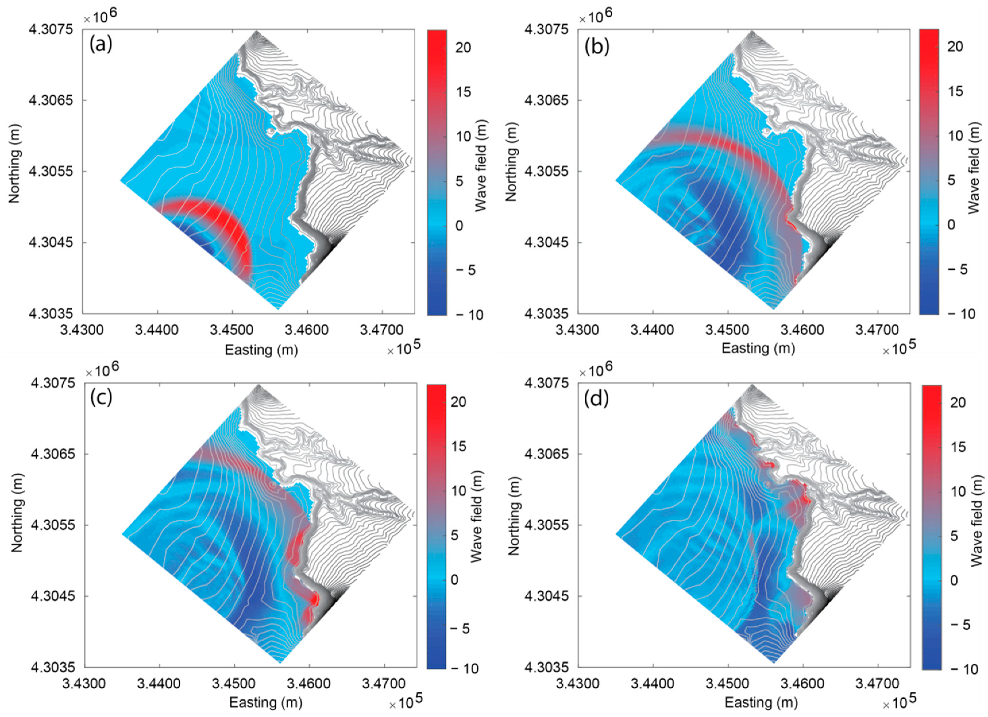
3.2. Wave Propagation and Run-Up

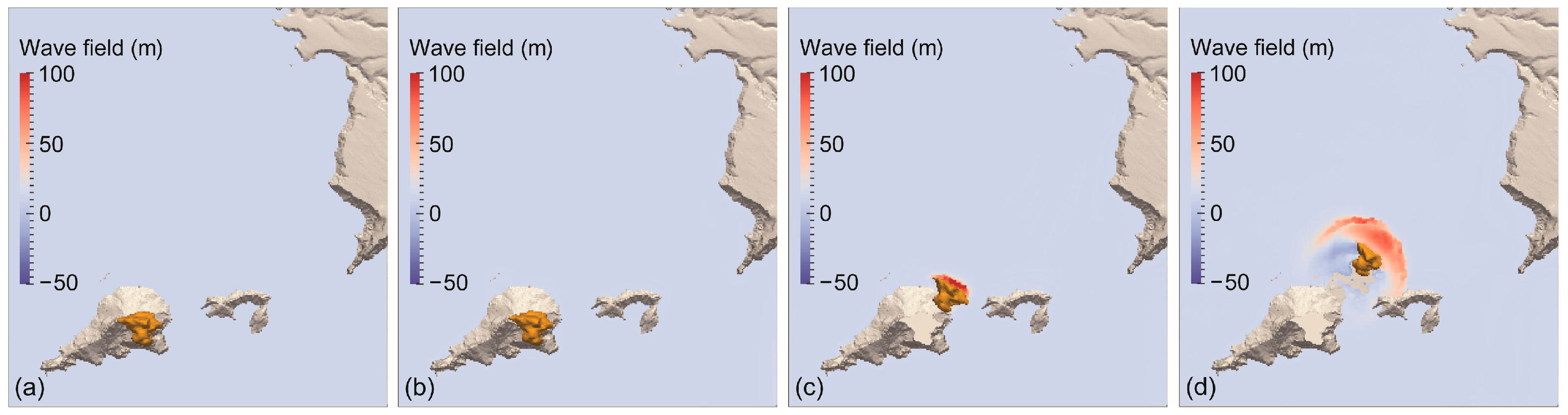
3.2.1. Scenario 1 (Cala d’Hort)

Figure 8a shows the time series of the water surfaces measured every 200 m along the slide axis for 10 locations in total. The primary wave remains the largest wave up to the beach with a maximum wave amplitude of 28.5 m at x = 850 m. This is around 40% less than the input value that was used in SWASH at x = 750 m, which is consistent with the decay found between x = 500 m and x = 750 m in DualSPHysics (Figure 7a). The minimum primary wave amplitude in Figure 8a of 8.7 m is found at x = 2650 m. Figure 8b shows a time series at different distances from Cala d’Hort, with x_b = 0 m corresponding to the still water shoreline (x = 2980 m in the global coordinate system). The maximum wave amplitude of 14.2 m is observed at x_b = − 5 m, with a noticeable increase from x = 2650 m (Figure 8a), which was mainly due to a second wave caused by reflection from the cliffs surrounding the beach (Figure 9) and shoaling effects. The effect of the reflection can be seen at x_b = − 100 m and t = 135 s in Figure 8b.

Figure 9 shows the wave propagation towards Cala d’Hort with four snapshots at different times. This shows that the tsunami front remains circular and the maximum amplitude occurs on the slide axis. Further, Figure 9d shows that the wave reaches the shore 122 s after slide impact. Figure 9c,d clearly confirm the reflections on the southeast cliffs generating the secondary peak in Figure 8b.

The tsunami run-up is investigated next with Figure 10, and five critical points are examined in more detail. The values shown refer to the wet computational grid points with P1 and P4 showing the wet most inland points. Given that the grid resolution is only 30 m, the maximum run-up height is likely to be underestimated by the specified values. P1 is positioned inland of Cala Carbo, which is a smaller beach north of Cala d’Hort where at a terrain elevation of 6 m a maximum inundation depth of 0.23 m is measured. P2 is positioned on the west side of the island Escull de Cala d’Hort where the tsunami generates a run-up height of 5.7 m with a maximum water depth of 4.7 m. The last three points in Figure 10 are all positioned at Cala d’Hort. Point B is on the slide axis near the beach shore where a maximum inundation depth of 14.43 m on a terrain elevation of 0.42 m is measured. The water level starts to decrease towards P3 at the most inland part of the beach with a run-up of 9.24 m and a maximum inundation depth of 11.5 m over the entire event. Finally, the water reaches the maximum terrain elevation of 19.7 m above SWL at P4 and a maximum inundation depth of 1.8 m.

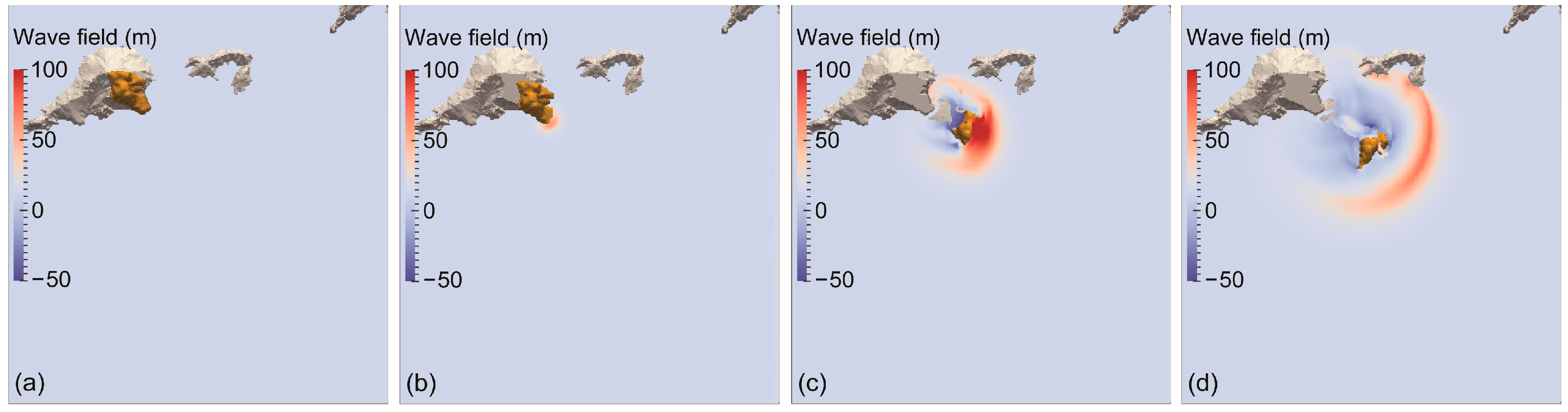
3.2.2. Scenario 2 (Marina de Formentera)

The tsunami propagation and run-up analysis was performed similarly for scenario 2 as for scenario 1. However, the distance between the slide impact and Marina de Formentera is around 10 times larger. Therefore, Figure 11a shows the water surface elevations on the slide axis for every 2000 m only. The maximum amplitude at x = 1500 m is 31 m. The wave decays fast until x = 13,500 m; afterwards, the amplitude stabilises at approximately 2.5 to 3 m whilst approaching the harbour, as the wave decay may be compensated by shoaling effects.

Figure 11b shows how the tsunami approaches the tip of the harbour with a constant wave amplitude of 2.7 m due to the moderate sea bottom slope. Further, Figure 12 shows four snapshots of the tsunami propagation towards Formentera, where the primary tsunami impacts the harbour and coast of the island in Figure 12d after 15 min. It should be noted that the range of the legends in Figure 12b–d have been changed in relation to Figure 12a to reflect the strong reduction in wave amplitude. Figure 12b shows the tsunami diffraction around Cap Llentrisca on Ibiza, which subsequently results in reflection from the cliffs.

The run-up in scenario 2 is investigated in Figure 13, showing how the tsunami floods Marina de Formentera (H), Estany Pudent (P2), and Playa de Illetas (P3), with the maximum horizontal inundation represented by red circles. The elevation at point H is 1.5 m, and the water level reaches 2.7 m above SWL. Further, noticeable run-up affects Cala Saona (P1) on the south, with a terrain elevation of 5.57 m and an inundation depth of 0.57 m. In P2, the tsunami flows into the salt lagoon Estany Pudent, where a water depth of 0.77 m above the terrain elevation can be seen. Then, the tsunami propagates in the lagoon, and dissipates further energy with travel distance as shown in P4, with a tsunami height of only 0.04 m. Finally, parts of Playa de Illetas are flooded, as highlighted with point P3 in Figure 13.

4. Discussion

4.1. Comparison with La Palma Case

Abadie et al. [12] conducted a closely related numerical study by investigating a potential landslide tsunami from La Palma, Canary Islands, and expressed the tsunami decay as a function of the radial distance r from the slide impact location. The tsunami amplitudes a of the present study in both scenarios are compared in Figure 14 with the wave amplitude decays found in Abadie et al. [12]. The amplitudes are shown for the same positions as in Figure 7, Figure 8a and Figure 11a. The solid and dashed lines represent the maximum and minimum decay found by Abadie et al. [12] for slide volumes of 80 km³ and 450 km³, respectively. The tsunami amplitude of scenario 1 decays similarly to $r^{-1.19}$, while the tsunami in scenario 2 decays with $r^{-0.95}$, and lays close to the lower boundary found by Abadie et al. [12]. This small difference is likely due to the different bathymetries in the two cases. Scenario 2 shows a larger water depth and a very mildly sloped seabed, whereas in scenario 1, the shallower water depth and rapidly varying seabed interact more with the tsunami, increasing the decay rate. Mainland Ibiza, which is shown on the north side in Figure 12a, may also have a small effect on the lateral energy spread [29,48], and the wave decay may also change with the wave type (landslide-tsunami propagation in 3D typically involves Stokes-like and cnoidal-like waves [29]). Overall, a consistent wave amplitude decay between the present study and Abadie et al. [12] is found.

4.2. Implications and Limitations

The main purpose of this work is to demonstrate a versatile numerical technique that can be applied to other landslide-tsunami events in reservoirs, lakes, fjords, and the sea. This numerical landslide-tsunami hazard assessment technique for site-specific bathymetric and topographic conditions relies on the two complementing numerical codes DualSPHysics and SWASH; DualSPHysics is well-suited for the violent wave generation process, but is computationally expensive, and may result in unphysical wave decay beyond the coupling location. On the other hand, SWASH deals well with long-distance wave propagation and run-up by taking frequency dispersion and bottom friction into account at small computational cost. It was demonstrated that these two codes combined are capable of resolving the entire landslide-tsunami phenomenon from slide impact, wave generation, and wave propagation to run-up, as well as the inundation of coastal areas.

The landslide-tsunami scenarios investigated herein are hypothetical, and no evidence currently suggests that Es Vedrà may become unstable. Further, the predicted maximum wave amplitudes herein would be extreme values. This is because only subaerial landslides were investigated, which are known to generate larger tsunamis than partially submerged or submarine landslides by given slide volume. Further, extreme slide scenarios resulting in the largest waves were investigated, and it was in addition not possible to fully model the slide basal friction at this stage (the slides are rather modelled as hypermobile [59]). This issue has already been pointed out by Heller et al. [8], who reduced the slide impact velocity by approximately 50% to match the experimental wave amplitudes. In the present work, the calibration and validation tests of DualSPHysics v4.0 with the experimental data presented in Heller et al. [8] was once more performed, resulting in similar conclusions as described by Heller et al. [8], namely that the numerical wave amplitudes are overestimated with an unreduced slide impact velocity. More work is required to fully address this slide kinematics issue. In the meantime, it should be kept in mind that the simulated tsunamis are likely to be larger in the immediate slide impact zone than observed in reality. On the other hand, the wave decay in DualSPHysics was shown to be overpredicted in 3D by Heller et al. [8] (see their Figure 6e,f), such that the too-large slide velocity and wave decay partially compensate each other, and the simulated tsunami amplitudes at the coupling location are expected to be reliable enough for engineering applications. On the other hand, the wave propagation in SWASH is known to work reliably [48].

Finally, even though the wave propagation towards the mainland of Spain was not investigated herein, it is safe to state that a potential landslide tsunami originating from Es Vedrà would be very small at the mainland of Spain due to two main reasons. Firstly, Es Vedrà is less sloped towards the mainland of Spain, such that the slide volume and hence the tsunamis, would be smaller than in the two investigated scenarios. Secondly, the closest point on the mainland of Spain is 85 km away from Es Vedrà, and by applying the decay r^−1.19 that was found towards Cala d’Hort (which is likely to underpredict the decay of the more freely propagating tsunamis towards the mainland of Spain), the resulting wave would only be 0.16 m based on the largest wave amplitude of 133 m in scenario 1. Further, the affected coast of mainland Spain consists mainly of cliffs, which also reduces the damage potential of a hypothetical landslide tsunami from Es Vedrà.

5. Conclusions

This work addressed a numerical technique to conduct landslide-tsunami hazard assessments in reservoirs, lakes, fjords, and the sea. The viability of this technique was demonstrated with hypothetical landslide tsunamis originating from Es Vedrà, offshore Ibiza, under consideration of the site-specific bathymetry and topography. The two numerical codes DualSPHysics and SWASH were applied, thereby combining the strengths in modelling the violent wave generation process of the former with the accurate long-distance wave propagation at the small computational cost of the latter. The coupling of the two codes was carried out by importing the wave profiles and wave kinematics from DualSPHysics into SWASH at a distance where the wave profiles were reasonably stable. Two landslide-tsunami scenarios were investigated by focusing on two particularly exposed locations, namely (i) Cala d’Hort (3 km away from Es Vedrà) and (ii) Marina de Formentera (23 km away from Es Vedrà). The main findings of this study are summarised as follows:

—

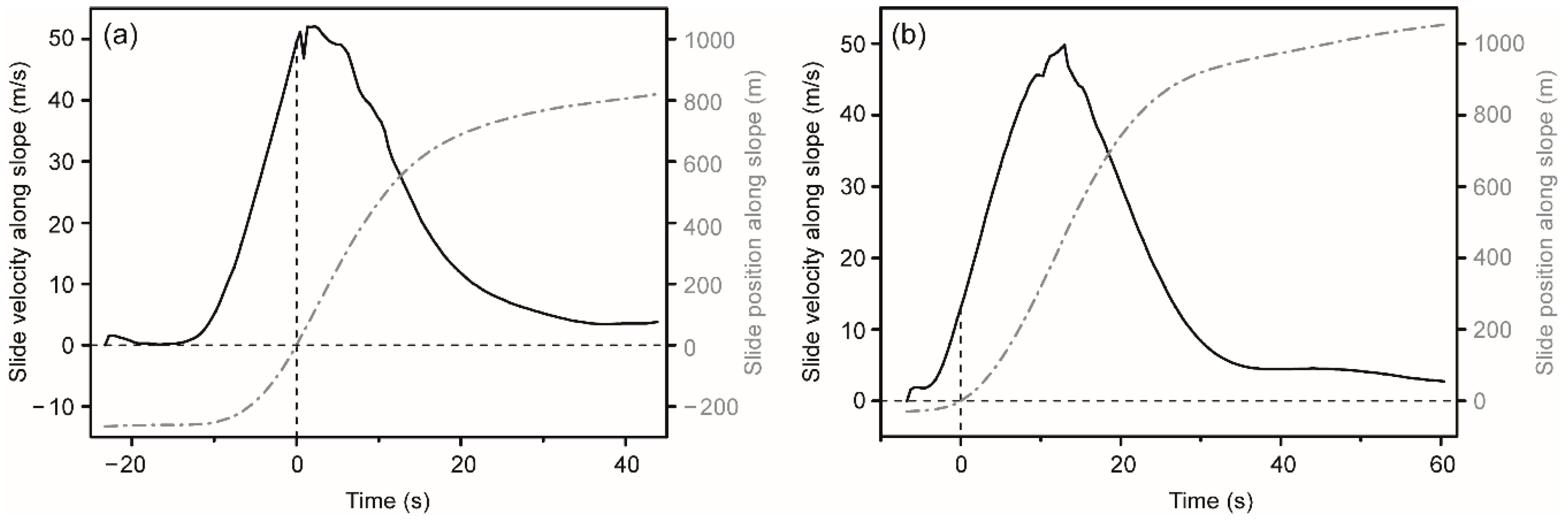
Two different slide–wave interaction phases were observed. (i) At the very beginning, the slide moved faster than the waves, such that the slide propagated below the primary wave crest and additionally elevated the water column and free water surface. (ii) The slide then slowed down such that the waves travelled faster and abruptly decayed due to the increased water depth.

—

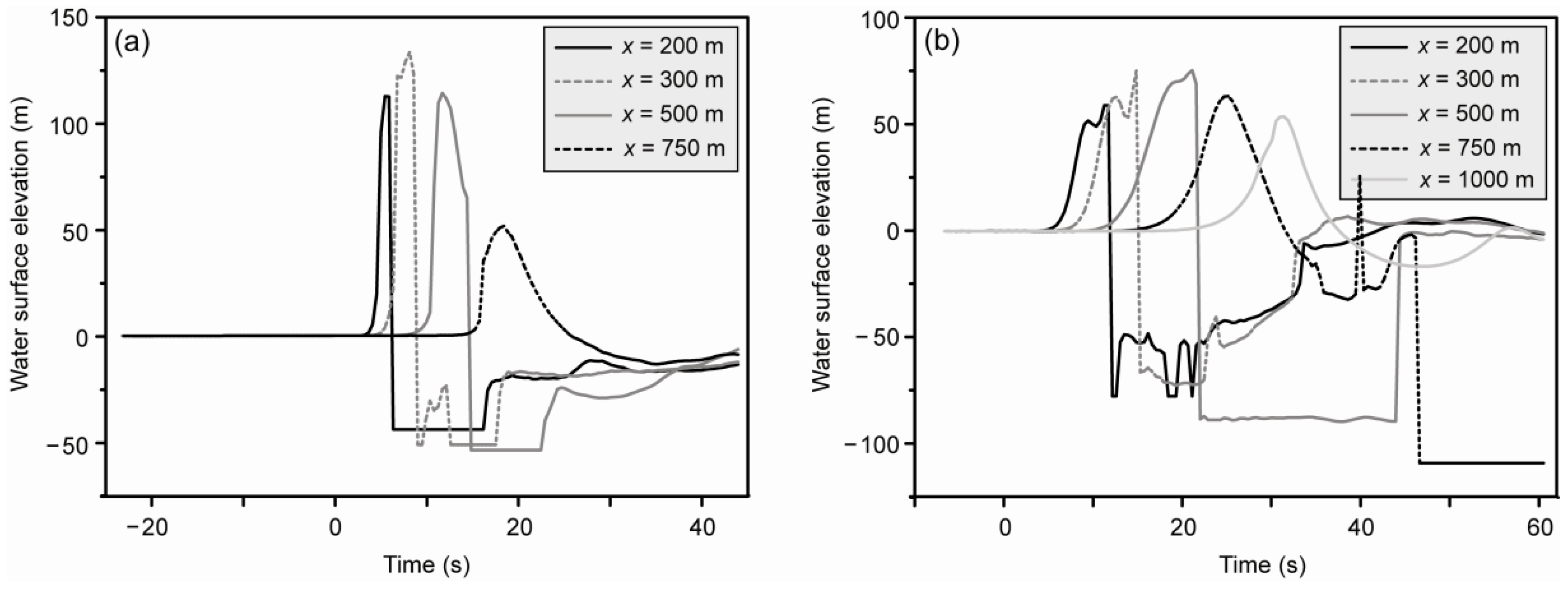
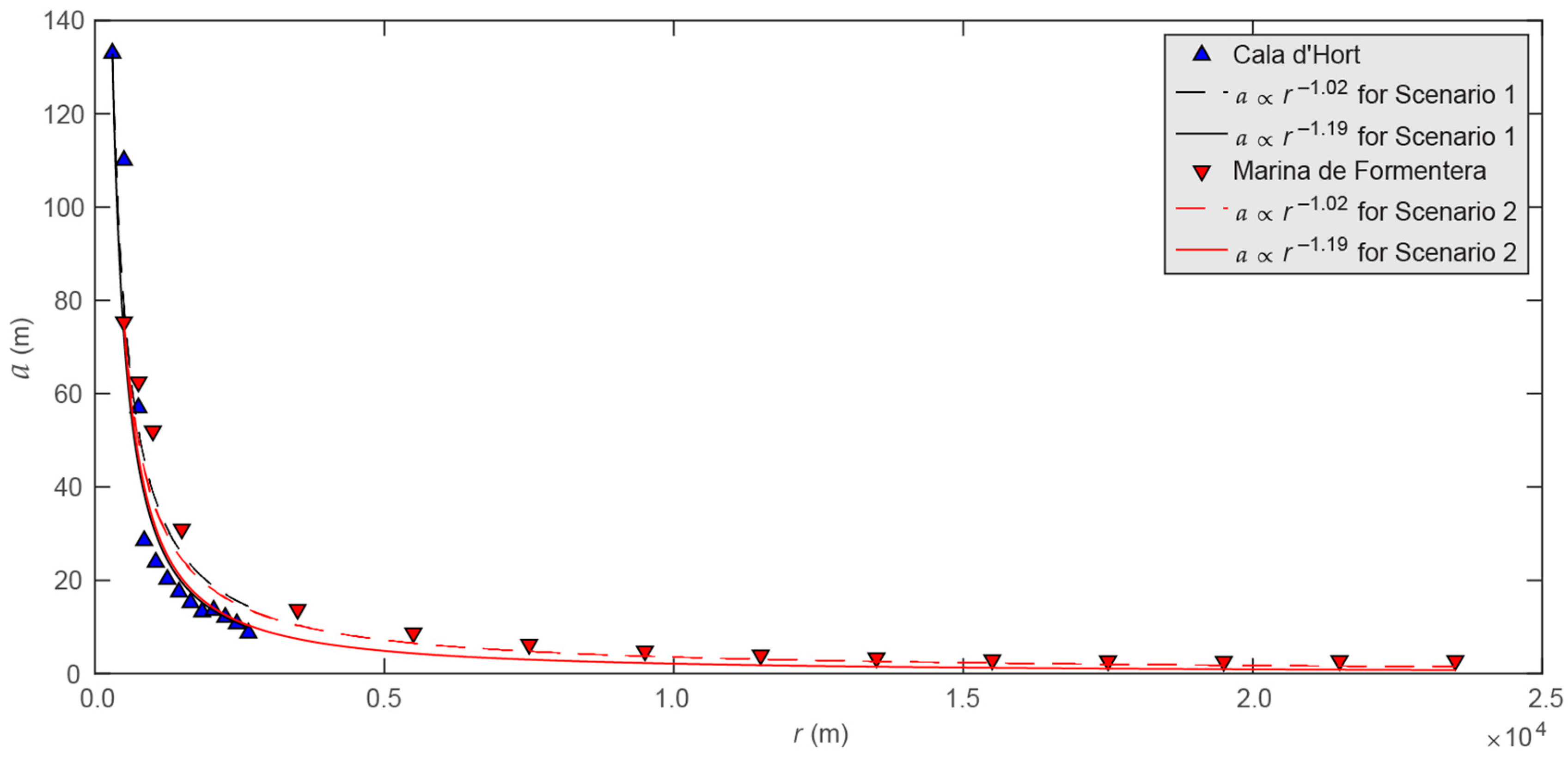
In scenario 1 (Cala d’Hort), the maximum wave amplitude was 133.0 m, reducing to a wave amplitude of 14.2 m at 5 m offshore and a maximum run-up height of over 21.5 m. In scenario 2 (Marina de Formentera), the maximum wave amplitude was 75.4 m, reducing to 2.7 m at 5 m offshore Marina de Formentera, such that the inundation depth was 1.2 m in the populated harbor area. This is significantly smaller than at Cala d’Hort, but may still result in significant devastation due to a larger density of buildings and infrastructure.

—

The proposed numerical technique results likely in an overestimation of the landslide tsunamis because extreme slide scenarios were selected (extreme slide masses, slip orientation, and subaerial slides), and the slide velocity in DualSPHysics is likely to be overpredicted.

—

The proposed numerical technique also provided new insights into 3D landslide-tsunami propagation by considering site-specific bathymetric and topographic conditions.

The change of the landslide-tsunami features by using the laminar viscosity with sub-particle scale turbulence rather than the artificial viscosity for the dissipative terms, the slide kinematics issue and the definition of an exact criterion for the coupling location remain open for future research.

References

1. Panizzo, A.; Girolamo, P.D.; Risio, M.D.; Maistri, A.; Petaccia, A. Great landslide events in Italian artificial reservoirs. Nat. Hazards Earth Syst. Sci. 2005, 5, 733–740. [Google Scholar] [CrossRef] [Green Version]
2. Fuchs, H.; Pfister, M.; Boes, R.; Perzlmaier, S.; Reindl, R. Impulswellen infolge Lawineneinstoss in den Speicher Kühtai. Wasserwirtschaft 2011, 101, 54–60. [Google Scholar] [CrossRef]
3. Fuchs, H.; Boes, R. Berechnung felsrutschinduzierter Impulswellen im Vierwaldstättersee. Wasser Energie Luft 2010, 102, 215–221. [Google Scholar]
4. Gylfadóttir, S.S.; Kim, J.; Helgason, J.K.; Brynjólfsson, S.; Höskuldsson, Á.; Jóhannesson, T.; Harbitz, C.B.; Løvholt, F. The 2014 Lake Askja rockslide-induced tsunami: Optimization of numerical tsunami model using observed data. J. Geophys. Res. Oceans 2017, 122, 4110–4122. [Google Scholar] [CrossRef] [Green Version]
5. Harbitz, C.B.; Glimsdal, S.; Løvholt, F.; Kveldsvik, V.; Pedersen, G.K.; Jensen, A. Rockslide tsunamis in complex fjords: From an unstable rock slope at Åkerneset to tsunami risk in western Norway. Coast. Eng. 2014, 88, 101–122. [Google Scholar] [CrossRef]
6. Watt, S.F.L.; Talling, P.J.; Vardy, M.E.; Heller, V.; Hühnerbach, V.; Urlaub, M.; Sarkar, S.; Masson, D.G.; Henstock, T.J.; Minshull, T.A.; et al. Combinations of volcanic-flank and seafloor-sediment failure offshore Montserrat, and their implications for tsunami generation. Earth Planet. Sci. Lett. 2012, 319, 228–240. [Google Scholar] [CrossRef]
7. Vacondio, R.; Mignosa, P.; Pagani, S. 3D SPH numerical simulation of the wave generated by the Vajont rockslide. Adv. Water Resour. 2013, 59, 146–156. [Google Scholar] [CrossRef]
8. Heller, V.; Bruggemann, M.; Spinneken, J.; Rogers, B.D. Composite modelling of subaerial landslide–tsunamis in different water body geometries and novel insight into slide and wave kinematics. Coast. Eng. 2016, 109, 20–41. [Google Scholar] [CrossRef] [Green Version]
9. Zijlema, M.; Stelling, G. Efficient computation of surf zone waves using the nonlinear shallow water equations with non-hydrostatic pressure. Coast. Eng. 2008, 55, 780–790. [Google Scholar] [CrossRef]
10. Zijlema, M.; Stelling, G.; Smit, P. SWASH: An operational public domain code for simulating wave fields and rapidly varied flows in coastal waters. Coast. Eng. 2011, 58, 992–1012. [Google Scholar] [CrossRef]
11. Sælevik, G.; Jensen, A.; Pedersen, G. Experimental investigation of impact generated tsunami; related to a potential rock slide, Western Norway. Coast. Eng. 2009, 56, 897–906. [Google Scholar] [CrossRef]
12. Abadie, S.M.; Harris, J.C.; Grilli, S.T.; Fabre, R. Numerical modeling of tsunami waves generated by the flank collapse of the Cumbre Vieja Volcano (La Palma, Canary Islands): Tsunami source and near field effects. J. Geophys. Res. Oceans 2012, 117, C05030. [Google Scholar] [CrossRef]
13. Heller, V.; Spinneken, J. Improved landslide-tsunami prediction: Effects of block model parameters and slide model. J. Geophys. Res. Oceans 2013, 118, 1489–1507. [Google Scholar] [CrossRef] [Green Version]
14. Heller, V.; Hager, W.H. Impulse product parameter in landslide generated impulse waves. J. Waterw. Port Coast. Ocean Eng. 2010, 136, 145–155. [Google Scholar] [CrossRef]
15. Heller, V.; Hager, W.H. A universal parameter to predict landslide-tsunamis? J. Mar. Sci. Eng. 2014, 2, 400–412. [Google Scholar] [CrossRef]
16. Evers, F.M.; Hager, W.H. Spatial impulse waves: Wave height decay experiments at laboratory scale. Landslides 2016, 13, 1395–1403. [Google Scholar] [CrossRef]
17. Heller, V.; Hager, W.H.; Minor, H.-E. Landslide Generated Impulse Waves in Reservoirs—Basics and Computation; Swiss Federal Institute of Technology (ETH) Zurich: Zurich, Switzerland, 2009. [Google Scholar]
18. Battaglia, D.; Strozzi, T.; Bezzi, A. Landslide hazard: Risk zonation and impact wave analysis for the Bumbuma Dam-Sierra Leone. Geol. Soc. Territory 2015, 2, 1129–1134. [Google Scholar]
19. BGC Engineering Inc. Appendix 4-E Mitchell Pit Landslide Generated Wave Modelling; BGC Engineering Inc.: Vancouver, BC, Canada, December 2012. [Google Scholar]
20. Gabl, R.; Seibl, J.; Gems, B.; Aufleger, M. 3-D numerical approach to simulate the overtopping volume caused by an impulse wave comparable to avalanche impact in a reservoir. Nat. Hazards Earth Syst. Sci. 2015, 15, 2617–2630. [Google Scholar] [CrossRef] [Green Version]
21. Lüthi, M.P.; Vieli, A. Multi-method observation and analysis of a tsunami caused by glacier calving. Cryosphere 2016, 10, 995–1002. [Google Scholar] [CrossRef] [Green Version]
22. Oppikofer, T.; Hermanns, R.L.; Sandoy, G.; Böhme, M.; Jaboyedoff, M.; Horton, P.; Roberts, N.J.; Fuchs, H. Quantification of casualties from potential rock-slope failures in Norway. Landslides Eng. Slopes. Exp. Theory Pract. 2016, 1537–1544. [Google Scholar]
23. Salazar, F.; Irazábal, J.; Larese, A.; Oñate, E. Numerical modelling of landslide-generated waves with the particle finite element method (PFEM) and a non-Newtonian flow model. Int. J. Numer. Anal. Methods Geomech. 2016, 40, 809–826. [Google Scholar] [CrossRef] [Green Version]
24. Tan, H.; Chen, S. A hybrid DEM-SPH model for deformable landslide and its generated surge waves. Adv. Water Resour. 2017, 108, 256–276. [Google Scholar] [CrossRef]
25. Kesseler, M.; Heller, V.; Turnbull, B. A laboratory-numerical approach for modelling scale effects in dry granular slides. Landslides 2018, 15, 1–15. [Google Scholar] [CrossRef]
26. Fu, L.; Jin, Y.C. Investigation of non-deformable and deformable landslides using meshfree method. Ocean Eng. 2015, 109, 192–206. [Google Scholar] [CrossRef]
27. Shi, C.; An, Y.; Wu, Q.; Liu, Q.; Cao, Z. Numerical simulation of landslide-generated waves using a soil–water coupling smoothed particle hydrodynamics model. Adv. Water Resour. 2016, 92, 130–141. [Google Scholar] [CrossRef] [Green Version]
28. Cremonesi, M.; Frangi, A.; Perego, U. A Lagrangian finite element approach for the simulation of water-waves induced by landslides. Comput. Struct. 2011, 89, 1086–1093. [Google Scholar] [CrossRef]
29. Heller, V.; Spinneken, J. On the effect of the water body geometry on landslide-tsunamis: Physical insight from laboratory tests and 2D to 3D wave parameter transformation. Coast. Eng. 2015, 104, 113–134. [Google Scholar] [CrossRef]
30. Crespo, A.J.C.; Domínguez, J.M.; Rogers, B.D.; Gómez-Gesteira, M.; Longshaw, S.; Canelas, R.; Vacondio, R.; Barreiro, A.; García-Feal, O. DualSPHysics: Open-source parallel CFD solver based on smoothed particle hydrodynamics (SPH). Comput. Phys. Commun. 2015, 187, 204–216. [Google Scholar] [CrossRef]
31. Violeau, D.; Rogers, B.D. Smoothed particle hydrodynamics (SPH) for free-surface flows: Past, present and future. J. Hydraul. Res. 2016, 54, 1–26. [Google Scholar] [CrossRef]
32. Madsen, P.A.; Fuhrman, D.R.; Schäffer, H.A. On the solitary wave paradigm for tsunamis. J. Geophys. Res. 2008, 113, C12012. [Google Scholar] [CrossRef]
33. Narayanaswamy, M.; Crespo, A.J.C.; Gómez-Gesteira, M.; Dalrymple, R.A. SPHysics-FUNWAVE hybrid model for coastal wave propagation. J. Hydraul. Res. 2010, 48, 85–93. [Google Scholar] [CrossRef]
34. Altomare, C.; Domínguez, J.M.; Crespo, A.J.C.; Suzuki, T.; Caceres, I.; Gómez-Gesteira, M. Hybridization of the wave propagation model SWASH and the meshfree particle method SPH for real coastal applications. Coast. Eng. J. 2015, 57, 1550024. [Google Scholar] [CrossRef]
35. Viroulet, S.; Cébron, D.; Kimmoun, O.; Kharif, C. Shallow water waves generated by subaerial solid landslides. Geophys. J. Int. 2013, 193, 747–762. [Google Scholar] [CrossRef] [Green Version]
36. European Marine Observation and Data Network, Bathymetry. Available online: http://portal.emodnet-bathymetry.eu/ (accessed on 15 May 2018).
37. CNIG, Topography. Available online: http://centrodedescargas.cnig.es/CentroDescargas/locale?request_locale=en (accessed on 15 May 2018).
38. Gomez-Gesteira, M.; Rogers, B.D.; Crespo, A.J.C.; Dalrymple, R.A.; Narayanaswamy, M.; Dominguez, J.M. SPHysics—Development of a free-surface fluid solver—Part 1: Theory and formulations. Comput. Geosci. 2012, 48, 289–299. [Google Scholar] [CrossRef]
39. Gomez-Gesteira, M.; Rogers, B.D.; Dalrymple, R.A.; Crespo, A.J.C. State-of-the-art of classical SPH for free-surface flows. J. Hydraul. Res. 2010, 48, 6–27. [Google Scholar] [CrossRef]
40. Tan, H.; Xu, Q.; Chen, S. Subaerial rigid landslide-tsunamis: Insights from a block DEM-SPH model. Eng. Anal. Bound. Elem. 2018, 95, 297–314. [Google Scholar] [CrossRef]
41. Liu, G.R.; Liu, M.B. Smoothed Particle Hydrodynamics: A Meshfree Particle Method, 1st ed.; World Scientific: Singapore, 2003. [Google Scholar]
42. Molteni, D.; Colagrossi, A. A simple procedure to improve the pressure evaluation in hydrodynamic context using the SPH. Comput. Phys. Commun. 2009, 180, 861–872. [Google Scholar] [CrossRef]
43. Monaghan, J.J. Smoothed particle hydrodynamics. Rep. Prog. Phys. 2005, 68, 1703–1759. [Google Scholar] [CrossRef]
44. Monaghan, J.J. Smoothed particle hydrodynamics. Annu. Rev. Astron. Astrophys. 1992, 30, 543–574. [Google Scholar] [CrossRef]
45. Monaghan, J.J. Simulating free surface flows with SPH. J. Comput. Phys. 1994, 110, 399–406. [Google Scholar] [CrossRef]
46. Morris, J.P.; Fox, P.J.; Zhu, Y. Modeling low Reynolds number incompressible flows using SPH. J. Comput. Phys. 1997, 136, 214–226. [Google Scholar] [CrossRef]
47. Crespo, A.J.C.; Gómez-Gesteira, M.; Dalrymple, R.A. Boundary conditions generated by dynamic particles in SPH methods. CMC Comput. Mater. Contin. 2007, 5, 173–184. [Google Scholar]
48. Ruffini, G.; Heller, V.; Briganti, R. Numerical modelling of landslide-tsunami propagation in a wide range of idealised water body geometries. 2018. (in preparation) [Google Scholar]
49. Stelling, G.; Zijlema, M. An accurate and efficient finite-difference algorithm for non-hydrostatic free-surface flow with application to wave propagation. Int. J. Numer. Methods Fluids 2003, 43, 1–23. [Google Scholar] [CrossRef]
50. Zijlema, M.; Stelling, G. Further experiences with computing non-hydrostatic free-surface flows involving water waves. Int. J. Numer. Methods Fluids 2005, 48, 169–197. [Google Scholar] [CrossRef]
51. Blayo, E.; Debreu, L. Revisiting open boundary conditions from the point of view of characteristic variables. Ocean Model. 2005, 9, 231–252. [Google Scholar] [CrossRef] [Green Version]
52. Sommerfeld, A. Die Greensche Funktion der Schwingungsgleichung. Jahresber. Dtsch. Mathematiker-Ver. 1912, 21, 309–353. [Google Scholar]
53. SWASH—User Manual; Version 4.01; Delft University of Technology: Delft, The Netherland, 2016.
54. Nehlich, O.; Fuller, B.T.; Márquez-Grant, N.; Richards, M.P. Investigation of diachronic dietary patterns on the islands of Ibiza and Formentera, Spain: Evidence from sulfur stable isotope ratio analysis. Am. J. Phys. Anthropol. 2012, 149, 115–124. [Google Scholar] [CrossRef] [PubMed]
55. Manger, G.E. Porosity and Bulk Density of Sedimentary Rocks; U.S. G.P.O.: Washington, DC, USA, 1963. [Google Scholar]
56. Hughes, S.A. Physical Models and Laboratory Techniques in Coastal Engineering, 1st ed.; World Scientific: Singapore, 1993. [Google Scholar]
57. Heller, V. Scale effects in physical hydraulic engineering models. J. Hydraul. Res. 2011, 49, 293–306. [Google Scholar] [CrossRef]
58. Wang, J.; Ward, S.N.; Xiao, L. Numerical simulation of the December 4, 2007 landslide-generated tsunami in Chehalis Lake, Canada. Geophys. J. Int. 2015, 201, 372–376. [Google Scholar] [CrossRef] [Green Version]
59. Pudasaini, S.P.; Miller, S.A. The hypermobility of huge landslides and avalanches. Eng. Geol. 2013, 157, 124–132. [Google Scholar] [CrossRef]
60. Huang, B.; Yin, Y.; Chen, X.; Liu, G.; Wang, S.; Jiang, Z. Experimental modeling of tsunamis generated by subaerial landslides: Two case studies of the Three Gorges Reservoir, China. Environ. Earth Sci. 2014, 71, 3813–3825. [Google Scholar]
Figure 1. (a) Plan view of Ibiza and Formentera with Es Vedrà and tsunami propagation towards Cala d’Hort (scenario 1) and Marina de Formentera (scenario 2) marked with red dashed lines (adapted from Google maps); the red dashed square highlights the region shown in (b). (b) Reproduced bathymetry [36] and topography [37] in proximity of Es Vedrà with the range covered by the picture in (c) marked with blue dashed lines. (c) Picture of Es Vedrà taken by V. Heller from Ibiza.
Jmse 06 00111 g001
Figure 2. Central sections of the slide profiles marked in light brown for (a) scenario 1 and (b) scenario 2.
Jmse 06 00111 g002
Figure 3. Convergence test: wave profiles at 2.00 m along the slide axis for different particle spacings dp in scenario 2.
Jmse 06 00111 g003
Figure 4. Time history of the slide velocity and position for (a) scenario 1 and (b) scenario 2; the landslide fronts reach the water surface at position = 0 m and t = 0 s.
Jmse 06 00111 g004
Figure 5. Time history of wave generation in scenario 1 at (a) t = −23.3 s, (b) −9.9 s, (c) 3.5 s, and (d) 16.9 s.
Jmse 06 00111 g005
Figure 6. Time history of wave generation in scenario 2 at (a) t = −6.7 s, (b) 6.7 s, (c) 20.1 s, and (d) 33.5 s.
Jmse 06 00111 g006
Figure 7. Time history of the water surface elevation measured along the slide axes; (a) scenario 1 resulting in a maximum wave amplitude of 133.0 m and (b) scenario 2 resulting in a maximum wave amplitude of 75.4 m.
Jmse 06 00111 g007
Figure 8. Time history of the water surface elevation measured along the slide axis for scenario 1; (a) relative to the slide impact point (x = 0 m) and (b) relative to Cala d’Hort (xb = 0 m and x = 2980 m).
Jmse 06 00111 g008
Figure 9. Time history of wave propagation in scenario 1 at (a) t = 33 s, (b) 66 s, (c) 96 s, and (d) 122 s.
Jmse 06 00111 g009
Figure 10. Maximum run-up heights and water depths at different points of interest in scenario 1.
Jmse 06 00111 g010
Figure 11. Time history of the water surface elevation measured along the slide axis for scenario 2; (a) relative to the slide impact point (x = 0 m) and (b) relative to Marina de Formentera (xh = 0 m and x = 23,665 m).
Jmse 06 00111 g011
Figure 12. Time history of wave propagation in scenario 2 at (a) t = 65 s, (b) 305 s, (c) 605 s, and (d) 905 s.
Jmse 06 00111 g012
Figure 13. Maximum run-up heights and water depths at different points of interest in scenario 2.
Jmse 06 00111 g013
Figure 14. Comparison of wave amplitude a decay over radial distance r for both scenarios with maximum and minimum decay found by Abadie et al. [12].
Jmse 06 00111 g014