Hemp Cables, a Sustainable Alternative to Harmonic Steel for Cable Nets

Abstract

Recent developments in the field of materials engineering have allowed for the use of natural materials for common structural elements, instead of traditional materials, such as steel or concrete. In this context, hemp is a very interesting material for structural building design. This paper proposes the use of hemp cables for roofs with hyperbolic paraboloid cable nets, which sees the use of a sustainable material for structure, thus having a very low environmental impact, in terms of structural thickness and amount of material. The paper discusses five different plan sizes and two different hyperbolic paraboloid surface radius of curvatures. The cable traction, which gives the cable net stiffness, was varied in order to give a parametric database of structural response. Three dimensional geometrically nonlinear analyses were carried out on different geometries (i.e., 10), cable net stiffnesses (i.e., 8), and materials (i.e., 2). Traditional harmonic steel and hemp cables are compared, in terms of vertical displacements and natural periods under dead and permanent loads.

1. Introduction

Hemp is the same plant as marijuana, and its scientific name is Cannabis sativa. For thousands of years, hemp was used to make dozens of commercial products, like paper, rope, canvas, and textiles.

Hemp has recently been rediscovered as a plant that has enormous environmental, economic, and commercial potential. The potential of hemp for paper production is enormous. According to the U.S. Department of Agriculture, one acre of hemp can produce 4 times more paper than one acre of trees. All types of paper products can be produced from hemp. Hemp can also be substituted for cotton to make textiles. Hemp fiber is 10 times stronger than cotton, and can be used to make all types of clothing. Cotton grows only in warm climates, and requires enormous amounts of water, which is contrary to hemp growth conditions.

In the past, the majority of cities and towns in the world had an industry making hemp rope and, in fact, Russia was the world’s largest producer and best-quality manufacturer, supplying 80% of the Western world’s hemp, from 1740 until 1940. Until 1937, 70–90% of all rope, twine, and cordage was made from hemp [1].

Since the late twentieth century, along with the sharpening increase of global environmental pollution, people’s eyes have turned to non-polluting, antibacterial resources which can be recycled for use, and cannabis has re-entered into people’s vision [2]. Thanks to the continuous developments in textile technology, the fineness of hemp fibers continues to improve.

Key researchers analyzed, through the study of the status of hemp fiber, high temperature resistance, heat resistance, and other properties [3,4,5,6]. For example, they explored hemp fiber insulation regarding anti-radiation and anti-mildew and antibacterial performance, and through the analysis of hemp fiber temperature, thermal conductivity, permeability, and other properties were investigated [7,8].

Building materials that substitute wood can be made from hemp. These wood-like building materials are stronger than wood, and can be manufactured cheaper. Using these hemp-derived building materials would reduce building costs and save even more trees [9]. In addition, different applications of hemp in the field of building construction have recently been developed as, for example, Hemplime (HL), a sustainable low-carbon composite building material that combines hemp shiv with formulated lime-based binders [10].

However, codes of practice neglect hemp as a structural material, and there is a lack of information for designers to follow, thus reducing the hemp potential.

In particular, hemp is mostly used for ropes because it has a great resistance to traction (i.e., about 300 MPa). In addition, as is the case for most sailing ropes, ropes and cables for structural uses require high stiffness values to maximize their effectiveness and enable precise control displacement [11]. Based on these reasons, hemp, theoretically, can be used for all kinds of tensile structures as, for example, suspended bridges or cable nets, usually built from cables made of harmonic steel.

This paper does not discuss the durability of materials, hemp, and harmonic steel. The reason is that the durability of cable material depends on protective layers that can be the same for both materials.

In fact, the use of hemp, which is usually cheaper than harmonic steel, may improve cable net diffusion in favor of a cost–benefit balance for structures, and is particularly convenient for covering large spans for both temporary or permanent conditions. It is commonly used for sport arenas, but recent studies have shown that they can also be used for music halls [12,13]. The strength of cable net roofs is their lightness and their minimum thickness compared to the span. The lightness of these roofs improved using hemp cables because the hemp weight (i.e., about 1500 kg/m³) is about one-fifth that of steel per cubic meter.

However, the structural lightness renders them prone to wind action and, in particular, the structural reliability may be affected by local and global instability, due to the wind–structure interaction, similar to that of suspended bridges [3,14,15,16] contrarily for concrete bridge that are more sensitive to seismic action [17]. This is a crucial topic for tensile structure design and, in the case of the cable net, it is general due to the loss of the initial strain by cables. Codes of Practice (such as Ref. [18,19,20,21,22,23,24], IS 875 Part 3 commented in Ref. [25,26,27]) neglect hyperbolic paraboloid cable net–wind interaction.

Many studies have discussed this problem and have confirmed that the cable nets and membrane need to be designed by taking into account the dynamic instability given by wind–structure interaction, but they have only given information about specific cases of study. Some examples are shown in Ref. [28,29,30,31,32,33,34,35,36,37,38,39,40,41,42,43]. Similarly, a great number of wind tunnel test campaigns have been described in the literature, but have focused on particular cases of study. Key examples are shown in Ref. [44,45,46,47,48,49,50,51].

For this reason, data are not standardized for different geometries. Some examples follow a parametric approach, given that aerodynamic data are useful for designers (for example, Ref. [52,53,54]). These studies aid designers in estimating the wind action on roofs before carrying out expensive wind tunnel tests. Other publications have given simplified pressure coefficient maps that synthetize parametric results for a great number of different geometries as, for example, [52,55]. Generalizable information about the wind action on these kinds of roofs is presented in Ref. [25,37,56]. Finally, the lightness of the roof makes tensile structures sensitive to local extreme values of the wind action that can cause cable connections to collapse. Rizzo et al. [57] recently investigated this aspect, and Liu et al. [58] indicated the peaks factor distributions on a hyperbolic paraboloid roof.

This paper is focused on the statically and dynamically balanced structural design under dead and permanent loads, which is a preparatory crucial phase to investigate the wind–structure interaction. Section 3 covers some notions concerning cable net base theory.

In order to achieve this goal, two different surfaces of hyperbolic paraboloid (i.e., two different radius of curvature), five different square plan sizes (i.e., 100, 80, 60, 40, and 20 m) and two different materials (i.e., hemp and harmonic steel) are considered in this study. It is important to note that the study is focused on structures with medium and small spans, in order to promote the dissemination about these kinds of structures. The purpose is to use cable nets as an alternative to steel truss or wood structures for small and medium sport arenas. That is because they have an efficient cost–benefit ratio also for small spans [31]. In addition, it is important to specify that the geometrical span range (i.e., from 100 to 20) was chosen as a linear variation of the span, in order to give a measure of the structural response variation as function of the span.

For the purpose of comparing only the cable net performances, the distance between load-bearing and stabilizing cables are taken as constant for all geometries and span lengths. For this reason, the curvature of the roof with the smaller spans (i.e., 40 m or 20 m) is badly reproduced. However, the distance between cables can be proportionally varied as a function of the span. All geometries are designed for eight different values of cable traction (i.e., 100, 200, 400, 600, 1000, 2000, 4000, and 8000 kN for load-bearing cables), in order to investigate the dynamic dependence on cable net stiffness. Finally, parametric curves of vertical displacements and the first natural period are given for a preliminary design of structures.

The first natural frequency (i.e., mode with biggest participating mass) was estimated, taking into account masses given by structural and permanent loads, and it was given considering the initial pretension of cables. It is known that the cables strain and stress vary significantly under snow or wind action. This study is only focused on the structural response under structural weight and permanent loads. For this reason, equations and figures, that illustrate structural response variation, only refer to the structural weight and permanent loads.

In this research, only the cable net is investigated. For this reason, the border structures are restrained. In addition, the membrane contribution, in terms of roof stiffness, is not considered, in order to only study the cable net performances.

2. The Geometrical Sample

The cable net is made of two orders of cables, upward and downward. The geometry is given by Equation (1). In this study, parameter c is equal to 1.

In Equation (1), x, y, and z are the spatial variables; x₀, y₀, and z₀ are the coordinates of the origin of the axes; and a, b, and c are the geometric coefficients of the function [31,59].

$$\frac{{\left(X-x_0\right)}^2}{a^2}-\frac{{\left(Y-y_0\right)}^2}{b^2}=\frac{\left(Z-Z_0\right)}{c}; 1/c=1$$

(1)

Under gravitational loads (i.e., dead, permanent loads, or snow action), the upward cables are load-bearing, whereas the downward cables are stabilizing cables. Under suction (i.e., upward action as, for example, wind action) the order is inverse. Strong winds can affect the structural reliability because upward cables are drawn upwards enough to lose their strains and, consequently, their initial geometries. The same can happen for downward cables under extreme snow action.

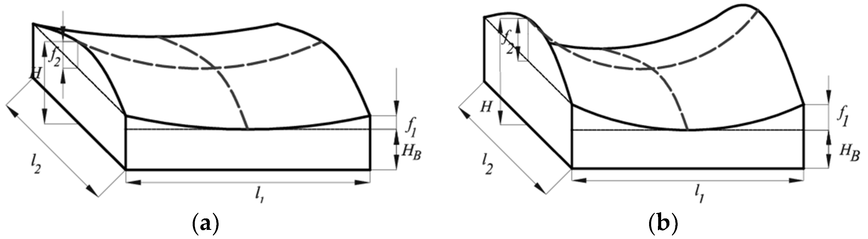
Figure 1 shows the geometrical parameters listed in

Table 1. Geometrical sample.

Geometry	Model	l1 (m)	l2 (m)	f1 (m)	f2 (m)	H (m)
(1)	1	100.00	100.00	3.33	6.67	10.00
	2	80.00	80.00	2.66	5.34	8.00
	3	60.00	60.00	2.00	4.00	6.00
	4	40.00	40.00	1.33	2.67	4.00
	5	20.00	20.00	0.66	1.37	2.00
(2)	1	100.00	100.00	5.55	11.11	16.66
	2	80.00	80.00	4.44	8.89	13.33
	3	60.00	60.00	3.33	6.66	10.00
	4	40.00	40.00	2.22	4.44	6.66
	5	20.00	20.00	1.11	2.22	3.33

for the investigated geometries (1) and (2). The parameters l₁, f₁, l₂, and f₂ are the upward and downward cable sags and spans, respectively. For the square plan, l₁ is equal to l₂. H is the sum of f₁ + f₂ and, in this research, it was assumed to equal to 1/10 (i.e., geometry (1)) and 1/6 (i.e., geometry (2)) of l₁ [60]. The geometry was chosen based on the geometrical parametrization, as a function of the optimal structural performances of the net, given by [60].

3. Geometrically Nonlinear Analyses

3.1. Cable Net Calculation

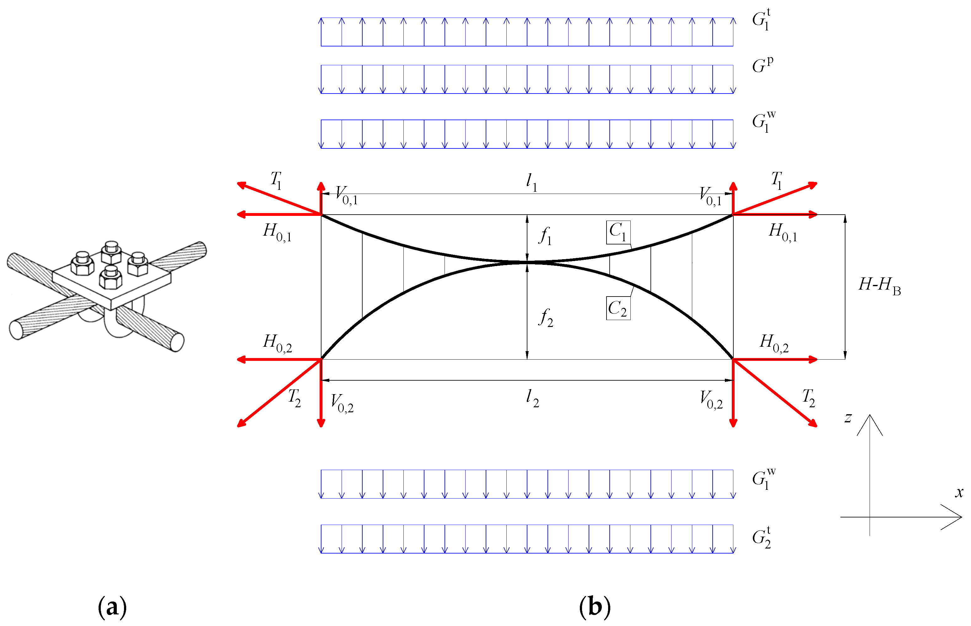
As was discussed previously, hyperbolic paraboloid cable nets have two orders of cables (i.e., C₁ and C₂ in Figure 2) that usually have the same span, but different sags. Consequently, upward and downward cables have different traction, given by different section areas or different strain values. The cable net nodes are connected for vertical displacements according to Figure 2a, that shows an example of node connection.

Cable traction gives two force components to anchoring structures: vertical and horizontal. Horizontal forces become greater as the cable sag becomes smaller. For this reason, greater cable sags generally give smaller anchorage structures, that are less expensive supporting structures. The simplified scheme of the cable net is illustrated in Figure 3b. The two-dimensional model, named the rope-beam, requires balance, given by H_0,1 = H_0,2 for each load action.

The applied load, after construction and without snow and wind (Figure 3a), corresponds to the sum of the cable weight (i.e., in the following dead loads, G_1,2^w), permanent loads (i.e., 0.5 kN/m², G^p), and initial pretension (G_1,2^t). Referring to Figure 2b, the load balance is given by G = +G^p (downward) + G₁^w (downward) + G₁^t (upward) + G₂^w (downward) + G₂^t (downward) = 0.

Referring to Figure 2b, the initial cable tractions, $T_{0,1}$ and $T_{0,2}$, are evaluated as reported in Equations (2) and (3); their horizontal components, $H_{0,1}$ and $H_{0,2}$, are given by Equations (3) and (4). G is the P_0,1 load, and it varies between dead, permanent, snow, or wind action.

The dead and permanent loads are considered load condition “zero”. For this reason, traction and strain have the subscript “0”.

$$T_{0,1}=H_{0,1}\sqrt{1+16{\left(\frac{f_1}{L_1}\right)}^2}$$

(2)

$$T_{0,2}=H_{0,2}\sqrt{1+16{\left(\frac{f_2}{L_2}\right)}^2}$$

(3)

$$H_{0,1}=\frac{\mathrm{G}{L}_1{}^2}{8f_1}=\frac{T_{0,1}}{1+16{\left(\frac{f_1}{L_1}\right)}^2}$$

(4)

$$H_{0,2}=\frac{\mathrm{G}{L}_2{}^2}{8f_2}=\frac{T_{0,2}}{1+16{\left(\frac{f_2}{L_2}\right)}^2}$$

(5)

An initial traction value (i.e., $T_{0,1}$ and $T_{0,2}$) is fixed, in order to have $H_{0,1}=H_{0,2}$, and the geometry is consequently defined. The goal is to obtain the minimum vertical displacement in order to maintain the theoretical geometrical configuration. Cable traction and, in particular, the horizontal components of cable traction (i.e., $H_{0,1};H_{0,2}$), closely affect the anchorage structure sizes and cable stiffness.

For greater tractions, there are smaller displacements but bigger anchorage sizes, too. In addition, cable traction affects the cable section areas because the material limit of stress has to be respected. In summary, the fixed cable material and the chosen exercise stress ($\sigma$) impose the cable strain ($\epsilon$) according to Equation (6), which is Hooke’s law. When the cable tractions (i.e., $T_{0,1}$ and $T_{0,2}$) are fixed, the cable areas are defined, too, according to Equation (7), which is a part of the Navier equation.

$$\sigma =E·\epsilon$$

(6)

$$A=T_{0,i}/\mathsf{\sigma }$$

(7)

In this paper, in order to evaluate the geometry dependence on cable traction for both harmonic steel and hemp, eight different values of cable tractions (i.e., from (A) to (H)) are considered.

Cable values are summarized in

Table 2. Mechanical parameters after fixing the initial strength 0.0035 for steel and 0.0047 for hemp.

Material	Geometry	Model (Span Sizes)	Analysis	${\mathit{T}}_{0,1}\left(\mathbf{kN}\right)$	${\mathit{T}}_{0,2}\left(\mathbf{kN}\right)$	${\mathit{A}}_1\left({\mathbf{m}}^2\right)$	${\mathit{A}}_2\left({\mathbf{m}}^2\right)$
Harmonic Steel	(1)	From 1 to 5	(A)	100.0	105.2	0.00017	0.00018
			(B)	200.0	210.5	0.00035	0.00037
			(C)	400.0	421.0	0.00070	0.00073
			(D)	600.0	631.4	0.00100	0.00110
			(E)	1000.0	1052.4	0.00170	0.00180
			(F)	2000.0	2104.8	0.00350	0.00370
			(G)	4000.0	4209.6	0.00700	0.00730
			(H)	8000.0	8419.2	0.01390	0.01460
	(2)	From 1 to 5	(A)	100.0	114.1	0.00017	0.00018
			(B)	200.0	228.2	0.00035	0.00037
			(C)	400.0	456.5	0.00070	0.00073
			(D)	600.0	684.7	0.00100	0.00110
			(E)	1000.0	1141.2	0.00170	0.00180
			(F)	2000.0	2282.4	0.00350	0.00370
			(G)	4000.0	4564.7	0.00700	0.00730
			(H)	8000.0	9129.4	0.01390	0.01460
Hemp	(1)	From 1 to 5	(A)	100.0	105.2	0.00067	0.00070
			(B)	200.0	210.5	0.00130	0.00140
			(C)	400.0	421.0	0.00270	0.00280
			(D)	600.0	631.4	0.00400	0.00420
			(E)	1000.0	1052.4	0.00670	0.00700
			(F)	2000.0	2104.8	0.01330	0.01400
			(G)	4000.0	4209.6	0.02670	0.02810
			(H)	8000.0	8419.2	0.05330	0.05610
	(2)	From 1 to 5	(A)	100.0	114.1	0.00067	0.00070
			(B)	200.0	228.2	0.00130	0.00140
			(C)	400.0	456.5	0.00270	0.00280
			(D)	600.0	684.7	0.00400	0.00420
			(E)	1000.0	1141.2	0.00670	0.00700
			(F)	2000.0	2282.4	0.01330	0.01400
			(G)	4000.0	4564.7	0.02670	0.02810
			(H)	8000.0	9129.4	0.05330	0.05610

.

Considering only dead and permanent loads, the initial stress of materials was fixed at 50% of the ultimate stress, estimated at 1200 MPa for harmonic steel and 300 MPa for hemp [61]. This is because the snow action increases the stress on load-bearing cables (i.e., upward cables), whereas the wind suction increases the stress on the stabilizing cables (i.e., downward cables).

In addition, for analyses, the material weight was estimated at 78.5 kN/m³ for steel and 14.90 kN/m³ for hemp, while the Young’s modulus was estimated at 165,000 MPa for steel and 32,000 MPa for hemp [61,62,63,64].

All values of section areas, and traction of the two orders of cables, are summarized in Table 2 for both materials (i.e., steel and hemp), for both geometries (i.e., (1) and (2)), and all span sizes (i.e., 100, 80, 60, 40, and 20 m) are illustrated in Figure 1.

3.2. Results

Static and modal analyses are carried out by TENSO (2011), a non-commercial software that includes modules for simulating cable and beam finite element models, and for the study of wind–structure interaction phenomena with the generation of wind speed time histories and simulation of various aeroelastic loads. The main cables are discretized as rectilinear cable segments [15,16,59].

The global stiffness matrix is updated at each load step by assembling the stiffness submatrices of the elements, and updated so as to account for the strain found at the previous time step. In this way, the software considers the geometric nonlinearity of the structure.

The TENSO software first solves for the static equilibrium of the structure under dead, gravity, and construction loads (prior to the application of the wind loads) through nonlinear static analysis, two methods are simultaneously used: a step-by-step incremental method and a “subsequent interaction” method with variable stiffness matrix (secant method). The secant method is a finite-difference approximation of Newton–Raphson’s modified method for systems of nonlinear algebraic equations.

All geometries listed in Table 1 are modelled with a FEM model. They were calculated in order to estimate the maximum (i.e., located at the center of the roof) vertical displacements, and the first ten natural frequencies and periods.

For the sake of brevity, only the value of the first natural frequency and period is discussed in this paper, even though the values of other frequencies followed the same trend of the first.

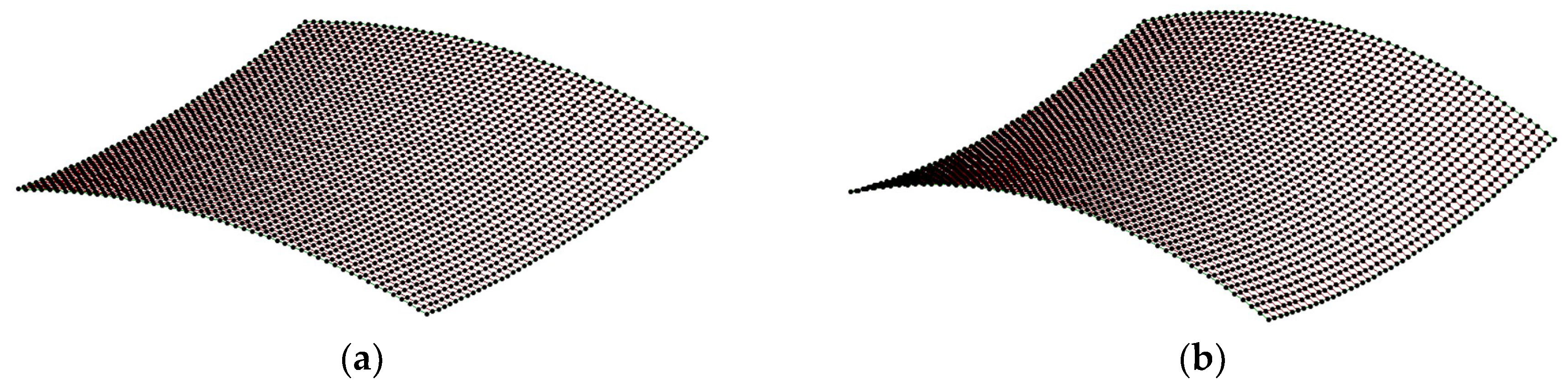
Figure 3 shows as an example the FEM model for both geometries (i.e., (1) and (2), illustrated in Figure 1), and span size equal to 100 m (Figure 3a,b). Figure 3c shows the typical first mode shape for all span sizes (i.e., from 100 to 20 m) that are the same for geometry (1) and (2).

It is obvious that the cable areas and the plan sizes (i.e., l₁ and l₂) closely affect the weight of the cable net and, consequently, the masses of the structure, listed in

Table 3. Geometry (1) modal analyses results.

Geometry	Model	Analysis	Masses		Mode 1st
			Harmonic Steel	Hemp	Harmonic Steel		Hemp
			${\mathit{M}}_{\mathit{i}}$ $(\frac{\mathbf{k}\mathbf{g}}{{\mathbf{m}}^2})$	${\mathit{M}}_{\mathit{i}}$ $(\frac{\mathbf{k}\mathbf{g}}{{\mathbf{m}}^2})$	$\mathit{\phi }$ (Hz) Mode 1st	$\mathit{t}$ (s) from 1st to 10th Modes	$\mathit{\phi }$ (Hz) Mode 1st	$\mathit{t}$ (s) from 1st to 10th Modes
(1)	1	(A)	5.23	5.20	0.0402	24.90	0.0380	26.33
		(B)	5.37	5.30	0.0462	21.66	0.0445	22.48
		(C)	5.64	5.49	0.0659	15.18	0.0657	15.21
		(D)	5.92	5.69	0.0794	12.59	0.0807	12.39
		(E)	6.46	6.09	0.1012	9.88	0.1031	9.70
		(F)	7.83	7.09	0.1342	7.45	0.1368	7.31
		(G)	10.57	9.08	0.1645	6.08	0.1727	5.79
		(H)	16.04	13.06	0.1890	5.29	0.2041	4.90
	2	(A)	5.23	5.20	0.0467	21.42	0.0443	22.59
		(B)	5.37	5.29	0.0572	17.48	0.0558	17.92
		(C)	5.64	5.49	0.0839	11.92	0.0835	11.97
		(D)	5.91	5.69	0.1007	9.93	0.1021	9.79
		(E)	6.46	6.09	0.1277	7.83	0.1299	7.70
		(F)	7.82	7.08	0.1686	5.93	0.1718	5.82
		(G)	10.54	9.06	0.2066	4.84	0.2165	4.62
		(H)	15.98	13.02	0.2370	4.22	0.2558	3.91
	3	(A)	5.23	5.20	0.0573	17.44	0.0551	18.14
		(B)	5.37	5.29	0.0784	12.75	0.0774	12.92
		(C)	5.64	5.49	0.1138	8.79	0.1126	8.88
		(D)	5.91	5.69	0.1385	7.22	0.1376	7.27
		(E)	6.45	6.08	0.1733	5.77	0.1739	5.75
		(F)	7.80	7.06	0.2252	4.44	0.2304	4.34
		(G)	10.49	9.02	0.2755	3.63	0.2899	3.45
		(H)	15.89	12.95	0.3175	3.15	0.3425	2.92
	4	(A)	5.23	5.19	0.0819	12.21	0.0807	12.39
		(B)	5.36	5.29	0.1218	8.21	0.1258	7.95
		(C)	5.63	5.48	0.1739	5.75	0.1715	5.83
		(D)	5.89	5.68	0.2105	4.75	0.2088	4.79
		(E)	6.42	6.06	0.2625	3.81	0.2632	3.80
		(F)	7.75	7.03	0.3401	2.94	0.3472	2.88
		(G)	10.40	8.96	0.4167	2.40	0.4348	2.30
		(H)	15.70	12.82	0.4785	2.09	0.5155	1.94
	5	(A)	5.22	5.19	0.1742	5.74	0.1704	5.87
		(B)	5.35	5.28	0.2513	3.98	0.2463	4.06
		(C)	5.60	5.46	0.3521	2.84	0.3472	2.88
		(D)	5.85	5.65	0.4255	2.35	0.4202	2.38
		(E)	6.35	6.01	0.5291	1.89	0.5291	1.89
		(F)	7.61	6.92	0.6849	1.46	0.6993	1.43
		(G)	10.12	8.75	0.8403	1.19	0.8772	1.14
		(H)	15.15	12.41	0.9709	1.03	1.0417	0.96

and

Table 4. Geometry (2) modal analyses results.

Geometry	Model	Analysis	Masses		Mode 1st
			Harmonic Steel	Hemp	Harmonic Steel		Hemp
			${\mathit{M}}_{\mathit{i}}$ $(\frac{\mathbf{k}\mathbf{g}}{{\mathbf{m}}^2})$	${\mathit{M}}_{\mathit{i}}$ $(\frac{\mathbf{k}\mathbf{g}}{{\mathbf{m}}^2})$	$\mathit{\phi }$ (Hz) Mode 1st	$\mathit{t}$ (s) from 1st to 10th modes	$\mathit{\phi }$ (Hz) Mode 1st	$\mathit{t}$ (s) from 1st to 10th Modes
(2)	1	(A)	5.23	5.20	0.0432	23.17	0.0401	24.91
		(B)	5.37	5.30	0.0570	17.54	0.0532	18.81
		(C)	5.65	5.50	0.0825	12.12	0.0793	12.61
		(D)	5.92	5.70	0.0981	10.19	0.0964	10.37
		(E)	6.47	6.10	0.1239	8.07	0.1222	8.18
		(F)	7.85	7.10	0.1629	6.14	0.1610	6.21
		(G)	10.60	9.10	0.1988	5.03	0.2024	4.94
		(H)	16.10	13.10	0.2278	4.39	0.2392	4.18
	2	(A)	5.23	5.20	0.0508	19.70	0.0476	21.00
		(B)	5.37	5.30	0.0730	13.70	0.0679	14.72
		(C)	5.64	5.50	0.1043	9.59	0.1002	9.98
		(D)	5.92	5.69	0.1236	8.09	0.1215	8.23
		(E)	6.46	6.09	0.1558	6.42	0.1536	6.51
		(F)	7.83	7.09	0.2041	4.90	0.2020	4.95
		(G)	10.57	9.08	0.2494	4.01	0.2538	3.94
		(H)	16.04	13.06	0.2857	3.50	0.2950	3.39
	3	(A)	5.23	5.20	0.0668	14.98	0.0628	15.92
		(B)	5.37	5.29	0.0988	10.12	0.0938	10.66
		(C)	5.64	5.49	0.1403	7.13	0.1342	7.45
		(D)	5.91	5.69	0.1692	5.91	0.1631	6.13
		(E)	6.45	6.08	0.2105	4.75	0.2049	4.88
		(F)	7.81	7.07	0.2725	3.67	0.2703	3.70
		(G)	10.52	9.04	0.3322	3.01	0.3390	2.95
		(H)	15.95	12.99	0.3831	2.61	0.4016	2.49
	4	(A)	5.23	5.19	0.1043	9.59	0.0984	10.16
		(B)	5.36	5.29	0.1511	6.62	0.1437	6.96
		(C)	5.63	5.48	0.2123	4.71	0.2033	4.92
		(D)	5.90	5.68	0.2558	3.91	0.2463	4.06
		(E)	6.43	6.07	0.3175	3.15	0.3086	3.24
		(F)	7.76	7.04	0.4098	2.44	0.4082	2.45
		(G)	10.43	8.98	0.5025	1.99	0.5102	1.96
		(H)	15.76	12.86	0.5780	1.73	0.6061	1.65
	5	(A)	5.22	5.19	0.2160	4.63	0.2041	4.90
		(B)	5.35	5.28	0.3067	3.26	0.2915	3.43
		(C)	5.60	5.46	0.4274	2.34	0.4098	2.44
		(D)	5.85	5.65	0.5128	1.95	0.4950	2.02
		(E)	6.36	6.02	0.6369	1.57	0.6211	1.61
		(F)	7.62	6.93	0.8264	1.21	0.8197	1.22
		(G)	10.15	8.77	1.0204	0.98	1.0309	0.97
		(H)	15.20	12.45	1.1765	0.85	1.2195	0.82

.

Table 3 and Table 4 give a list of the first natural frequency and period of geometry (1) (i.e., Table 3) and (2) (i.e., Table 4), for the five span sizes considered (i.e., l₁ = l₂ = 100; 80; 60; 40 and 20 m) and for the eight cable tractions. The tables also give the mass (M_i) per square meter for a generic node i in the middle of the roof.

4. Results

The mass values listed in Table 3 and Table 4 show substantial similar values between harmonic steel and hemp cable nets for cable traction less than 2000 kN, for both geometry (1) and (2).

Table 5. Measure ($\mathit{\delta }\mathit{\gamma }\%$) of the masses difference between harmonic steel and hemp cable net.

Geometry	T1 (kN)	l1 (m)
		100	80	60	40	20
(1)	100	0.6	0.6	0.6	0.8	0.6
	200	1.3	1.5	1.5	1.3	1.3
	400	2.7	2.7	2.7	2.7	2.6
	600	4.0	3.9	3.9	3.7	3.5
	1000	6.1	6.1	6.1	5.9	5.7
	2000	10.4	10.5	10.5	10.2	10.0
	4000	16.4	16.3	16.3	16.1	15.7
	8000	22.8	22.7	22.7	22.5	22.1
(2)	100	0.6	0.6	0.6	0.8	0.6
	200	1.3	1.3	1.5	1.3	1.3
	400	2.7	2.5	2.7	2.7	2.6
	600	3.9	4.0	3.9	3.9	3.5
	1000	6.1	6.1	6.1	5.9	5.6
	2000	10.6	10.4	10.5	10.2	10.0
	4000	16.5	16.4	16.4	16.1	15.7
	8000	22.9	22.8	22.8	22.6	22.1

gives a measurement of the difference between steel and hemp, listing the ratio $\mathit{\delta }\mathit{\gamma }\%$ according to Equation (8).

$$\mathit{\delta }\mathit{\gamma }\% =\frac{{\left(M_i\right)}_{steel}-{\left(M_i\right)}_{hemp}}{{\left(M_i\right)}_{hemp}}$$

(8)

Positive values mean that hemp values are smaller than steel. The comparison shows that masses for hemp cable net are, as was expected, less than steel. However, for traction less than 2000 kN, the difference ranges between about 0.6% and 6% and, for traction between 2000 and 4000 kN, the difference ranges between 10% and 17%, and more than 20% for traction equal to 8000 kN. The difference does not vary with the span sizes. In fact, $\mathit{\delta }\mathit{\gamma }\%$ is constant for the same traction, regardless of span sizes.

Results show a significant similar trend between harmonic steel and hemp cable nets. Overall, hemp cable nets give vertical displacements and natural periods slightly greater than harmony steel cable nets.

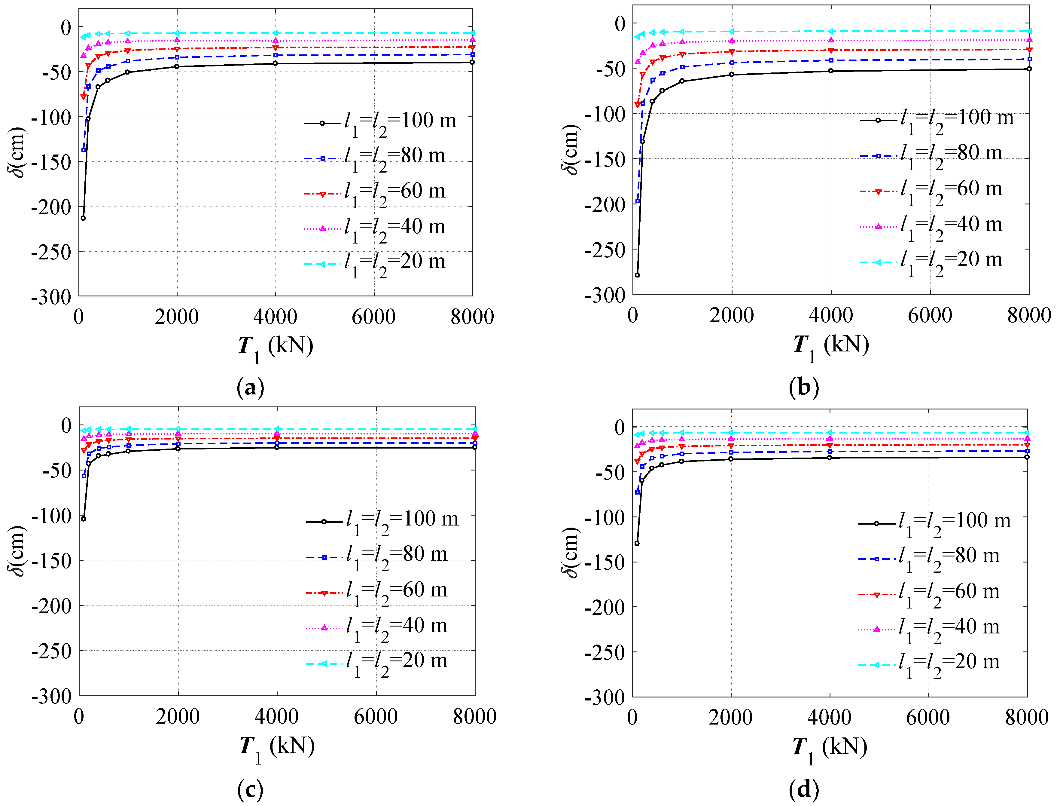
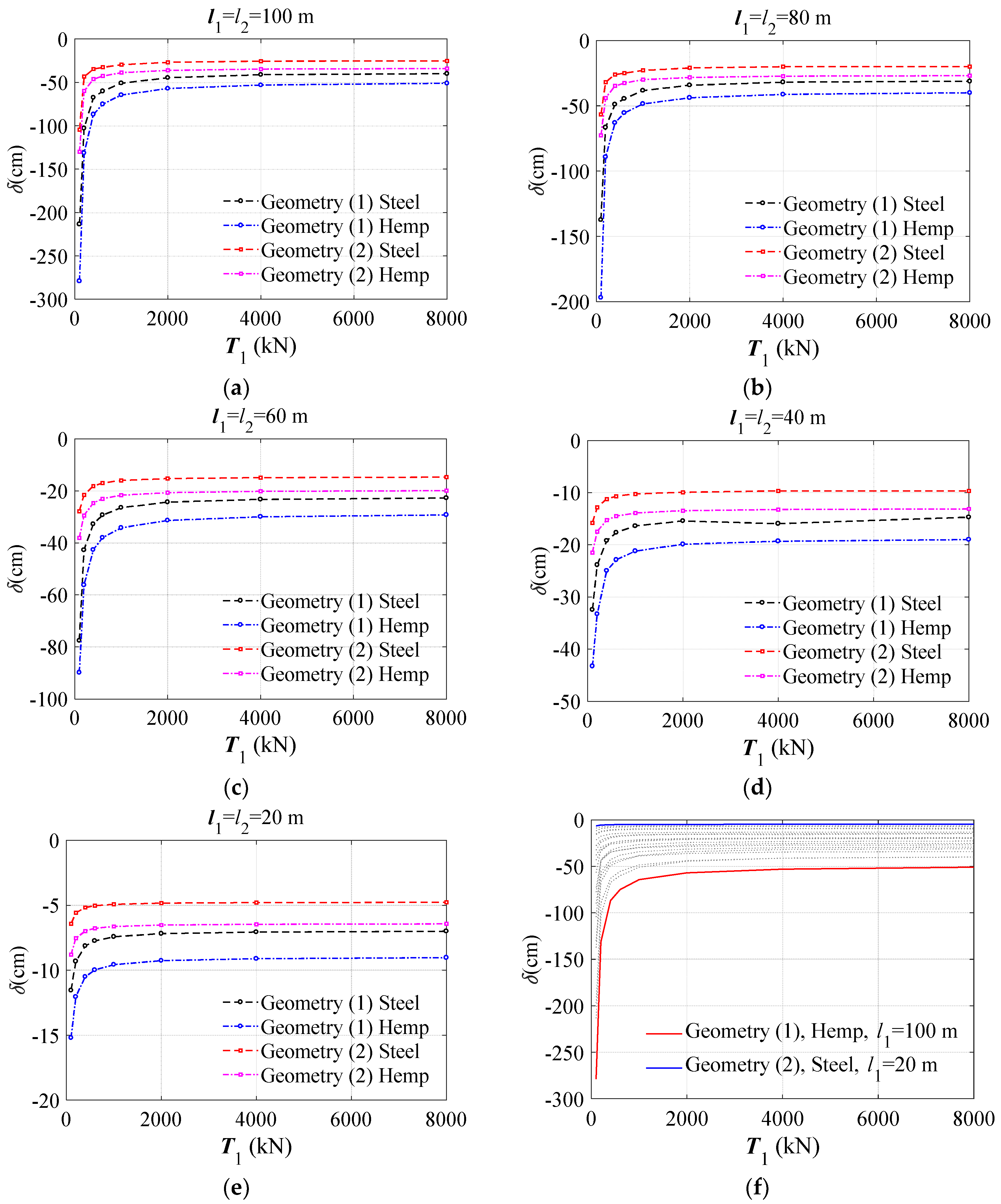
Figure 4a shows the vertical displacement trend as a function of T₁ for geometry (1) for both harmonic steel (Figure 4a) and hemp (Figure 4b) respectively, for geometry (1). Negative values of displacement mean gravitational displacements.

Static and modal analyses results have shown that the vertical displacements under dead and permanent loads (i.e., 0.5 kN/m²) vary nonlinearly as a function of load-bearing cable traction (T₁) for both harmonic steel and hemp cable nets.

Vertical displacement (i.e., in the middle of the roof), δ, tends toward very high values (i.e., in absolute value) for small values of T₁. For the smallest T₁ values (i.e., 100 kN), δ ranging from about 5/250 l₁ to 1.5/250 of l₁, for the steel cable net, and from about 7/250 l₁ to 2/250 of l₁, for the hemp cable net.

On the contrary, for the biggest T₁ value (i.e., 8000 kN), δ is constant for all plan sizes and materials, and equals about 1/250 l₁.

Similarly, for geometry (2), vertical displacement δ (Figure 4b,c) tends toward very high values for small T₁ values. However, for this geometry, the difference between steel and hemp are a minimum. In fact, for the smallest T₁ values (i.e., 100 kN), δ ranges from about 3/250 l₁ to 0.8/250 of l₁ for steel, and from about 3.3/250 of l₁ to 1.1/250 of l₁ for the hemp cable net.

The same is observed for the biggest T₁ value (i.e., 8000 kN): δ is nearly constant for all plan sizes, and it equals about 0.6/250 of l₁ for steel and 0.8/250 of l₁ for the hemp cable net.

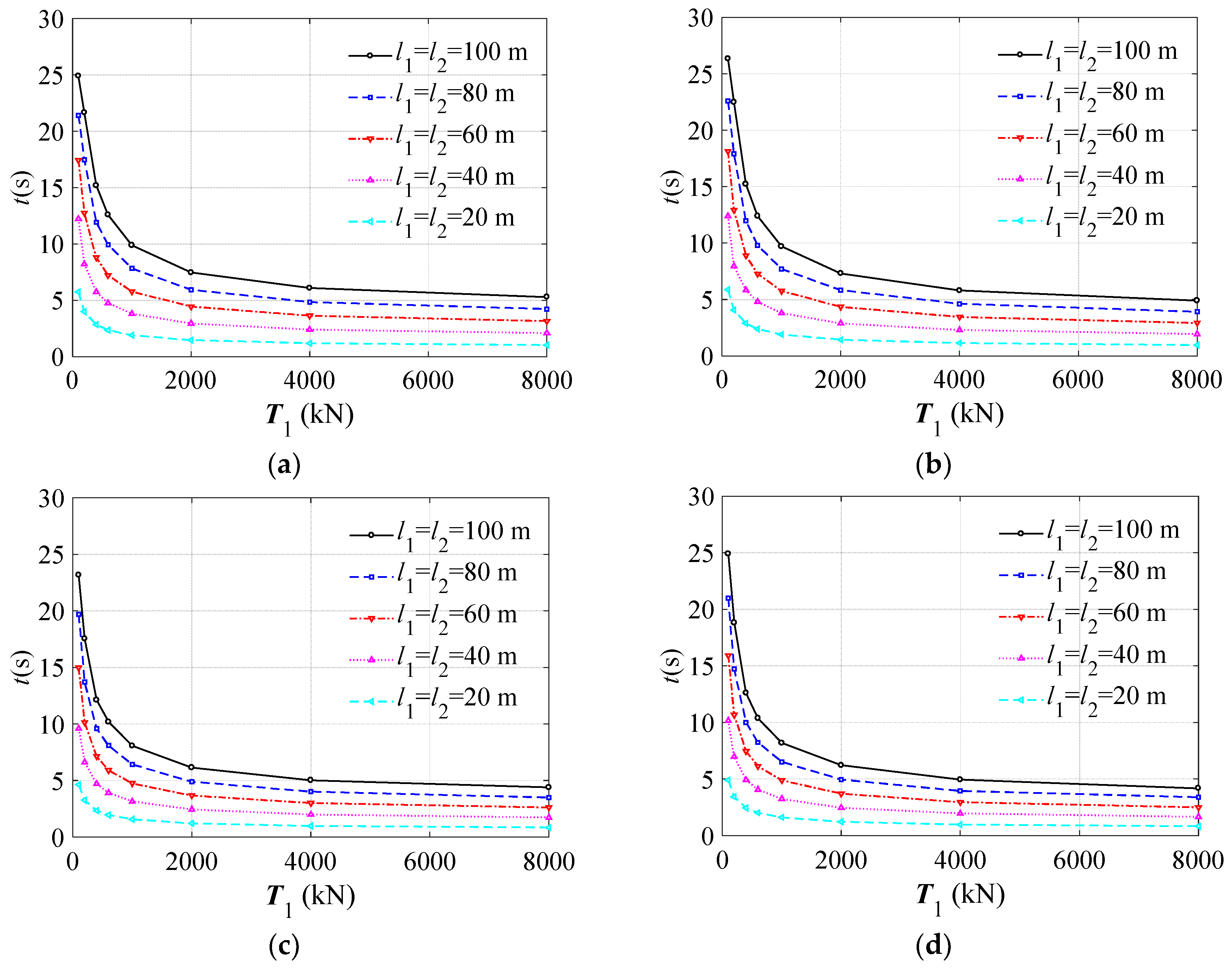
All geometries and different stiffness of the cable nets are comparable, because the cables stress limit was fixed, due to the material yield stress. Consequently, the masses varied as a function of the cable net stiffness and, so, as a function of the T₁ variation. Table 3 and Table 4 list the 1st natural frequency (ϕ) in Hz and period (t) in s values for all geometries (i.e., geometry (1) and (2), and conditions, i.e., traction, from (A) to (H)). Figure 5 synthetized the values of t as function of T₁ for both geometry (1) and (2), with harmonic steel and hemp cable nets.

Overall, except for a few cases regarding the smallest span, hemp cables had the first natural period greater than steel for both geometries and all tractions. For geometry (1), the t values ranged from 24.90 s (i.e., l₁ = 100 m and T₁ = 100 kN) to about 1.03 s (i.e., l₁ = 20 m and T₁ = 8000 kN) for steel, and from 26.33 s (i.e., l₁ = 100 m and T₁ = 100 kN) to about 0.96 s (i.e., l₁ = 20 m and T₁ = 8000 kN).

For geometry (2), the t values ranged from 23.17 s (i.e., l₁ = 100 m and T₁ = 100 kN) to about 0.85 s (i.e., l₁ = 20 m and T₁ = 8000 kN) for steel and 24.91 s (i.e., l₁ = 100 m and T₁ = 100 kN) to about 0.82 s (i.e., l₁ = 20 m and T₁ = 8000 kN).

As was expected, the first natural period of geometry (1) was slightly greater than geometry (2) for both materials used, which was due to the larger radius of curvature of the hyperbolic parabolic surface for geometry (1) than geometry (2).

With regard to steel cable nets, the standard deviation of t ranged from 5.83 s (i.e., l₁ = 100 m) to 1.05 s (i.e., l₁ = 20 m) for geometry (1), whereas it ranged from 4.66 s (i.e., l₁ = 100 m) to 0.86 s (i.e., l₁ = 20 m) for geometry (2). The standard deviation decreased when the plan sizes also decreased.

For the hemp cable net, the standard deviation of t ranged from 6.21 s (i.e., l₁ = 100 m) to 1.1 s (i.e., l₁ = 20 m) for geometry (1), whereas it ranged from 5.14 s (i.e., l₁ = 100 m) to 0.93 s (i.e., l₁ = 20 m) for geometry (2). Values of the standard deviation were lightly larger for hemp, which means that the first natural period is more sensitive, to cable stiffness and span size, than steel.

5. Remarks

The comparison between hemp and harmonic steel cable nets suggested that hemp cables have similar high performances to steel under dead and permanent load response. Obviously, results should be confirmed under extreme snow and wind action.

The weight ratio between hemp and steel is about 0.19, similarly to the Young’s modulus ratio, and contrary to the ratio between the stress limit value being about 0.25. These values suggest that hemp material is more efficient than steel in terms of the ratio weight/Young’s modulus (i.e., about 2150 for hemp and 2100 for steel) and of the stress limit/weight (i.e., about 20.2 for hemp and 15.3 for steel).

Analyses have shown that the hemp cable nets’ weight is less than steel (to obtain similar displacements and cable net stiffness), even if the hemp cable section areas are bigger than steel.

Results show that the structural response, in terms of displacements, between the two materials, is comparable for both geometries and all cable tractions considered. This means that hemp can be a valid alterative to steel. In order to show the comparison between the two materials in terms of vertical displacements and the first natural frequency obtained for all geometries, span sizes, and cable traction, Figure 6 and Figure 7 report, as follows.

Figure 6, from a to d, shows a tight similarity in trend between hemp and steel, in terms of displacements. The figure shows that geometry (2) gives smaller (in absolute value) displacements than (1) and, that for tractions greater than 2000 kN, displacements are quite constant for all geometries. Figure 6e shows a vertical displacement domain as function of the cable stiffness for designers, where the upper limit is given by geometry (2) with steel cable net, and the lower limit is given by geometry (1) with hemp cable net.

A measure of the difference between the hemp and steel cable net, in terms of displacements, is given by

Table 6. Measure ($\mathit{\delta }\mathit{d}\%$) of the vertical displacement difference between harmonic steel and hemp cable net.

Geometry	T1 (kN)	l1 (m)
		100	80	60	40	20
(1)	100	−23.5	−30.2	−13.6	−25.0	−24.0
	200	−21.7	−25.4	−24.0	−28.3	−22.7
	400	−22.4	−22.3	−23.2	−23.0	−22.6
	600	−20.0	−19.7	−22.8	−22.8	−22.4
	1000	−21.0	−21.1	−22.6	−22.8	−22.5
	2000	−21.8	−22.0	−22.5	−22.5	−22.5
	4000	−22.5	−22.7	−22.4	−17.4	−22.5
	8000	−21.7	−22.1	−22.3	−22.6	−22.5
(2)	100	−19.7	−22.0	−26.9	−26.6	−27.1
	200	−27.7	−27.5	−26.7	−26.6	−26.0
	400	−25.2	−25.0	−26.5	−26.4	−25.9
	600	−23.6	−23.6	−26.4	−26.3	−25.8
	1000	−23.8	−23.8	−26.3	−26.3	−25.8
	2000	−25.9	−26.0	−26.2	−26.3	−25.9
	4000	−26.4	−26.5	−26.2	−27.0	−25.9
	8000	−25.7	−25.8	−26.1	−26.2	−25.8

, where (as was estimated for masses in Table 5), the difference in percentage $\mathit{\delta }\mathit{d}\%$ is calculated for vertical displacements and listed in Table 6 (Equation (9)).

$$\mathit{\delta }\mathit{d}\% =\frac{{\left({\delta }_i\right)}_{steel}-{\left({\delta }_i\right)}_{hemp}}{{\left({\delta }_i\right)}_{hemp}}$$

(9)

Table 5 shows that the vertical displacements given by hemp cables range from 13.6% (i.e., geometry (1), l₁ = 60 m) to 30.2% (i.e., geometry (1), l₁ = 80 m). Most values are between 20% and 25%. Negative values mean that displacements given by the hemp cable net are greater than steel.

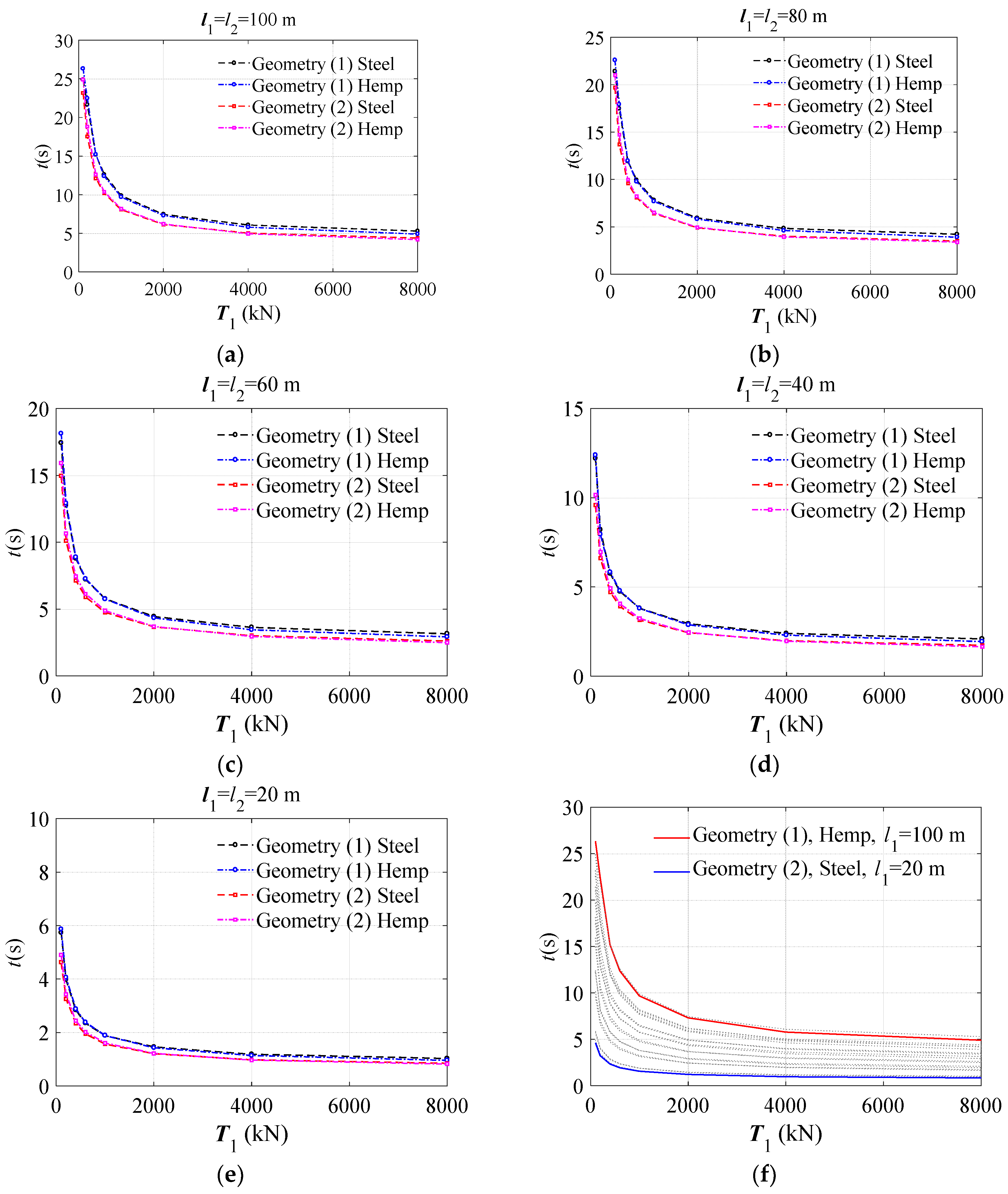
Similar to the displacement analyses, Figure 7 from a to d compares geometries, span sizes, and cable tractions between both materials, for the first natural period. The curves show a very similar trend between the materials, which suggests that, for the first natural period, the geometries affected values more than materials.

Figure 7e synthetizes the variation in a domain of the first natural period. The figures show an upper limit given by geometry (1) with the biggest span of the hemp cable net and a lower limit given by geometry (2) with the smallest span of the steel cable net.

Table 7. Measure ($\mathit{\delta }\mathit{t}\%$) of the 1st natural period difference between harmonic steel and hemp cable nets.

Geometry	T1 (kN)	l1 (m)
		100	80	60	40	20
(1)	100	−5.4	−5.2	−3.9	−1.5	−2.2
	200	−3.7	−2.5	−1.3	3.3	−2.0
	400	−0.2	−0.4	−1.0	−1.4	−1.4
	600	1.6	1.4	−0.7	−0.8	−1.3
	1000	1.9	1.7	0.4	0.3	0.0
	2000	1.9	1.9	2.3	2.1	2.1
	4000	5.0	4.8	5.2	4.4	4.4
	8000	8.0	7.9	7.9	7.7	7.3
(2)	100	−7.0	−6.2	−5.9	−5.6	−5.5
	200	−6.8	−6.9	−5.1	−4.9	−5.0
	400	−3.9	−3.9	−4.3	−4.3	−4.1
	600	−1.7	−1.7	−3.6	−3.7	−3.5
	1000	−1.3	−1.4	−2.7	−2.8	−2.5
	2000	−1.1	−1.0	−0.8	−0.4	−0.8
	4000	1.8	1.8	2.0	1.5	1.0
	8000	5.0	3.2	4.8	4.9	3.7

lists the difference percentage $\mathit{\delta }\mathit{t}\%$ calculated according to Equation (8), for the first natural period. Values are alternatively positive and negative, with a greater quantity of negative values. This means that values for hemp are mainly greater than steel. However, positive values are significant, and are focused on geometry (1) for all span sizes and for traction greater than 600 kN, while for geometry (2), for all span sizes and traction greater than 2000 kN. In this range, the hemp structures have a lower first natural period than steel, which results in a more rigid roof than for steel with the same traction. The reason is that, in this case, the cable section area size affects the results more than the global geometry (Equation (10)).

$$\mathit{\delta }\mathit{t}\% =\frac{{\left(t_i\right)}_{steel}-{\left(t_i\right)}_{hemp}}{{\left(t_i\right)}_{hemp}}$$

(10)

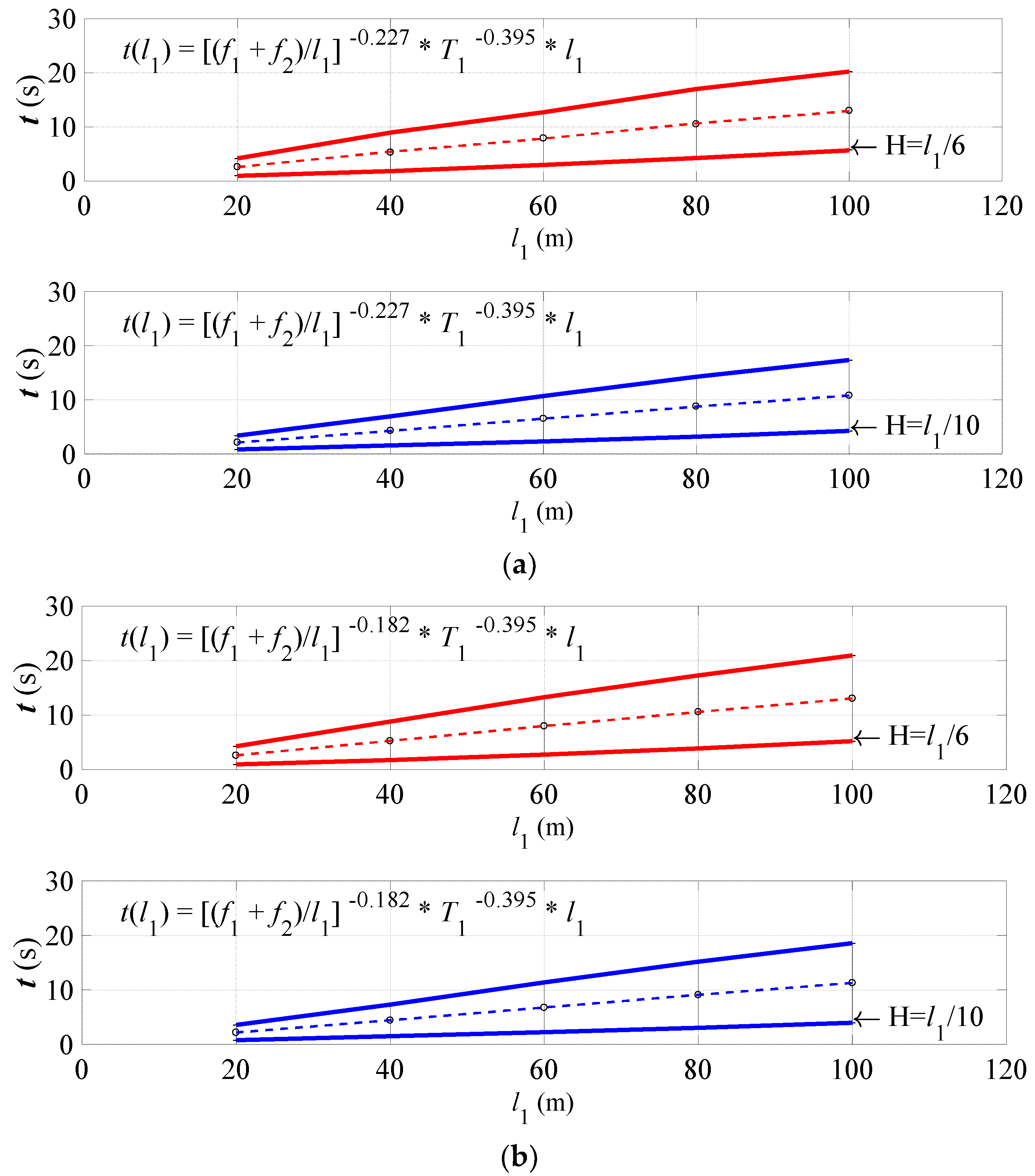
Finally, in order to give design trends of the first natural period, plan size-dependent curves are obtained, fitting the data.

Curves are illustrated in Figure 8a,b for the harmonic steel and hemp cable net, respectively. Figure 8 shows the range bars given by the estimated standard deviation obtained by varying the traction for each plan size and geometry. The range bar is slightly bigger for geometry (2) (i.e., H/l₁ = 1/6) for both materials.

The curve average is described by the function reported in Figure 8a,b.

It is important to note that the function gives a difference in percentage compared to modal analyses, with results between −7% and 6% for steel, and about −5% and 5% for hemp cable nets.

6. Conclusions

Design trends for the first natural period of hyperbolic paraboloid cable nets, with a square plan depending on span length, are given for two surfaces of hyperbolic paraboloid and two different materials for cables: harmonic steel and hemp. Two geometries of roofs are described by using two different surfaces of hyperbolic paraboloid and varying the cable sags. For each geometry, the span length was varied between 100 m and 20 m. Static and modal analyses were carried out with the aim of estimating the vertical displacements and the first natural period as a function of the cable traction and, consequently, of the cable net stiffness. The cable traction varied between 100 to 8000 kN. The comparison between hemp and harmonic steel cables showed that the two materials are comparable. Generally, hemp cables give a 20% greater vertical displacement than harmonic steel using the same cable traction. However, the difference seems acceptable considering the advantages as, for example, the sustainability, in terms of cost-benefit given by hemp cables. In addition, it is important to note that large displacements are generally accepted for these kinds of roofs. In fact, facilities, for example, are not directly connected to the roof.

The comparison between the hemp and harmonic steel cable net, regarding the first natural period, resulted in a slightly longer period for mainly hemp cables than for steel, even if for geometry (1) and for traction greater than 600 kN, the trend is opposite. The mass given by hemp cables is about, on average, 15% less than steel, even for bigger cable section areas. This result is comforting because it means that the dynamic response of these cable net systems can be very similar. The goodness of results given by hemp cable nets, encourages investigation of the wind and snow structure interaction, statically and dynamically. This goal will be developed in the next phase of the research.

References

- Herer, J. The Emperor Wears no Clothes. Text from “The Emperor Wears No Clothes” © Jack Herer. Available online: http://www.electricemperor.com/eecdrom/TEXT/TXTCH02.HTM (accessed on 1 November 2018).
- Zhang, H.; Zhong, Z.; Feng, L. Advances in the performance and application of hemp fiber. Int. J. Simul. Syst. Sci. Technol. 2016, 17. [Google Scholar] [CrossRef]
- Boesa, I.; Karus, M. The Cultivation of Hemp: Botan, Varieties, Cultivation and Harvesting; Hemptegh: Auckland, New Zealand, 1998; Volume 11, pp. 24–29. [Google Scholar]
- Cuissinat, C.; Navard, P. Swelling and dissolution of cellulose—Part III: Plant fibers in aqueous systems. Cellulose 2008, 12, 14–21. [Google Scholar] [CrossRef]
- Karus, M. Fibrin bandages include natural clotting agents—US Army and Navy tackle bleeding in different ways. Med. Text. 1999, 9, 11–13. [Google Scholar]
- Pejic, B.; Vukcevic, M.; Kostic, M.; Skundric, P. Biosorption of heavy metal ions from aqueous solutions by short hemp fibers: Effect of chemical composition. J. Hazard. Mater. 2004, 23, 152–159. [Google Scholar] [CrossRef] [PubMed]
- Mwaikambo, L.Y.; Ansell, M.P. Chemical modification of hemp, sisal, jute, and kapok fibers by alkalization. J. Appl. Polym. Sci. 2002, 84, 2222–2234. [Google Scholar] [CrossRef]
- Ouajai, S.; Shanks, R.A. Composition, structure and thermal degradation of hemp cellulose after chemical treatments. Polym. Degrad. Stab. 2005, 89, 327–335. [Google Scholar] [CrossRef]
- CGA/R. West. Published by Warner Chappell Music. Environmental and Economic Benefits of Hemp. Available online: http://www.nemeton.com/static/nemeton/axis-mutatis/hemp.html (accessed on 1 November 2018).
- Hirst, E.; Walker, P.; Paine, K.; Yates, T. Characterization of Low Density Hemp-Lime Composite Building Materials Under Compression Loading. In Proceedings of the Second International Conference on Sustainable Construction Materials and Technologies, Acona, Italy, 28–30 June 2010. [Google Scholar]
- McLaren, A.J. Design and performance of ropes for climbing and sailing. Proc. Inst. Mech. Eng. Part L J. Mater. Des. Appl. 2006, 220, 1–12. [Google Scholar] [CrossRef] [Green Version]
- Rizzo, F.; Zazzini, P. Shape dependence of acoustic performances in buildings with a Hyperbolic Paraboloid cable net membrane roof. J. Acoust. Aust. 2017, 45, 421–443. [Google Scholar] [CrossRef]
- Rizzo, F.; Zazzini, P. Improving the acoustical properties of an elliptical plan space with a cable net membrane roof. J. Acoust. Aust. 2016, 44, 449–456. [Google Scholar] [CrossRef]
- Brito, R.; Caracoglia, L. Extraction of flutter derivatives from small scale wind tunnel experiments. In Proceedings of the 11th Americas Conference on Wind Engineering, American Association for Wind Engineering (AAWE), San Juan, Puerto Rico, 22–26 June 2009. [Google Scholar]
- Rizzo, F.; Caracoglia, L.; Montelpare, S. Predicting the flutter speed of a pedestrian suspension bridge through examination of laboratory experimental errors. Eng. Struct. 2018, 172, 589–613. [Google Scholar] [CrossRef]
- Rizzo, F.; Caracoglia, L. Examining wind tunnel errors in Scanlan derivatives and flutter speed of a closed-box. J. Wind Struct. 2018, 26, 231–251. [Google Scholar]
- Avossa, A.M.; Di Giacinto, D.; Malangone, P.; Rizzo, F. Seismic retrofit of a multi-span prestressed concrete girder bridge with friction pendulum devices. Shock Vib. 2018. [Google Scholar] [CrossRef]
- Boggs, D.; Lepage, A. Wind Action on Structures—D.3 Wind Tunnel Testing Procedures; 4354:2012(E); ISO (International Standards Organization): Geneva, Switzerland, 2012. [Google Scholar]
- American Society of Civil Engineering (ASCE). Wind Tunnel Studies of Buildings and Structures; Isyumov, N., Ed.; Manuals of Practice (MOP) 67; ASCE: Reston, VA, USA, 1999. [Google Scholar]
- American Society of Civil Engineering (ASCE). Minimum Design Loads for Buildings and Other Structures; ASCE 7:2010; ASCE: Reston, VA, USA, 2010. [Google Scholar]
- NRC/CNRC (National Research Council/Conseil National de Recherches Canada). Commentary to the National Building Code of Canada; Commentary I: Wind Load and Effects; NRC/CNRC: Ottawa, ON, Canada, 2010. [Google Scholar]
- Architectural Institute of Japan (AIJ). Recommendations for Loads on Buildings, Chapter 6: Wind Loads; AIJ: Tokyo, Japan, 2004. [Google Scholar]
- Swiss Society of Engineers and Architects (SIA). Action on Structures—Appendix C: Force and Pressure Factors for Wind; SIA 261:2003; SIA: Zurich, Switzerland, 2003. [Google Scholar]
- Standards Australia (AS); Standards New Zealand (NZS). Structural Design Actions; Part 2: Wind Actions, AS/NZS 1170.2:2002; Standards Australia: Sydney, Australia; Standards New Zealand: Wellington, New Zealand, 2011.
- Krishna, P.; Kumar, K.; Bhandari, N.M. Wind Loads on Buildings and Structures; Indian Standard IS:875, Part 3; Proposed Draft & Commentary; Bureau of Indian Standards: Delhi, India, 2012.
- Comité Européen de Normalization (CEN). Eurocode 1: Actions on Structures—Part 1–4: General Actions—Wind Actions; EN-1991-1-4; Comité Européen de Normalization: Brussels, Belgium, 2005. [Google Scholar]
- National Research Council of Italy (CNR). Guide for the Assessment of Wind Actions and Effects on Structures; CNR-DT 207/2008; CNR: Roma, Italy, 2008. [Google Scholar]
- Vassilopoulou, I.; Gantes, C.J. Nonlinear dynamic behavior of saddle form cable nets under uniform harmonic load. Eng. Struct. 2011, 33, 2762–2771. [Google Scholar] [CrossRef]
- Vassilopoulou, I.; Gantes, C.J. Vibration modes and natural frequencies of saddle form cable nets. Comput Struct. 2012, 88, 105–119. [Google Scholar] [CrossRef]
- Vassilopoulou, I.; Petrini, F.; Gantes, C.J. Nonlinear dynamic behavior of cable nets subjected to wind loading. Structures 2017, 10, 170–183. [Google Scholar] [CrossRef]
- Majowiecki, M. Tensostrutture: Progetto e Verifica; Edizioni Crea: Massa, Italy, 1994. [Google Scholar]
- Rizzo, F.; Sepe, V. Static loads to simulate dynamic effects of wind on hyperbolic paraboloid roofs with square plan. J. Wind Eng. Ind. Aerodyn. 2015, 137, 46–57. [Google Scholar] [CrossRef]
- Daw, D.J.; Davenport, A.G. Aerodynamic damping and stiffness of a semi-circular roof in turbulent wind. J. Wind Eng. Ind. Aerodyn. 1989, 32, 83–92. [Google Scholar] [CrossRef]
- Forster, B. Cable and membrane roofs, a historical survey. Struct. Eng. Rev. 1994, 6, 3–5. [Google Scholar]
- Kassem, M.; Novak, M. Wind-Induced response of hemispherical air-supported Structures. J. Wind Eng. Ind. Aerodyn. 1992, 41, 177–178. [Google Scholar] [CrossRef]
- Knudson, W.C. Recent advances in the field of long span tension structures. Eng. Struct. 1991, 13, 174–193. [Google Scholar] [CrossRef]
- Letchford, C.W.; Killen, G.P. Equivalent static wind loads for cantilevered grandstand roofs. Eng. Struct. 2002, 24, 207–217. [Google Scholar] [CrossRef]
- Letchford, C.W.; Denoon, R.O.; Johnson, G.; Mallam, A. Dynamic characteristics of cantilever grandstand roofs. Eng. Struct. 2002, 24, 1085–1090. [Google Scholar] [CrossRef]
- Lewis, W.J. Tension Structures: Form and Behavior; Thomas Telford: London, UK, 2003. [Google Scholar]
- Pun, P.K.F.; Letchford, C.W. Analysis of a tension membrane HYPAR roof subjected to fluctuating wind loads. In Proceedings of the 3rd Asia-Pacific symposium on Wind Engineering, Hong Kong, China, 13–15 December 1993; University of Hong Kong: Hong Kong, China, 1993; pp. 741–746. [Google Scholar]
- Shen, S.; Yang, Q. Wind-induced response analysis and wind-resistant design of hyperbolic paraboloid cable net structures. Int. J. Space Struct. 1999, 14, 57–65. [Google Scholar] [CrossRef]
- Yang, Q.; Liu, R. On Aerodynamic Stability of Membrane Structures. Int. J. Space Struct. 2005, 20, 181–188. [Google Scholar] [CrossRef]
- Yang, Q.; Wu, Y.; Zhu, W. Experimental study on interaction between membrane structures and wind environment. Earthq. Eng. Eng. Vib. 2010, 9, 523–532. [Google Scholar] [CrossRef]
- Biagini, P.; Borri, C.; Facchini, L. Wind response of large roofs of stadiums and arena. J. Wind Eng. Ind. Aerodyn. 2007, 95, 9–11. [Google Scholar] [CrossRef]
- Dong, X.; Ye, J.H. Development and verification of a flow model of conical vortices on saddle roofs. J. Eng. Mech. 2015, 141, 04014127. [Google Scholar] [CrossRef]
- Elashkar, I.; Novak, M. Wind tunnel studies of cable roofs. J. Wind Eng. Ind. Aerodyn. 1983, 13, 407–419. [Google Scholar] [CrossRef]
- Kawai, H.; Yoshie, R. Wind-induced response of a large cantilevered roof. J. Wind Eng. Ind. Aerodyn. 1999, 83, 263–275. [Google Scholar] [CrossRef]
- Kawakita, S.; Bienkiewicz, B.; Cermak, J.E. Aeroelastic Model Study of Suspended Cable Roof. Fluid Mechanics and Wind Engineering Program; Department of Civil Engineering, Colorado State University: Fort Collins, CO, USA, 1992. [Google Scholar]
- Sykes, D.M. Wind loading tests on models of two tension structures for EXPO’92, Seville. J. Wind Eng. Ind. Aerodyn. 1994, 52, 371–383. [Google Scholar] [CrossRef]
- Irwin, H.P.A.H.; Wardlaw, R.L.A. Wind tunnel investigation of a retractable fabric roof for the Montreal Olympic stadium. In Proceedings of the 5th International Conference on Wind Engineering, Fort Collins, CO, USA, 8–14 July 1979; pp. 925–938. [Google Scholar]
- Sun, X.; Wu, Y.; Yang, Q.; Shen, S. Wind tunnel tests on the aeroelastic behaviors of tension structures. In Proceedings of the VI International Colloquium on Bluff Bodies Aerodynamics & Applications, BBAA VI, Milan, Italy, 20–24 July 2008. [Google Scholar]
- Rizzo, F.; D’Asdia, P.; Ricciardelli, F.; Bartoli, G. Characterization of pressure coefficients on hyperbolic paraboloid roofs. J. Wind Eng. Ind. Aerodyn. 2012, 102, 61–71. [Google Scholar] [CrossRef]
- Rizzo, F. Wind tunnel tests on hyperbolic paraboloid roofs with elliptical plane shapes. Eng. Struct. 2012, 45, 536–558. [Google Scholar] [CrossRef]
- Killen, G.P.; Letchford, C.W. A parametric study of wind loads on grandstand roofs. Eng. Struct. 2001, 23, 725–735. [Google Scholar] [CrossRef]
- Rizzo, F.; Ricciardelli, F. Design pressure coefficients for circular and elliptical plan structures with hyperbolic paraboloid roof. J. Eng. Struct. 2017, 139, 153–169. [Google Scholar] [CrossRef]
- Kimoto, E.; Kawamura, S. Aerodynamic criteria of hanging roofs for structural Design. In Proceedings of the IASS Symposium, Osaka, Japan, 15–19 September 1986; pp. 249–256. [Google Scholar]
- Rizzo, F.; Barbato, M.; Sepe, V. Peak factor statistics of wind effects for hyperbolic paraboloid roofs. Eng. Struct. 2018, 173, 313–330. [Google Scholar] [CrossRef]
- Liu, M.; Chen, X.; Yang, Q. Characteristics of dynamic pressures on a saddle type roof in various boundary layer flows. J. Wind Eng. Ind. Aerodyn. 2016, 150, 1–14. [Google Scholar] [CrossRef]
- Rizzo, F. Tensile Structures of Cables Net, Guidelines to Design and Applications. Open J. Civ. Eng. 2016, 6. [Google Scholar] [CrossRef]
- Rizzo, F.; D’Asdia, P.; Lazzari, M.; Procino, L. Wind action evaluation on tension roofs of hyperbolic paraboloid shape. Eng. Struct. 2011, 33, 445–461. [Google Scholar] [CrossRef] [Green Version]
- Vadivambal, R.; Vellaichamy, C.; Jian, F.; Jayas, D. Tensile strength and elongation of hemp and sisal ropes at different temperatures. Can. Biosyst. Eng. 2015, 57, 3.9–3.12. [Google Scholar] [CrossRef]
- Berr, J. International Directory of Hemp Products & Suppliers; The Message Company: Paris, France, 1996; Volume 23, pp. 74–85. [Google Scholar]
- Keller, A. Compounding and mechanical properties of biodegradable hemp fiber composites. Compos. Sci. Technol. 2003, 63, 1307–1316. [Google Scholar] [CrossRef]
- Robinson, R. The Great Book of Hemp; Park Street Press: Rochester, UK, 1996; Volume 21, pp. 54–65. [Google Scholar]
Figure 1.
Geometrical parameters (a) geometry (1), (b) geometry (2).
Figure 2.
The cables connection (a), the cable net model: the “Rope-beam” model (b).
Figure 3.
Examples of FEM models: geometry (1) (a) and (2) (b) with span equal to 100 m, example of the 1st modal shaped for all different geometries (c).
Figure 4.
Vertical displacements under dead and permanent loads depending on cable traction, geometry (1) harmonic steel (a) and hemp (b); geometry (2) harmonic steel (c) and hemp (d).
Figure 5.
1st natural period dependence on cable traction, geometry (1) harmonic steel (a) and hemp (b); geometry (2) harmonic steel (c) and hemp (d).
Figure 6.
Comparison between harmonic steel and hemp: vertical displacement dependence on cable traction from l1 = l2 = 100 m (a), 80 m (b), 60 m (c), 40 m (d), 20 m (e); variation domain (f).
Figure 7.
Comparison between harmonic steel and hemp: 1st natural period dependence on cable traction from l1 = l2 = 100 (a), 80 m (b), 60 m (c), 40 m (d), 20 m (e); variation domain (f).
Figure 8.
Prediction design trends of the 1st natural period as function of geometry (red = 1, blue = 2): harmonic steel (a) and hemp (b) cable nets.