A Method for Fast Selection of Machine-Learning Classifiers for Spam Filtering

Abstract

The paper elaborates on how text analysis influences classification—a key part of the spam-filtering process. The authors propose a multistage meta-algorithm for checking classifier performance. As a result, the algorithm allows for the fast selection of the best-performing classifiers as well as for the analysis of higher-dimensionality data. The last aspect is especially important when analyzing large datasets. The approach of cross-validation between different datasets for supervised learning is applied in the meta-algorithm. Three machine-learning methods allowing a user to classify e-mails as desirable (ham) or potentially harmful (spam) messages were compared in the paper to illustrate the operation of the meta-algorithm. The used methods are simple, but as the results showed, they are powerful enough. We use the following classifiers: k-nearest neighbours (k-NNs), support vector machines (SVM), and the naïve Bayes classifier (NB). The conducted research gave us the conclusion that multinomial naïve Bayes classifier can be an excellent weapon in the fight against the constantly increasing amount of spam messages. It was also confirmed that the proposed solution gives very accurate results.

1. Introduction

The spam problem is an ongoing issue: in 2018 14.5 billion spam e-mails were sent per day [1]. According to the Internet Security Threat Report [2] released in 2019 by Symantec, spam levels for their customers increased in 2018. What draws the attention is that small enterprises were attacked more often than large companies, and e-mail malware reached stable levels. Therefore, there is a need to tailor even simple tools for detection and filtering of spam in all organizations.

For the sake of the presented study, we follow the definition by Emilio Ferrara, stating that this is any “attempt to abuse, or manipulate, a techno-social system by producing and injecting unsolicited and/or undesired content aimed at steering the behavior of humans or the system itself, at the direct or indirect, immediate or long-term advantage of the spammer(s)” [3]. Here, we focus on so-called junk e-mails. These are unwanted messages sent at large scale by e-mail. The term spam refers to the undesired (or even harmful) e-mails, while ham is used to indicate the valid and important messages desired by the recipient. Additionally, we assume the scenario where junk e-mails are sent by botnets and they are not aimed at specific users (contrary to, e.g., spear phishing).

This paper proposes a method for identification of the best-performing machine-learning-based classifiers and selection of the one with the leading parameters. The proposed solution solves the problem of fast recognition of the most interesting parameters. This allows for quick analysis of data of higher dimensionality. This is especially important if large datasets are to be analyzed and we want to assure the proper scalability of our system. In our paper, we also show how to find a database to train a machine-learning model used for spam detection (defined here as a binary classifier), to process the text so that the data can be fed to a machine-learning model and how to implement a selected machine-learning model-based classifier. We also propose a method that allows for cross-validation between different datasets in the training and test phases. The obtained results show that our solution gives accurate results consistent with other literature studies and outperforms the reported results in some cases. To the best of our knowledge, our paper is the first which discusses the efficiency of SVM, MNB, k-NN algorithms for such comprehensive datasets as almost the whole Enron (4 datasets) and Lingspam databases. Moreover, it uses an unusual cross-validation concept by mixing and applying different datasets for training and test purposes. Such an approach is extremely rare in the literature. Finally, it presents a multistage algorithm for fast and precise selection of machine-learning classifiers for spam filtering. It allows for quick selection of interesting parameters, which is essential for working with large datasets. The quality of the results is proven by a big numerical example given for the method validation.

The structure of the paper is as follows. The review of spam filters based on different machine-learning tools with typical performance metrics and several publicly available datasets is presented in Section 2. In Section 3, the materials and methods are discussed. The assumptions, useful databases of spam messages, text-preprocessing aspects (including tokenization, conversion, removal of punctuation marks, stemming/lemmatization, and dictionary construction) as well as the considered supervised learning solutions are described. The performance of the selected methods is evaluated on four large datasets in Section 4. The dataset structures created with the unique approach of assuring cross-validation between different datasets in training and test phases are analyzed first. Next, the text preprocessing impact on the used dictionary is studied. An innovative multistage meta-algorithm for checking the classifier performance is described in action and validated. The final summary is given in Section 5.

2. Related Work

The increasing number of spam e-mails has created a strong need to develop more reliable and efficient anti-spam filters, including ones based on machine-learning tools. They are efficient, since they only require the preparation of a set of training samples, i.e., pre-classified e-mails [4]. In recent years, various machine-learning methods have been successfully used to effectively detect and filter unwanted messages. The following classification methods are most commonly used for spam filtering: Support Vector Machine (SVM), Naïve Bayes classifier (NB), k-Nearest Neighbours (k-NN), Artificial Neutral Network (ANN), Decision Tree (DT), Random Forest (RF), Logistic Regression (LR). Below, we present some results reported in the literature. Note that some of the metrics results are compared with our method during the validation of our approach. The values are given at the end of the numerical study in separate table.

The applicability of using different machine-learning methods to recognize spam e-mails was analyzed in [5]. The SpamAssassin dataset, which contains 6000 e-mails with the spam rate 37.04% used in all experiments. Sharma and Arora in [6] analyzed Bayes Net (BN), Logic Boost (LB), RT, JRip (JR), J48-based DTs, Multilayer Perceptron (MP), Kstar (KS), RF, and Random Committee (RC) machine-learning algorithms. The dataset with 4601 instances and 55 spam base attributes downloaded from UCI Machine-Learning Repository were used in the performed research. Harisinghaney et al. [7] applied the following three different algorithms: k-NN, NB, and DBSCAN-based clustering. The performance for the four metrics accuracy, precision, sensitivity, and specificity were calculated and compared. Unfortunately, contrary to our approach, only a small set of the Enron Corpus dataset was used in the analysis (2500 mails for training and another 2500 mails for testing from 200,399 messages of the cleaned Enron Corpus). In [8] a comprehensive study of machine-learning mechanisms for spam mail detection such as NB, SVM, and k-NN combined with NB is presented. The TREC 2007 public corpus with 12 attributes and 4899 messages as the spam base dataset was used for performance evaluation. The accuracy and F-measure were calculated and compared for all algorithms. The authors in [9] prepared a special dataset called SHED: Spam Ham E-mail Dataset. They collected 6002 e-mails (4490 spam and 1512 ham e-mails) and extracted from them various features. The performance of different classification approaches (NB, BN, AdaBoost, and RF) was evaluated using four metrics: accuracy, precision, recall, and time taken to build the model. In [10] the NB, SVM and hybrid solutions were studied using Lingspam dataset. The authors observed that the SVM algorithm in most cases offers high precision and recall, while NB offers faster classification speed. They also require fewer training samples. The authors in [11] showed how to develop a high-performance and low-computation method for classifying spam e-mails. The UCI SpamBase dataset was used with a total of 4601 data instances for experimentation. The following classifiers were evaluated and compared: RF, ANN, Logistic, SVM, Random Tree, k-NN, Decision Table, BN, NB, and neural networks applying Radial Basis Functions (RBF). Seven metrics were used to evaluate the performance of the classifiers. In [12], another comparison between different machine-learning classifiers was presented. The classifiers analyzed in this paper include SVM, NB, and J48. The dataset used in this research was enron1 from the Enron collection of e-mails. It contained 3762 spam messages and 5172 ham messages. The performance analysis of seven machine-learning techniques for e-mail spam classification was analyzed in [13]. The following techniques were compared: NB, SVM, k-NN, RF, Bagging, Boosting (AdaBoost), and Ensemble Classifier. The evaluation was performed on the e-mail spam dataset from UCI Machine-Learning Repository and Kaggle website. In [14], the problem of spam review detection is addressed. The authors proposed in their system deep-learning methods: Multilayer Perceptron (MLP), Convolutional Neural Network (CNN), and a variant of Recurrent Neural Network (RNN) based on Long Short-Term Memory (LSTM) cells. They also applied traditional classifiers such as NB, k-NN and SVM. They worked on Ott and Yelp Datasets in their study. The presented results showed that considering accuracy, both SVM and NB classifiers performed almost same. The problem of spam and malware elimination from e-mails was discussed in [15]. The authors analyzed and compared ten classification techniques: k-NN, SVM, DT, RF, AdaBoost, Extra Tree (ET), Gaussian Naïve Bayes (GNB), Multinomial Naïve Bayes (MNB), Bernoulli Naïve Bayes (BNB), and Gradient Boosting (GB). These algorithms were trained on previously labeled data from the shortened Enron and CMU datasets (26,000 spam and 19,000 ham e-mails) and the accuracy of each classifier was computed. The SVM obtained the best results. We would like to emphasise that—although we also compare some classifiers—our main aim is to propose a general meta-algorithm to deal with various classifiers. This differs us from works such as [15].

Guarav et al. [16] examined the efficiency of NB, DT, and RF algorithms used in the classification process. The experiments were carried out on three different types of datasets: Lingspam, Enron and PU. In the comparative study, the authors showed that the accuracy level for all algorithms highly depended on a specific dataset. In [17] the four classifiers: NB, DT, Ensemble Boosting and Ensemble Hybrid Boosting (EHB) were analyzed and compared. The authors used UCI Machine-Learning Repository as a spam dataset. The mentioned dataset has 4601 instances, 57 attributes, and a single output which allows classification of e-mail as spam or ham. A large group of machine-learning techniques for e-mail spam classification was also analyzed and presented in [18]. The authors studied the efficiency of the following algorithms: SVM, k-NN, NB, DT, RF, AdaBoost and Bagging. They used e-mail data sets from different websites, such as Kaggle, along with some datasets created on their own. A spam e-mail dataset from Kaggle was used for training. The performed research showed that the NB gave the best results, but expressed a limitation due to class-conditional independence. Gibson et al. [19] analyzed machine-learning algorithms that are optimized with bio-inspired methods. They implemented Multinominal Naïve Bayes (MNB), SVM, RF, DT, and Multilayer Perceptron algorithms which were tested on seven different e-mail datasets: Lingspam, PUA, PU1, PU2, PU3, Enron, and SpamAssassin. The bio-inspired algorithms such as Particle Swarm Optimization (PSO) and Genetic Algorithm (GA) were added for performance optimization of classifiers. The GA worked well for RF and DT, whereas PSO worked well for MNB. The authors proved that MNB with GA performed the best overall. In [20], three techniques, namely NB, k-NN and SVM, were studied on a prepared dataset. The corpus consists of 16,843 messages, 11,291 of which are marked as spam (from the Babletext web site) and 5552 are labeled as ham (from the SpamAssassin web site). The best accuracy was obtained for NB. The authors in [21] compared: Logistic Regression (LR), DT, NB, k-NN, and SVM as the classifiers. The assumed dataset was a spam database taken from UCI Machine-Learning Repository. The RD and k-NN obtained the same performance; however, k-NN algorithm requires more time to build the model. The accuracy of both algorithms exceeded 99%. Saidini et al. [22] explored the use of a semantic-based classification approach to improve the accuracy of spam detection. The NB, k-NN, DT, AdaBoost, and RF machine-learning classifiers were compared in terms of accuracy, recall, precision, and F-measure. The test dataset was collected from several public sources: Enron, Lingspam and some specialized forums. To extend the evaluation part, the authors also used another dataset, called CSDMC2010. They noted that NB and SVM performed better than the other tested classifiers. The categorization by domain significantly improved the spam detection process. The best results were obtained using AdaBoost, NB, and RF classifiers, where the accuracy achieved more than 98% in most of domains. In [23], the authors implemented MNB, RF, k-NN, GB, as well as RNN and MLP for deep-learning implementation. The dataset with 4601 instances (1813 spam and 2788 non-spam messages) from the UCI Machine-Learning Repository was applied for analysis. Rastenis et al. [24] proposed an automated spam and phishing e-mail classification solution, which is based on e-mail message body text automated classification. It also solves the problem of correct classification of e-mails written in different languages. They compared NB, General Linearized Model (GLM), Fast Large Margin (FLM), DT, RF, GB, and SVM on Nazario, SpamAssassin, and Vilnius Technical University datasets. Records from different datasets were mixed into one reduced dataset (700 spam and 700 phishing e-mails).

Although we focus here on the usage of many classifications simultaneously, it can be mentioned that a large part of the literature is devoted to the analysis of one type of model to classify e-mails (e.g., [25]) or the potential attacks on classification tasks (such as for instance in [26]). Additionally, it is necessary to remember that some works report that although it is evident that algorithms that perform well in the spam classification (e.g., NB), in other contexts they offer poor performance (e.g., [27,28]). Therefore, the model should always be aligned with a specific problem and data type.

3. Materials and Methods

3.1. Assumptions

E-mail spam filtering is a compound task, and in general we follow the methods elaborated before, where [29] is the main source of inspiration for us. The main goal of this paper is to explore one of its key areas, i.e., machine-learning-based classification, to help with the initial decision if a given e-mail message is indeed spam or ham. The element that enables this research is a dataset selected as a pool for training. The dataset is a collection of real e-mail examples. Access to a useful dataset is not a trivial issue, since typically in the academical world it is not possible to obtain e-mails for scientific research. Additionally, it is necessary to gain access to the database where the messages are already labeled as spam or ham.

Here, we propose a multistage meta-algorithm that allows us to select the best hyperparameters for various classification algorithms and then compare their performance to decide on which one to use. The meta-algorithm is presented in Figure 1. Please note that the classification algorithms shown are only used as illustration. The following stages of the meta-algorithm are as follows:

• Selection of a database.
• Text analysis.
• Spam detection: cross-validation on different datasets.
• Final selection.

These elements are presented in the subsequent part of the paper. As for now, we can emphasise that our approach deals mainly with the impact the text preprocessing has on the classification process and then analyzes illustratively some of the machine-learning methods performance in this difficult task. Our solution consists of two parts. The first one focuses on the text documents (e-mails) analysis and preprocessing (points 1 and 2 above), so that the documents can be represented as an input for the methods used afterwards. The second one (points 3 and 4 above) implements the classifiers and provides the tools to evaluate them. First, we present the selection of the database (assumptions in Section 3.2 and their concretization in Section 4.1) to obtain the samples to train, adjust, validate, and test any model. Second, we elaborate on how to process the dataset to make it usable for various models and valuable enough to provide meaningful data. As in many cases, data processing (along with feature selection) is important since the quality strongly depends on it. The assumptions behind the text analysis are discussed in Section 3.3, while the details related to concrete data are shown in Section 4.2. Third, the main part of the method is performed in a few substages (five in our example case), and assures the proper scalability of the system. It consists mainly in the preselection of the classifiers and adjustment of their hyperparameters. The concept lays in the fact that the largest number of tests is conducted on the smallest dataset. This approach allows us to obtain the most interesting parameters relatively quickly, and then proceed to check them on data of higher dimensionality. The exemplary classifiers are shortly refreshed in Section 3.4. We emphasise that these models are used only to illustrate our method. All substages are thoroughly shown in the numerical example (Section 4.3). Fourth, as concerns the final selection, we just present the comparison of the output in Section 4.4. The selection should be performed based on a specific application or user’s needs, and we do not settle these concerns here.

As can be seen, the proposed meta-algorithm does not solve any specific machine-learning problem, but is a kind of super-algorithm able to select the best algorithms to solve classification problems. As concerns the complexity of the meta-algorithm, we can see that it does not involve any loops or recurrences, so it is purely linear and, therefore, its scalability is very good. In fact, the only elements that can increase the complexity are related to its elements. Potentially problematic stages are related to text analysis, but is it necessary to mention that tokenization, lemmatization, stemming, etc. operate linearly from the viewpoint of the dataset size and its efficiency is mainly related to the search mechanisms involved. As we are using the mechanisms built in the popular machine-learning package, we do not consider their internal complexity. Clearly, a problematic part of the calculations can be also related to the models themselves. Although it is known that the pessimistic complexity of the used classification algorithms (k-NNs, NBs, SVMs) is in general polynomial (no larger than cubic—even in the case of naive implementations), we additionally purposely limit the calculation time by cutting the hyperparameter and training processing times by fast skipping of the models with poor performance based on the training sets with increasing size and complexity. In practice, our experiments were done on a standard desktop PC and the processing time has not exceeded standard times reported in the literature.

3.2. Databases

The first issue to solve while dealing with e-mail spam filtering is to find a dataset needed to train and test the models. It is extremely difficult to find a useful dataset of this kind. Although the total number of e-mails sent/received worldwide in 2019 was expected to reach 293.6 billion [30] per day, the access to the data is hindered due to privacy issues. We had to use publicly accessible data that are free and open to the whole world, which diminishes the set of potential candidates. Additionally, we were interested in databases conforming the following properties: (a) accessible: public and free to download for academic purposes; (b) relatively new: the old databases are not useful since the spamming environment is extremely dynamic; (c) virus-free. During the research, a few sources were selected. Their short descriptions are given below.

• Enron Corpus: chosen to be a foundation for this paper. The corpus is described in detail in the following.
• Lingspam: a part of the database (962 e-mails) was preprocessed and used by Gregory Piatetsky-Shapiro and Matthew Mayo in their implementation of e-mail spam filtering [29]. The dataset was also downloaded and used in our experiments.
• SpamAssassin (SA): a public corpus which was last updated in 2006 [31]. SA is an open-source anti-spam platform [32], filtering e-mail and blocking spam. The tests are carried out on e-mail headers and bodies.
• Honeypot: the last event entered in the website is up to date. Honeypot gathers statistics about harvesters, spam servers, dictionary attackers, and comment spammers. The owners claim that they “periodically collate the e-mail messages they receive and share the resulting corpus with anti-spam developers and researchers” [33]. Unfortunately, they do not provide any ham e-mails.
• MailBait: fills the inbox with e-mails by signing up the provided address for mailing lists and newsletters [34]. It is not anonymised (browser data and IP pass through) and it does not provide ham.

The Enron Corpus [35] was collected at Enron Corporation in 2002, during the investigation after the bankruptcy of the company. The original set was generated by 158 employees and consists of more than 600,000 e-mails. This database has already been used in the studies on machine-learning-based spam detection [36]. The corpus consists of two subdirectories: the ‘raw’ one (original messages with no modifications) and the ‘preprocessed’ one (where the messages in non-Latin encoding, virus-infected e-mails and ham sent by the owners to themselves were removed).

3.3. Processing of the Data

Text preprocessing plays a crucial role in spam filtering [24,37]. For any spam detection model to be effective, the content of the e-mails should be normalized and represented as feature vectors. The starting point is the tokenization of the raw text data. Then there are several steps shown in Figure 2 to obtain the data in the form that is ready to be analyzed by the model.

Tokenization technique allows us to split the content of the e-mails into basic processing units that are called tokens or features. Given that the paper deals with text data, the tokens are simply separate words. For instance, the tokenized sentence “Subject: christmas tree farm pictures” is a collection of strings: “Subject”, “:”, “christmas”, “tree”, “farm” and “pictures”. The next step involves converting all tokens to lowercase. As a result of this simple operation, the number of words taken into account is significantly reduced. Instead of treating “Example”, “example” and “EXAMPLE” as three different words, after converting them to lowercase, we make sure that the program will count them as one (“example”). Punctuation marks, digits, and stop words are all common in both spam and ham e-mails and do not add any value to text analysis. Since we implement our solution in Python, we refer to tools related to this programming language. There are several libraries and functions that may be applied to eliminate the mentioned language elements not essential from the spam detection viewpoint. Below is the list of functionalities chosen by us.

• Python method string.isalpha() checks whether the characters in the string are alphabetic or not. If the character is a digit, the method returns False.
• The method string.punctuation() allows removal of common punctuation marks, such as commas, periods, semicolons, etc.
• Natural Language Toolkit (NLTK) offers a module containing a list of stop words that are the most common words in a language. The examples of stop words are short words, for example: “the”, “is”, “at”, “which”, or “on” [38]. The universal list of stop words does not exist, any set can be adopted depending on the purpose.

Next, stemming reduces the morphological variants of the word to its base (stem). The algorithms enabling that operation are often called stemmers. In Python, that may be implemented with the use of NLTK [39]. For English language, there exist two stemmers: PorterStemmer and LancasterStemmer. For the purpose of this paper, the PorterStemmer (PS) was chosen and tested with the designed models because of its simplicity and the speed of its operation. PS is dated to 1979 and often generates stems that are not authentic English words. It results from the fact that it is based on suffix stripping (examples shown in

Table 1. Examples of stemming with PS.

Word Before	Word After
Cats	Cat
Trouble	Troubl
Troubling	Troubl
Troubled	Troubl

). Instead of considering linguistics to build the stem, it applies a set of algorithmic rules that decide if it is reasonable to remove the suffix or not.

Other option, known as lemmatization, is a more complex approach to searching a word’s stem. In this case, the root word is referred to as a lemma. First, the algorithm identifies the part of the speech of a word; and then, based on this information, it applies appropriate normalization. As in the stemming case, lemmatization mechanisms are also provided by NLTK [39]. WordNet Lemmatizer (WNL) generates lemmas by searching for them in the WordNet Database. Examples are shown in

Table 2. Examples of lemmatization with WNL.

Value pos Undefined
Word Before	Word After
He	He
Was	Wa
Has	Ha
Playing	Playing
pos = v
Word Before	Word After
He	He
Was	Be
Has	Have
Playing	Play

. In the research reported here, text preprocessing was supported by the most basic lemmatization version in specific test cases. However, the method works most efficiently when one defines the context by assigning the value to pos parameter (for instance by giving it the value v—verb). Testing with the pos value defined is outside of the scope of this paper, but its usefulness may be noticed after the analysis of the impact the pos = v has on the verbs shown in Table 2.

One may ask which one is better: stemming or lemmatization? The answer is that it depends on the program and the requirements that one is working with. If speed is a priority, then it is more beneficial to use stemming. When language is crucial for the application’s purpose, lemmatizing should be a choice as it is more precise.

In e-mail spam filtering, the goal of building the dictionary structure (key-value with unique keys) consists of assessing the word’s weight and importance given all available text documents. First, word occurrences are calculated. In the case of the application presented here, words are limited to strings of the length between 3 and 20 characters. Single letters and extremely short/long strings do not add value to the paper (they are common for both ham and spam).

First, we create two separate dictionaries (spamWords and hamWords). The function responsible for the dictionary generation returns the number n n (defined during the tests) of the most common words for each of them. Next, another function builds dictionaries which include common words (subtractFromSpam, subtractFromHam). Based on these structures, three others are defined:

• spamDictionary = spamWords − subtractFromSpam;
• hamDictionary = hamWords − subtractFromHam;
• finalDictionary = spamDictionary + hamDictionary.

According to the informal research carried out by Dave C. Trudgian [40], the unbalanced distribution of spam and ham most common words significantly affects the models’ accuracy. The results were improved when the final dictionary included more spam’s most common words than ham’s most common words.

Table 3. Implemented most common words ratios (spam:ham).

No.	Spam	Ham	Total
1	150	50	200
2	900	600	1500
3	2000	1000	3000

presents the ratios implemented in the application described in this paper.

Employing machine-learning methods to classify an e-mail as spam or ham requires representation of the text in a specific form. Given the chosen classifiers (described in Section 3.4 below), the structures they need are feature vectors. Signal-to-noise ratio (SNR) may be used to facilitate the understanding of the feature engineering concept. Although the exact definition varies depending on the function in spam detection, its basic idea is straightforward. SNR is the ratio of the input considered relevant to insignificant data. In spam classification, a signal might be a typical word occurring in spam messages, and is a noise word that is common for the given language and occurs in both spam and ham e-mails (for example, one of the stop words) [41]. If the separation of the signal from the noise is done badly, the noise can blur the true meaning of the signal. There are many feature elimination techniques that might help us to identify the critical features, as well as decide which ones should be removed. The methods used in this paper have already been shown once (Figure 2). The objective of every single stage in the process of building the dictionary is to reduce the number of irrelevant words. That is why the function responsible for the dictionary creation and the one that converts e-mails into feature vectors, start with the same lines of code, from the process of content tokenization to stemming/lemmatization.

The function that extracts features generates a feature matrix as an output. For each e-mail, it creates a vector (the array data type in Python) of the dictionary’s length, filled with 0 s. After going through all preprocessing stages, it compares the e-mail’s content with the dictionary (word by word). If a word from the e-mail occurs in the dictionary, 1 is added to the vector’s elements. As a result, we obtain a feature matrix in which the number of e-mails is the number of rows and the dictionary’s length describes the number of columns.

3.4. Methods

The solutions discussed in this paper are based on supervised learning, since they apply training sets with the target labels annotated. The generated dictionary is a mixture of labeled words that are assigned to one of the two target categories: spam or ham. The models make their predictions based on the dictionary’s content. One can imagine that a question is posed to a program: if this e-mail consists of these words, is it spam or ham? The model responds to this unknown question by comparing it to the similar questions and answers (labels) it was given at the starting point.

The process of labeling (generating a dictionary in the case of the described application) is carried out with the use of a training set. A test set is used to measure the program’s performance during the last step of the experiment.

Classification, interesting in the context of this paper, is one of the prevailing supervised machine-learning tasks. Its goal is to predict discrete values (might be categories, classes, or labels) for new examples (that had not been seen by the program before) from one or more features. The set of classes is finite and there are several types of learning. Spam filtering is a two-class learning (also referred to as binary classification) [41]. The program (or its part) performing a classification task is called a classifier. In this paper, the classifiers were implemented with scikit-learn (sklearn), which is a free machine-learning library for the Python programming language.

The training phase is aimed at minimizing the errors, but it is important to remember that no model is perfect. Here, we use a set of typical measures defined in the context of a confusion matrix: true negatives (TN), false positives (FP), false negatives (FN), and true positives (TP). Out of the four, the most undesirable outcome in the case of spam filtering is a false positive as it may result in losing a portion of critical information. Several parameters which allow evaluation of the classifiers are built based on the values that make up the confusion matrix: accuracy, sensitivity, specificity, positive predictive value (PPV), and negative predictive value (NPV). Accuracy was the main indicator of the classifier performance in the tests carried out in this research. In the most interesting cases, all five parameters were calculated for each tested classifier.

Below, we present three machine-learning algorithms we are comparing on the task of spam detection.

Despite its simplicity, k-nearest neighbours (k-NN) proved to be successful in a great number of supervised machine-learning tasks [42]. k-NN perform the classification of the new point (in the multidimensional space, where each point is a vector representing a sample being a single e-mail), based on k elements in its nearest distance. k-NN is sometimes called a “lazy learner”, which means that it does not need to learn, but waits for classification until the very last moment. Gathering and labeling data could be referred to as a training phase. Once it is ready, the training stage is also completed. However, this fact leads to a time-consuming testing phase, during which the pairwise distances are calculated and compared.

Supervised neighbour-based learning methods are provided by the sklearn.neigbours library. k-NN may be implemented with the use of KNeighboursClassifier and the specific line of code responsible for the model definition is (when $k=5$):

model = KNeighboursClassifier (nneighbours = 5)

When a new query point is given, KNeighboursClassifier carries out learning based on its k nearest points ($n\_neighbours$). The distance function applied by us is simply the standard Euclidean distance.

When the corpus we are working with is large, there may be hundreds of thousands features in the dictionary. If we convert the text documents (for instance e-mails) into feature vectors, each of them will then have hundreds of thousands of components and most of them will be zero. Such vectors are referred to as sparse. High-dimensional data are problematic for all machine-learning tasks due to the well-known curse of dimensionality [43].This is due to the higher demand for memory and computation compared to low-dimensional vectors. This difficulty may be overcome with scipy Python library using data types that can pull nonzero elements out of the sparse vectors. The second aspect is related to the fact that with the high dimensionality comes a threat of the insufficient number of documents in the training set. It is necessary to make sure that there are enough training instances to cover all features. Otherwise, the algorithm operation may result in overfitting, where the quality results are satisfactory for the training set of samples, but not for the testing set (and the following usage cases).

Support vector machines (SVM) [44] are most typically used in classification applications, although their usefulness is broader (e.g., outlier detection). If given a labeled dataset, SVM finds a classification (separation) hyperplane by searching for the maximum distance between data points (vectors representing samples) belonging to different classes. There exist two types of SVM models: hard-margin (each point needs to be classified accurately) and soft-margin (incorrect classification is also acceptable). Contrary to k-NN classifier, it is beneficial for the SVM to operate in high dimensions [45]. By increasing the number of features, data points tend to be more efficiently separated. The points that are closest to the classification hyperplane are called support vectors. A hyperplane is also referred to as a decision boundary and separates elements belonging to different categories. The gap between the two hyperplanes drawn on support vectors is called a margin. The bigger the margin, the better.

In the application built for the purposes of this paper, two support vector classification (SVC()) based models, NuSVC() and LinearSVC(), were implemented with sklearn; with all parameters taking default values.

The family of naïve Bayes (NB) classifiers is based on the Bayes theorem that bounds absolute and conditional probabilities. In the case of machine learning and spam recognition, the probabilities can be associated with the relative frequencies of word appearance in messages (i.e., relative frequency counting of words). The second concept is the so-called naïve assumption that all features are independent of each other given the output (a class to which they belong). Although this assumption of independence rarely holds true, naïve Bayes classifier can perform a very successful classification, even if the training data does not provide many examples. Moreover, the classifiers that belong to NB family are known to be fast and simple.

The variant tested for the purpose of this paper is provided by sklearn. Multinomial naïve Bayes classifier MultinomialNB() applies the NB algorithm to multinomially distributed data [46]. It is also the most common option used in text classification. The data are represented in the form of word vector counts.

4. Numerical Results with Validation

The results were obtained based on our proprietary-software solution developed in Python 3.7.3.

4.1. Datasets Structure

The classifiers were tested on four datasets of various sizes. Three of them (composed of four datasets: enron1, enron2, enron4, enron5) are the extracts of the Enron Corpus [35]. In this phase, we propose to introduce cross-validation between different datasets (enron 1 and 4 as well as enron 2 and 5) in the training and test phases. These datasets’ structure is described in detail in

Table 4. Dataset 1 structure.

Training (≈73%)		Test (≈27%)
enron1		enron2
Ham	Spam	Ham	Spam
351	351	130	130
702		260
962

,

Table 5. Dataset 2 structure.

Training (≈63%)		Test (≈37%)
enron1		enron2
Ham	Spam	Ham	Spam
3672	1500	1493	1493
5172		2986
8158

and

Table 6. Dataset 3 structure.

Training (≈67%)				Test (≈33%)
enron1	enron4	enron1	enron4	enron2	enron5	enron2	enron5
Ham		Spam		Ham		Spam
3672	1500	1500	4492	1464	1293	1464	1290
5172		5992		2757		2754
11,164				5511
16,675

. The fourth dataset (

Table 7. Dataset 4 structure.

Training (≈73%)		Test (≈27%)
Lingspam
Ham	Spam	Ham	Spam
351	351	130	130
702		260
962

) is the exact copy of the part of the Lingspam corpus, used by Gregory Piatetsky-Shapiro and Matthew Mayo as a foundation for the paper described in [29]. The variety of the datasets provides the opportunity to carry out broad research.

4.2. Text-Preprocessing Impact on the Dictionary

Although the purpose of using the basic tex preprocessing methods (tokenization, etc. see Section 3.3) is straightforward and easy to explain, things become complicated regarding stemming and lemmatization. This chapter shows the differences in the ten most common words in the dictionary when none of the two methods is applied and when stemming or lemmatization is implemented. The test was repeated for each dataset and the results are shown in

Table 8. Ten most common features for dataset 1.

Basic Methods		Stemming		Lemmatization
Word	Occurrences	Word	Occurrences	Word	Occurrences
enron	462	enron	462	enron	462
nbsp	310	meter	329	meter	329
meter	298	nbsp	310	nbsp	310
pills	267	pill	279	pill	279
http	264	deal	269	deal	270
subject	229	http	264	http	264
deal	201	subject	229	subject	230
thanks	195	need	203	thanks	195
height	179	thank	202	volume	188
width	171	volum	188	need	183

,

Table 9. Ten most common features for dataset 2.

Basic Methods		Stemming		Lemmatization
Word	Occurrences	Word	Occurrences	Word	Occurrences
enron	6555	enron	6555	enron	6555
subject	4745	subject	4745	subject	4747
deal	2751	deal	3443	deal	3433
meter	2459	meter	2715	meter	2710
please	2230	pleas	2229	please	2230
daren	1901	thank	1945	daren	1901
thanks	1728	daren	1901	thanks	1728
corp	1644	volum	1645	corp	1644
mmbtu	1349	corp	1644	volume	1644
forwarded	1295	mmbtu	1408	mmbtu	1349

,

Table 10. Ten most common features for dataset 3.

Basic Methods		Stemming		Lemmatization
Word	Occurrences	Word	Occurrences	Word	Occurrences
enron	7166	enron	7166	enron	7166
http	3119	deal	3879	deal	3872
deal	3073	schedul	3852	http	3108
meter	2443	http	3108	company	2839
company	2198	compani	2839	meter	2691
dbcaps	2010	meter	2697	schedule	2591
data	1996	dbcap	2010	dbcaps	2010
database	1921	data	1996	data	1996
daren	1901	databas	1908	database	1908
statements	1770	daren	1901	daren	1901

and

Table 11. Ten most common features for dataset 4.

Basic Methods		Stemming		Lemmatization
Word	Occurrences	Word	Occurrences	Word	Occurrences
order	1190	order	1287	order	1269
report	1135	report	1213	report	1208
language	1089	mail	1107	language	1097
mail	987	languag	1097	address	996
address	959	address	1002	mail	987
e-mail	944	e-mail	960	e-mail	944
program	771	linguist	828	program	803
money	763	program	803	money	763
send	758	send	763	send	758
free	745	money	763	free	745

.

For dataset 1, both stemming and lemmatization caused the number of occurrences of the word deal increased by almost 70. Moreover, the words need and volum(e) appeared in the table, pushing the words height and width out (Table 8). For dataset 2, implementing either stemming or lemmatization resulted in the increase of the number of occurrences of the word deal by almost 700. Furthermore, the word volum(e) appeared in top 10, pushing the word forwarded out (Table 9). Table 10 presents the results for dataset 3, which is the biggest one (includes 16,675 e-mails). Adding the function responsible for stemming or lemmatization contributed to the change in the number of occurrences of the deal word. The number increased by approximately 800. When none of the method was present in the program, word statements was the last one in the top 10 list. Once the method (either stemming or lemmatization) was defined, the word schedul(e) emerged with the significant number of occurrences (3852 for stemming and 2591 for lemmatization). Taking dataset 4 into account, the differences were less visible (Table 11). What stands out is the increased number of occurrences of the word order, which changed by almost 100 after implementing each of the two methods. With stemming, linguist appears in the top 10, pushing out the word free.

Above, significant differences were shown for only the ten most common words. Therefore, if we refer to all 200, 1500 and 3000 words, there will be even more dissimilarity in the number of word occurrences which sometimes leads to either including the word in the dictionary or not. All designed models (k-NN, SVM, and NB) take e-mails as input. The e-mails are represented as vectors, with the elements being the word counts, based on the content of the dictionary. Let us assume that schedul(e) is a word strongly indicating that the e-mail is not spam. For dataset 3, when the function responsible for building the dictionary does not apply stemming or lemmatization, schedul(e) is not included in the small dictionary of ten features (Table 10) and because of that it would not be taken as a valid portion of the information by the model. This could arise from the fact that the word takes many forms, such as “schedule”, “schedules”, “scheduling”, “scheduled”—which are all counted as separate words. Using stemming or lemmatization may prevent such situations.

4.3. Spam Detection

Here, we discuss the results related to the five substages of our meta-algorithm. The substages are introduced in

Table 12. Five substages of checking the classifiers performance.

Substage	No. of Tests	Dataset	Purpose
1	27	1	Checking the performance of the NuSVC, LinearSVC and MNB classifiers. Finding the best-performing ones for the Stage 3 testing.
2	72	1	Checking the performance of the k-NN classifier for various k values. Finding the best-performing ones for the Stage 3 testing.
3	10	2	Checking the performance of the classifiers with the specific parameters chosen in Stage 1 and 2. Finding the best-performing ones for the Stage 4 and 5 testing.
4	4	3	Checking the performance of the classifiers with specific parameters chosen in Stage 3. Recognition of the leading one.
5	4	4	Checking the performance of the classifiers with specific parameters chosen in Stage 3. Recognition of the leading one and comparison with the results obtained by Gregory Piatetsky-Shapiro and Matthew Mayo [29].

.

The exact results related to various substages are summarized in Appendix A given at the end of the paper. Here, we give only the main findings. Based on the Substage 1 results, the following facts may be observed:

• For all tests, the maximum accuracies were achieved by the MNB classifier.
• For each classifier, its maximum accuracy was obtained when stemming was implemented.
• The highest test average accuracy was achieved when dict = 200, with stemming.

After Substage 1, three classifiers were chosen for testing in Substage 2:

• MNB—dict = 1500, lemmatization;
• LinearSVC—dict = 200, stemming;
• NuSVC—dict = 3000, stemming.

The results based on confusion matrices are presented in

Table 13. Evaluation of the chosen classifier performance in Substage 1.

Model	Accuracy	Sensitivity	Specificity	PPV	NPV
MNB	0.923	0.969	0.877	0.887	0.966
LinearSVC	0.842	0.977	0.708	0.770	0.968
NuSVC	0.762	0.992	0.531	0.679	0.986

. MNB classifier provides the highest probability that the e-mail classified as ham is actually a desired message (PPV = 0.887), while NuSVC performs best when predicting if the spam e-mail is in fact a spam (NPV = 0.986).

Substage 2 aimed to find the parameters (k and number of features in the dictionary) for which k-NN classifies the e-mails most efficiently. Because of the k-NN’s computational complexity, dataset 1 (the smallest one) was chosen to conduct the experiment. The three highest accuracy values were obtained for the following parameters:

• accuracy $=0.915$, $k=11$, dict = 200, lemmatization;
• accuracy $=0.912$, $k=9$, dict = 200, no stemming or lemmatization;
• accuracy $=0.908$, $k=11$, dict = 200, no stemming or lemmatization.

The results of Substage 2 are interpreted with the help of graphs. Figure 3 shows the maximum accuracy obtained for k across all Substage 2 results. The maximum is obtained for $k=11$. For values of k that are bigger than 11, the accuracy rapidly declines. This is because the greater k, the simpler the classifier. Finally, if k is too big, most of the test points will belong to the same (prevailing) class.

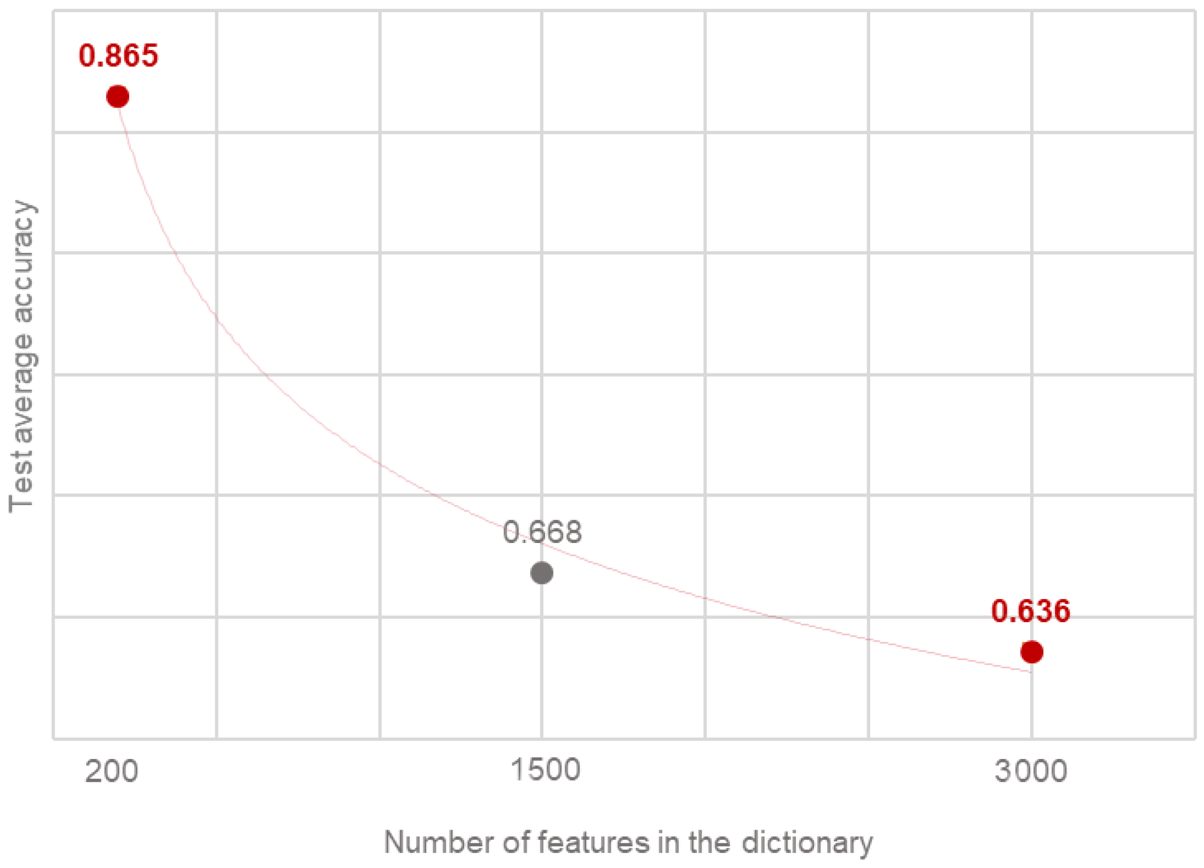
Figure 4 presents the accuracy of the average tests for each dictionary size. The higher the data dimensionality, the worse the k-NN’s accuracy. The difference between k-NN when dict = 200 and dict = 1500 or dict = 3000 is significant (≈$0.2$). To show the tendency, the power trend line was added to the graph. As we can see, the accuracy tends to change in a similar way. What is interesting, the power trend line and the exponential curve are alike. The only difference is that the arc of the first one is more symmetrical [47]. Hence, it may be concluded that in this case the accuracy experiences an exponential change.

The three k-NN models with the highest accuracy were chosen to be tested in Substage 3.

Table 14. Evaluation of the chosen classifiers performance in Substage 2.

k	Accuracy	Sensitivity	Specificity	PPV	NPV
11 (1)	0.915	0.938	0.892	0.897	0.935
9	0.912	0.923	0.900	0.902	0.921
11 (2)	0.908	0.915	0.900	0.902	0.914

presents the five indicator values. This allows performance of a more thorough evaluation.

Substage 3 consisted of ten tests. The first six of them were chosen as the top results of Substage 1 and Substage 2. The other four were conducted because of their promising performance in the previous experiments. The top accuracy values were obtained for the following parameters (these four models were designated for testing in Substages 4 and 5):

• MNB (1)—accuracy $=0.914$, dict = 3000, lemmatization;
• MNB (2)—accuracy $=0.909$, dict = 1500, lemmatization;
• NuSVC—accuracy $=0.885$, dict = 1500, stemming;
• k-NN $k=11$—accuracy $=0.828$, dict = 200, lemmatization.

Table 15. Evaluation of the chosen classifiers performance in Substage 3.

Model	Accuracy	Sensitivity	Specificity	PPV	NPV
MNB (1)	0.914	0.952	0.876	0.885	0.948
MNB (2)	0.909	0.950	0.868	0.878	0.945
NuSVC	0.885	0.805	0.965	0.959	0.832
k-NN $k=11$	0.828	0.719	0.938	0.920	0.769

includes the quality metrics related to the four models that will be tested in Substages 4 and 5. When compared to MNB, NuSVC and k-NN have lower accuracy, sensitivity, and NPV. However, both obtained better specificity and PPV parameters. On the other hand, MNB was better at predicting the negative class.

In Substage 4, once again, MNB models achieved the highest values of accuracy: $0.919$ and $0.909$. Surprisingly, k-NN with $k=11$ performed slightly better than NuSVC. Except for NuSVC, all models obtained higher accuracy than in Substage 3.

A collection of values that facilitate assessing the performance of the classifiers in Substage 4 is presented in

Table 16. Evaluation of the classifiers performance in Substage 4.

Model	Accuracy	Sensitivity	Specificity	PPV	NPV
MNB (1)	0.919	0.976	0.863	0.877	0.973
MNB (2)	0.909	0.972	0.846	0.863	0.968
NuSVC	0.829	0.996	0.662	0.746	0.995
k-NN $k=11$	0.860	0.865	0.855	0.856	0.863

. A very low specificity was noted for NuSVC. The model made a considerable mistake by classifying 933 ham e-mails as spam. The number was approximately two times higher than in the case of the other classifiers.

Substage 5 aimed at testing the classifiers that had performed best in Substage 3, but on the dataset that was not related to Enron. The sizes of dataset 1 and the one used in this substage (dataset 4, extracted from Lingspam corpus) were the same and that is why the accuracies will be compared to those obtained in Substage 1. The training set consisted of 702 e-mails. In the test set, there were 260 messages. In both cases, when MNB classified the messages, it achieved the highest accuracy. For MNB (1), there were 3000 features in the dictionary, for MNB (2)—1500. In each case, the lemmatization was added to the program. k-NN fared the worst—much less than it achieved in Substage 1, when its accuracy was $0.915$ for the same parameters. This may be a result of the source dataset content (Enron vs. Lingspam). NuSVC improved its accuracy by $0.157$.

Table 17. Evaluation of the classifiers performance in Substage 5.

Model	Accuracy	Sensitivity	Specificity	PPV	NPV
MNB (1)	0.962	0.923	1	1	0.929
MNB (2)	0.962	0.923	1	1	0.929
NuSVC	0.915	0.862	0.969	0.966	0.875
k-NN $k=11$	0.796	0.608	0.985	0.975	0.715
Results obtained by G. Piatetsky-Shapiro and M. Mayo [29]
MNB	0.962	0.931	0.992	0.992	0.935

summarizes metrics for the 4 models tested in Substage 5 and for the results obtained by G. Piatetsky-Shapiro and M. Mayo in a similar experiment on the same dataset [29]. The probability that k-NN classified a harmful message as spam is only $0.608$—this is the bottom value among all results. This fact has a direct impact on the accuracy of k-NNs, which was the lowest one in this substage. Both MNB models obtained specificity and PPV equal to 1. It means there was not a single non-spam e-mail that would be misclassified as spam. Moreover, the total number of misclassified e-mails was only 10 (spam classified as ham). In Substage 5, for dataset 4, MNB classifier turned out to be nearly perfect. The results are a little better than those achieved by G. Piatetsky-Shapiro and M. Mayo [29]. This is possibly because of the more complex text-preprocessing methods that were implemented.

4.4. Method Validation and Discussion of Results

First, we note that text preprocessing has a significant impact on the behavior of the classifiers. There is no doubt it is always beneficial to apply the basic methods, such as conversion to lowercase (or uppercase as the effect is the same), removing stop words, digits or punctuation marks and other techniques, as described in Figure 2. Implementing advanced text-preprocessing methods (stemming or lemmatization) allows the acquisition of higher accuracy of the classification.

Second, the selected size of the dictionary (the number of features) matters. For the support vector machines and naïve Bayes classification, the results were better if the number of features was larger. On the contrary, k-NNs’ accuracy tends to decrease rapidly for higher data dimensionality. k-NN obtained the highest accuracy for the smallest dictionary size. k-NN performs well when that data dimensionality is low. Its efficiency is also highly dependent on the k parameter. It might be assumed that if k-NN achieves the maximum accuracy for the given $k_{max}$, the performance will experience a sharp drop for $k>k_{max}$. Testing the support vector classification methods proved that LinearSVC is relatively efficient when the dataset is small. For large datasets NuSVC classification is more accurate.

Third, among all designed classifiers, MNB turned out to be a leader. In the relevant stages, the maximum accuracy across all results was obtained by MNB. Naïve Bayes classification is efficient in all cases but eventually returns the best outcomes when the dictionary consists of many features and the lemmatization technique is included in the application.

Fourth, the classifiers that achieved the best results when tested on the extract from the Enron Corpus, classified the e-mails even more accurately for the dataset extracted from the Lingspam corpus. This indicates that the content (words) and the structure of the data impact the model performance directly.

Fifth, the most important aspect related to validation of our work is related to the quality of the obtained results. Here, one of the most important aspect of our proposal is summarized with

Table 18. Comparison of the validation results with various performance metrics.

Method	Measure	Our Result	Results Reported in the Literature
MNB	Accuracy	0.962	0.477 [7], 0.598 [24], 0.832 [23], 0.898 [11], 0.917 [14], 0.957 [10], 0.962 [29], 0.994 [5]
MNB	Sensitivity	0.923	0.496 [7], 0.897 [11], 0.931 [29]
MNB	Specificity	1 .000	0.516 [7], 0.900 [11], 0.992 [29]
SVM	Accuracy	0.915	0.840 [24], 0.917 [14], 0.919 [11], 0.940 [12], 0.962 [5], 0.966 [22], 0.971 [10]
SVM	Sensitivity	0.867	0.901 [12], 0.918 [11], 0.976 [22]
SVM	Specificity	0.969	0.920 [11]
k-NN	Accuracy	0.796	0.453 [7], 0.846 [23], 0.908 [11], 0.920 [13], 0.990 [21]
k-NN	Sensitivity	0.608	0.319 [7], 0.921 [11]
k-NN	Specificity	0.985	0.478 [7], 0.887 [11]

. It shows a signification progress in comparison with the results reported in the referenced literature (the highest values are marked in red). One can see that especially the specificity provided by our approach is attractive. It is important in the case of unbalanced datasets and applications related to anomaly detection (where spam detection is also assigned).

5. Summary

The proposed multistage meta-algorithm for checking the classifiers performance, including an experimental method that involves the use of cross-validation between different datasets, allowed us to obtain reliable performance metrics in our illustrative example limited to the three important and representative classifiers. According to our results, which are consistent with other literature studies (but also typically outperform them from the viewpoint of the used metrics, especially aligned with unbalanced datasets), the multinomial naïve Bayes classifier is a method that once combined with well-thought text-preprocessing techniques as used in our meta-algorithm, may turn into the best weapon against spammers, who are becoming wiser every day. The advantage of our solution is that it can work with large datasets and give reliable results in a short time period by introducing the concept of fast recognition of the most interesting parameters. Moreover, the proposed method allows for cross-validation between different datasets in training and test phases.

Finally, the whole validation study presented in the paper based on our multistage meta-algorithm, including especially many (five) substages of cross-validation, shows that the whole method is robust. It is run on a standard desktop PC and operates within minutes to prove the results.

References

- Bauer, E. 15 Outrageous Email Spam Statistics that Still Ring True in 2018. Available online: https://www.propellercrm.com/blog/email-spam-statistics (accessed on 6 August 2021).
- Symantec. Internet Security Threat Report. 2019. Available online: https://www.symantec.com/content/dam/symantec/docs/reports/istr-24-2019-en.pdf (accessed on 6 August 2021).
- Ferrara, E. The History of Digital Spam. Commun. ACM 2019, 62, 82–91. [Google Scholar] [CrossRef] [Green Version]
- Dada, E.G.; Bassi, J.S.; Chiroma, H.; Adetunmbi, A.O.; Ajibuwa, O.E. Machine Learning for Email Spam Filtering: Review, Approaches and Open Research Problems. Heliyon 2019, 5, e01802. [Google Scholar] [CrossRef] [PubMed] [Green Version]
- Awad, W.A.; ELseuofi, S.M. Machine Learning Methods for Spam E-Mail Classification. Int. J. Comput. Sci. Inf. Technol. 2011, 3, 173–184. [Google Scholar] [CrossRef]
- Sharma, S.; Arora, A. Adaptive Approach for Spam Detection. Int. J. Comput. Sci. Issues 2013, 10, 23. [Google Scholar]
- Harisinghaney, A.; Dixit, A.; Gupta, S.; Arora, A. Text and Image Based Spam Email Classification using KNN, Naïve Bayes and Reverse DBSCAN Algorithm. In Proceedings of the International Conference on Reliability Optimization and Information Technology (ICROIT), Faridabad, India, 6–8 February 2014; pp. 153–155. [Google Scholar] [CrossRef]
- Sharma, D. Experimental Analysis of KNN with Naive Bayes, SVM and Naive Bayes Algorithms for Spam Mail Detection. Int. J. Comput. Sci. Technol. 2016, 7, 225–228. [Google Scholar]
- Sharma, U.; Khurana, S.S. SHED: Spam Ham Email Dataset. Int. J. Recent Innov. Trends Comput. Commun. 2017, 5, 1078–1082. [Google Scholar]
- Jawale, D.S.; Mahajan, A.G. Hybrid Spam Detection using Machine Learning. Int. J. Adv. Res. Ideas Innov. Technol. 2018, 4, 2828–2832. [Google Scholar]
- Bassiouni, M.; Ali, M.; El-Dahshan, E.A. Ham and Spam E-Mails Classification Using Machine Learning Techniques. J. Appl. Secur. Res. 2018, 13, 315–331. [Google Scholar] [CrossRef]
- Shajideen, N.M.; Bindu, V. Spam Filtering: A Comparison between Different Machine Learning Classifiers. In Proceedings of the Second International Conference on Electronics, Communication and Aerospace Technology (ICECA), Coimbatore, India, 29–31 March 2018; pp. 1919–1922. [Google Scholar] [CrossRef]
- Suryawanshi, S.; Goswami, A.; Patil, P. Email Spam Detection: An Empirical Comparative Study of Different ML and Ensemble Classifiers. In Proceedings of the IEEE 9th International Conference on Advanced Computing (IACC), Tiruchirappalli, India, 13–14 December 2019; pp. 69–74. [Google Scholar] [CrossRef]
- Shahariar, G.M.; Biswas, S.; Omar, F.; Shah, F.M.; Hassan, S.B. Spam Review Detection Using Deep Learning. In Proceedings of the IEEE 10th Annual Information Technology, Electronics and Mobile Communication Conference (IEMCON), Vancouver, BC, Canada, 17–19 October 2019; pp. 0027–0033. [Google Scholar] [CrossRef]
- Swetha, M.S.; Sarraf, G. Spam Email and Malware Elimination Employing Various Classification Techniques. In Proceedings of the 4th International Conference on Recent Trends on Electronics, Information, Communication and Technology (RTEICT), Bangalore, India, 17–18 May 2019; pp. 140–145. [Google Scholar] [CrossRef]
- Gaurav, D.; Tiwari, S.M.; Goyal, A.; Gandhi, N.; Abraham, A. Machine Intelligence-based Algorithms for Spam Filtering on Document Labeling. Soft Comput. 2020, 24, 9625–9638. [Google Scholar] [CrossRef]
- Ablel-Rheem, D.M.; Ibrahim, A.O.; Kasim, S.; Almazroi, A.A.; Ismail, M.A. Hybrid Feature Selection and Ensemble Learning Method for Spam Email Classification. Int. J. Adv. Trends Comput. Sci. Eng. 2020, 9, 217–223. [Google Scholar] [CrossRef]
- Kumar, N.; Sonowal, S. Nishant, Email Spam Detection Using Machine Learning Algorithms. In Proceedings of the Second International Conference on Inventive Research in Computing Applications (ICIRCA), Coimbatore, India, 15–17 July 2020; pp. 108–113. [Google Scholar] [CrossRef]
- Gibson, S.; Issac, B.; Zhang, L.; Jacob, S.M. Detecting Spam Email with Machine Learning Optimized with Bio-Inspired Metaheuristic Algorithms. IEEE Access 2020, 8, 187914–187932. [Google Scholar] [CrossRef]
- Karimovich, G.S.; Jaloldin ugli, K.S.; Salimbayevich, O.I. Analysis of Machine Learning Methods for Filtering Spam Messages in Email Services. In Proceedings of the International Conference on Information Science and Communications Technologies (ICISCT), Tashkent, Uzbekistan, 4–6 November 2020; pp. 1–4. [Google Scholar] [CrossRef]
- Nandhini, S.; Marseline, K.S. Performance Evaluation of Machine Learning Algorithms for Email Spam Detection. In Proceedings of the International Conference on Emerging Trends in Information Technology and Engineering (ic-ETITE), Vellore, India, 24–25 February 2020; pp. 1–4. [Google Scholar] [CrossRef]
- Saidani, N.; Adi, K.; Allili, M.S. A Semantic-Based Classification Approach for an Enhanced Spam Detection. Comput. Secur. 2020, 94, 101716. [Google Scholar] [CrossRef]
- Hossain, F.; Uddin, M.N.; Halder, R.K. Analysis of Optimized Machine Learning and Deep Learning Techniques for Spam Detection. In Proceedings of the IEEE International IOT, Electronics and Mechatronics Conference (IEMTRONICS), Toronto, ON, Canada, 21–24 April 2021; pp. 1–7. [Google Scholar] [CrossRef]
- Rastenis, J.; Ramanauskaitė, S.; Suzdalev, I.; Tunaitytė, K.; Janulevičius, J.; Čenys, A. Multi-Language Spam/Phishing Classification by Email Body Text: Toward Automated Security Incident Investigation. Electronics 2021, 10, 668. [Google Scholar] [CrossRef]
- Şahin, D.Ö.; Demirci, S. Spam Filtering with KNN: Investigation of the Effect of k Value on Classification Performance. In Proceedings of the 2020 28th Signal Processing and Communications Applications Conference (SIU), Gaziantep, Turkey, 5–7 October 2020; pp. 1–4. (In Turkish). [Google Scholar] [CrossRef]
- Maria; James, M.; Mruthula, M.; Bhaskaran, V.; Asha, S. Evasion Attacks On SVM Classifier. In Proceedings of the 2019 9th International Conference on Advances in Computing and Communication (ICACC), Kochi, India, 6–8 November 2019; pp. 125–129. [Google Scholar] [CrossRef]
- Di Mauro, M.; Longo, M. Skype Traffic Detection: A Decision Theory Based Tool. In Proceedings of the 2014 International Carnahan Conference on Security Technology (ICCST), Rome, Italy, 13–16 October 2014; pp. 1–6. [Google Scholar] [CrossRef]
- Di Mauro, M.; Longo, M. A Decision Theory Based Tool for Detection of Encrypted WebRTC Traffic. In Proceedings of the 2015 18th International Conference on Intelligence in Next Generation Networks, Paris, France, 17–19 February 2015; pp. 89–94. [Google Scholar] [CrossRef]
- Mayo, M.; Piatetsky-Shapiro, G. Email Spam Filtering: An Implementation with Python and Scikit-Learn. 2017. Available online: https://www.kdnuggets.com/2017/03/email-spam-filtering-an-implementation-with-python-and-scikit-learn.html (accessed on 6 August 2021).
- Radicati. Email Statistics Report, 2019–2023. Available online: https://www.radicati.com/wp/wp-content/uploads/2018/12/Email-Statistics-Report-2019-2023-Executive-Summary.pdf (accessed on 6 August 2021).
- SpamAssasin. Available online: https://spamassassin.apache.org/old/publiccorpus/ (accessed on 6 August 2021).
- SpamAssasin. Available online: https://spamassassin.apache.org (accessed on 6 August 2021).
- Project Honeypot. Available online: https://www.projecthoneypot.org (accessed on 6 August 2021).
- MailBait. Available online: https://mailbait.info (accessed on 6 August 2021).
- Enron Email Dataset; Athens University of Economics and Business. Available online: http://www2.aueb.gr/users/ion/data/enron-spam (accessed on 6 August 2021).
- Androutsopoulos, I.; Metsis, V.; Paliouras, G. Spam Filtering with Naive Bayes—Which Naive Bayes? In Proceedings of the CEAS Third Conference on Email and Anti-Spam 2006, CEAS 2006, Mountain View, CA, USA, 27–28 July 2006. [Google Scholar]
- Kadhim, A. An Evaluation of Preprocessing Techniques for Text Classification. Int. J. Comput. Sci. Inf. Secur. 2018, 16, 22–32. [Google Scholar]
- Wikipedia. Stop Words. Available online: https://en.wikipedia.org/wiki/Stopwords (accessed on 6 August 2021).
- Jabeen, H. Stemming and Lemmatization in Python. 2018. Available online: https://www.datacamp.com/community/tutorials/stemming-lemmatization-python (accessed on 6 August 2021).
- Trudgian, D. Spam Classification Using Nearest Neighbour Techniques. In Proceedings of the Intelligent Data Engineering and Automated Learning, IDEAL 2004, Exeter, UK, 25–27 August 2004; pp. 578–585. [Google Scholar] [CrossRef]
- Guttag, J.V. Introduction to Computation and Programming Using Python with Application to Understanding Data; The MIT Press: Cambridge, MA, USA, 2017. [Google Scholar]
- Stamp, M. Machine Learning with Applications in Information Security; CRC Press: Boca Raton, FL, USA, 2018. [Google Scholar]
- Hackeling, G. Mastering Machine Learning with Scikit Learn, 2nd ed.; Packt Publishing: Birmingham, UK, 2017. [Google Scholar]
- Christmann, A.; Steinwart, I. Support Vector Machines; Springer: New York, NY, USA, 2008. [Google Scholar]
- Stamp, M. A Survey of Machine Learning Algorithms and Their Application in Information Security. In Computer Communications and Networks—Guide to Vulnerability Analysis for Computer Networks and Systems; Springer: Cham, Switzerland, 2018; pp. 33–55. [Google Scholar] [CrossRef]
- Scikit-learn. Multinomial Naive Bayes. Available online: https://scikitlearn.org/stable/modules/naivebayes:htm (accessed on 6 August 2021).
- Excel Trendline Types, Equations and Formulas. Available online: https://www.ablebits.com/office-addins-blog/2019/01/16/excel-trendline-types-equations-formulas (accessed on 6 August 2021).
Figure 1.
The proposed multistage meta-algorithm for performance check of the spam detection algorithms.
Figure 2.
Text preprocessing steps.
Figure 3.
k-NN accuracy vs. k.
Figure 4.
Accuracy of the average tests vs. dictionary length.