Open Circuit Fault Diagnosis and Fault Tolerance of Three-Phase Bridgeless Rectifier

School of Mechanical Electronic & Information Engineering, China University of Mining and Technology Beijing, Ding No. 11 Xueyuan Road, Haidian District, Beijing 100083, China
*
Author to whom correspondence should be addressed.
Electronics 2018, 7(11), 291; https://doi.org/10.3390/electronics7110291
Submission received: 5 October 2018
/
Revised: 30 October 2018
/
Accepted: 30 October 2018
/
Published: 1 November 2018
(This article belongs to the Special Issue Applications of Power Electronics)
Abstract
:Bridgeless rectifiers are widely used in many applications due to a unity power factor, lower conduction loss and high efficiency, which does not need bidirectional energy transmission. In this case, the potential failures are threatening the reliability of these converters in critical applications such as power supply and electric motor driver. In this paper, open circuit fault is analyzed, taking a three-phase bridgeless as an example. Interference on both the input and output side are considered. Then, the fault diagnosis method including detection and location, and fault tolerance through additional switches are proposed. At last, simulation and experiments based on the hardware in loop technology are used to validate the feasibility of fault diagnosis and fault tolerance methodology.
1. Introduction
Multilevel converters have been widely used in middle- and high-voltage application fields in the past decades, such as renewable energy, adjustable speed drive, power transmission network, electric vehicle [1] etc. Topologies of these converters including H Bridge-based, neutral point clamping-based and bridgeless-based are most popular in literatures. Recently, bridgeless-based topologies have drawn increasing attention from industry and academia due to its high efficiency, low loss and simplification control strategy [2,3,4,5,6]. Compared with H Bridge-based converters, these bridgeless-based converters cannot work as inverters. However, considering that the applications are mostly pumps, fans and compressors which only need the power flowing unidirectionally [7], H-bridge-based converter has gradually been substituted by bridgeless-based converters as a pulse width modulation (PWM) rectifier in these fields. The bridgeless-based converter as a rectifier provides a sinusoidal input current at unity power factor and a controllable dc output voltage.
With the growing power switch numbers and power density, reliability of power electronic converters is increasingly important because the malfunctions are unacceptable and cause serious losses (e.g., nonscheduled downtime) in the critical applications. As a kind of electric energy conversion device, three-phase bridgeless converter (3-BLC) also endures high frequency voltage shock, over temperature impact, overload and improper driving signal. Semi-conductor devices, especially power switches, will fail more easily than other components. As discussed in Reference [8], the power switches contribute to 31% of failures, which are the most fragile components among capacitors, gate drivers, resistors and inductors. Power switches faults are usually caused by bond-wire lift-off or solder cracking, which will lead to an open circuit or short circuit of converters. The faults are named open circuit faults (OCF) and short circuit faults (SCF) respectively. An SCF will cause a large current and result in system shutdown, so hardware-based approaches such as fast fuses or breakers to transfer an SCF to an OCF are generally used. An OCF will not shutdown a system immediately but it degrades the performance inconspicuously. These may, in turn, cause secondary faults. Therefore, it is necessary to study a fault diagnosis and tolerance method for power switches OCF of the rectifier in this article.
In the past decade, numerous fault diagnosis and tolerance methods have been proposed for power electronic converters in the literature [9,10,11,12,13,14,15,16]. However, there are a few research works for ac-dc rectifiers, especially bridgeless rectifiers. For example, a diagnosis method based on a mixed logical dynamic model and residual generation was applied to a single-phase rectifier in a railway electrical traction drive system [17]. This method was fast, simple and stable, but it does not suit three-phase systems. For three-phase conditions, a current waveforms-based similarity analysis method for a three-phase PWM rectifier was proposed in Reference [18]; current waveforms were analyzed pairwise to diagnose an open circuit fault. There was a critical drawback of this method that it ignored the three-phase voltage imbalance, which is often seen for grid. In Reference [19], a fault tolerance control with additional devices for three-phase soft-switching mode rectifier is proposed. The circuit configuration had two extra center-tapped autotransformers and three more toggle switches compared with the traditional system. This method was more suitable for new design, but more retrofit cost was demanded for the existing systems. Considering the dc voltage decrease by OCF, Reference [20] proposed a fault tolerant method for the three-level rectifier in a wind turbine system, which was implemented by adding a compensation value to the reference voltages. The proposed method preserved the power factor under faulty conditions utilizing the redundancy of the switching devices, where the 3-BLC does not have such ability.
This study aims for an OCF diagnosis and tolerance method for bridgeless-based rectifiers [21,22,23], especially the 3-BLC. The contribution of this paper is to propose a fault feature extraction method for 3-BLC, and a fault tolerant method based on an extra two switches. The fault features were extracted from the three-phase currents. Load sudden change, source voltage imbalance or fluctuation and harmonic interference have been considered to prevent the impact on the proposed method. After that, the OCF is identified by a mixed logical model-based algorithm. When a fault was diagnosed, the drive signals of the faulty phase were redistributed artificially by the additional switches. Thus, it will maintain the current path in failure condition and make the 3-BLC still work as normal.
The rest of this paper is organized as follows. In Section 2, the mathematical model of single and three-phase bridgeless converters are analyzed. In Section 3, the fault diagnosis with an improvable feature extraction method is proposed. Section 4 details the fault tolerant implementation through additional devices. System validation using simulation and experiment data is provided in Section 5. Finally, conclusions are drawn in Section 6.
2. Basic Principles of Three-Phase Bridgeless Converters
2.1. Structure and Operation of 3-BLC
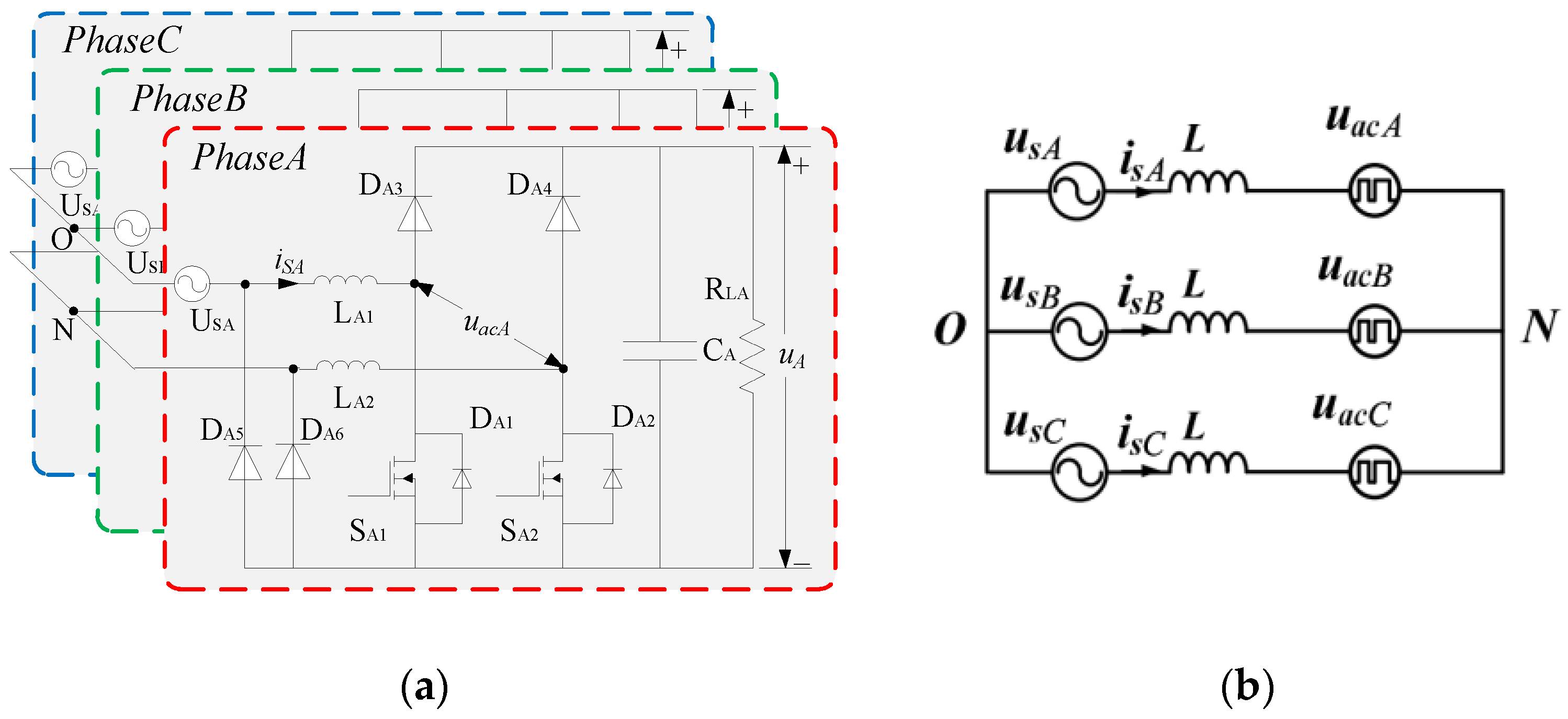
A three-phase bridgeless converter (3-BLC) is shown in Figure 1a. As can be seen, this three-phase converter is expanded from a single-phase dual-boost bridgeless structure, which has additional slow-recovery diodes D5 & D6 and two boost inductors L1 & L2 to reduce common mode noise [24,25]. Compared to the H bridge structure, bridgeless structure reduces 50% of fully controlled switches. Therefore, the control circuits, gate drivers, as well as protection units are greatly reduced, thus decreasing the system complexity and switching losses drastically [26]. The equivalent ac side circuit is depicted in Figure 1b and the mathematical model of 3-BLC can be expressed as
where are the ac voltages of phase A, B and C; is the neutral point voltage; is the inductance of L1 and L2.
In order to clarify the analysis process, in this study, the slow-recovery diodes are temporarily substituted by the body diodes and the boost inductors are equivalent to an inductor L. Therefore, taking a single-phase bridgeless rectifier as an example, Figure 2 shows its principles on four operating modes. In this study, the power switches S1 and S2 are synchronously turned ON and OFF, which is named synchronous control scheme. Define as a switch function of this converter. When , S1 and S2 are both turned ON, the power is transferred to power storage inductor L as shown in Figure 2a,c. When , S1 and S2 are both turned OFF, the power stored in inductor L is transferred to the load side as shown in Figure 2b,d. Then, a bulky electrolytic capacitor C is employed to buffer the power and, hence, smooth the output voltage. Thus, the steady-state mathematic model can be yielded by applying KVL and KCL as following.
where is the inductance of the power storage inductor, is the capacitance of the output capacitor, is the resistance of load, is the input current, is the capacitor voltage, is the ac voltage, and .
Applying the volt-second balance and ampere-second balance principles to Equation (2) derives
where is the duty cycle.
2.2. Open Circuit Fault Analysis
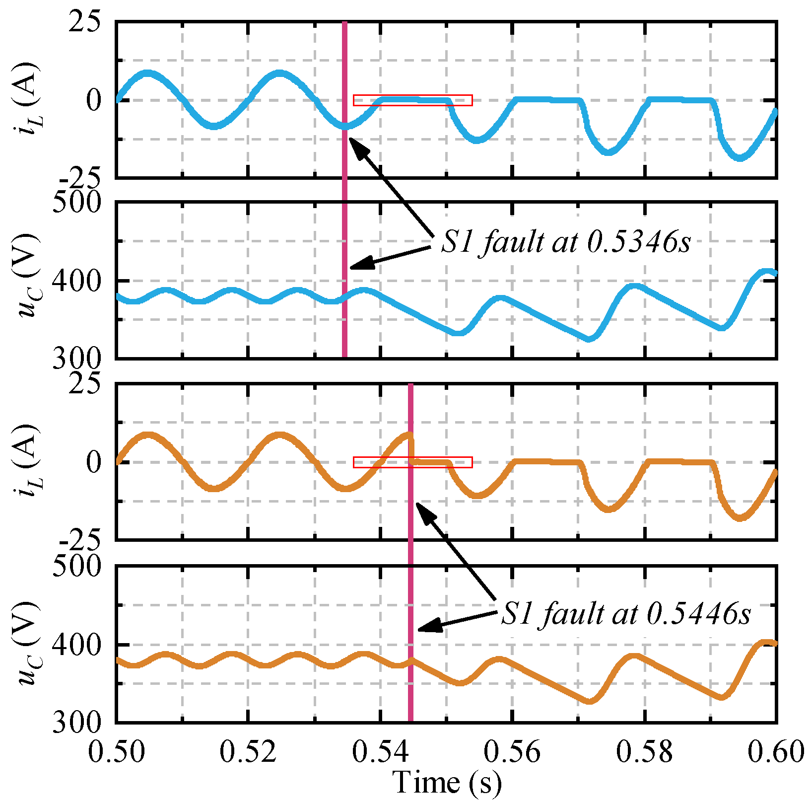
As described above, there are four operating modes which generate through the ac voltage polarity and the switching states. When a switch fails due to physical damage or improperly driving signal, the corresponding operating mode no longer exists. This will cause changes on the related signals, which is called fault features, and is the theoretical foundation of fault detection and location. In the rest of this section, fault features of S1 OCF were analyzed as an example. Because power switches are the most fragile component and an SCF can be converted to an OCF by fast fuses immediately, the current and voltage waveforms shown in this section were acquired by simulations. The fault times were set in the positive and negative ac cycle of the input voltage respectively.
When an OCF occurs on switch S1, the power storage path as shown in Figure 2a is disconnected. Therefore, the converter works only in power discharging mode as shown in Figure 2b. However, in the negative ac cycle, the converter works properly because S1 is not in both a power charging and discharging path. The waveform of the input current and capacitor voltage during S1 open circuit fault at different half cycles are shown in Figure 3. Because it is a non-resonant circuit, the large impedance makes the input current fell into nearly zero after S1 failed in negative ac cycle, but it seems normal in positive ac cycles. The capacitor voltage resembles the input current which double frequency ripple disappears obviously after 0.5446 s, but it seems no change after 0.5346s until a positive ac cycle. The features of input current and capacitor voltage before and after switch S2 fails are just like S1.
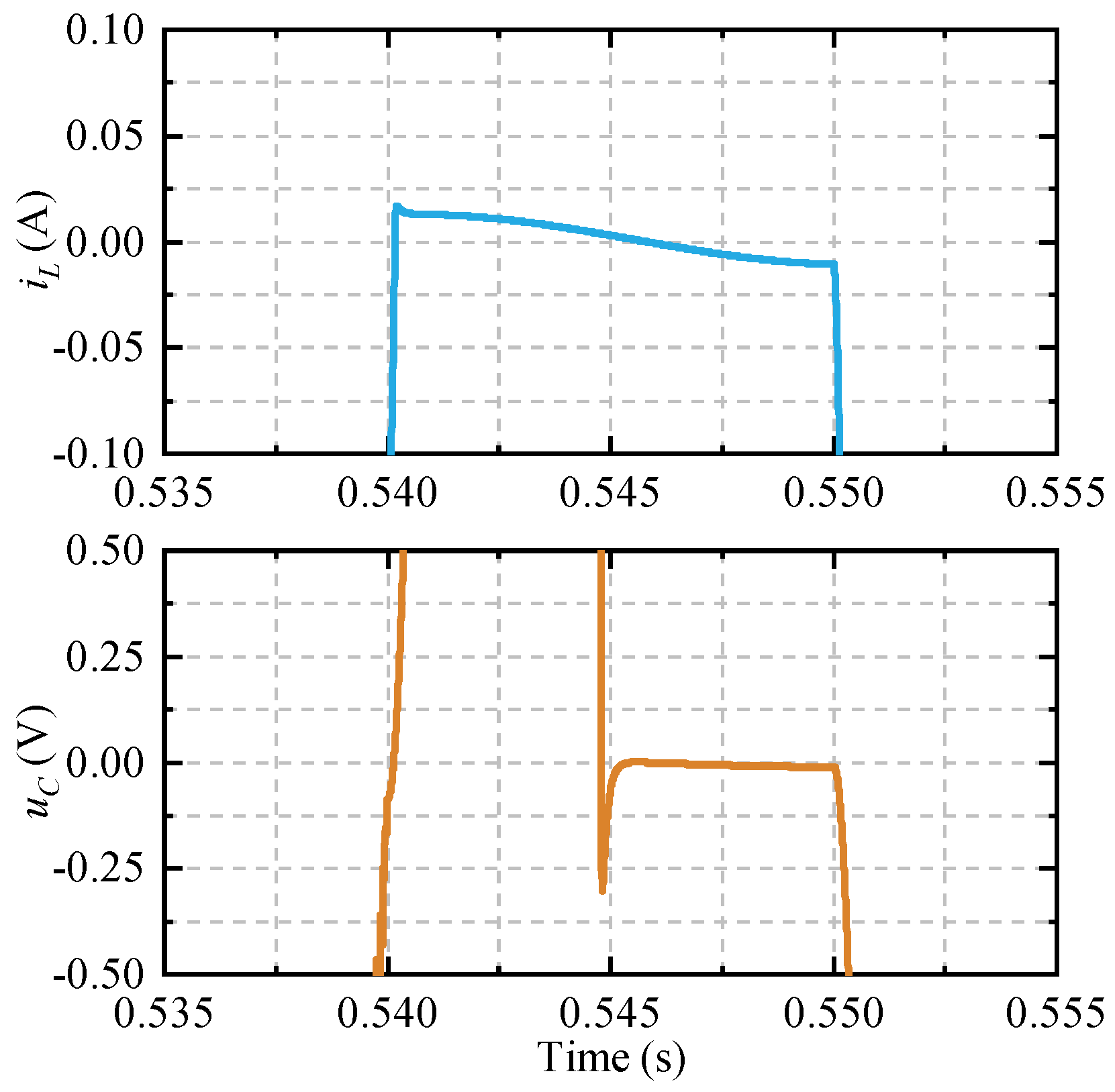
The dynamic details of the input current inside the red frame of Figure 3 are also shown in Figure 4. According to Equation (3), the duty cycle of one switch will mutate to zero when it occurred an OCF. Since the switching period no longer existed, the assumption that the input voltage is constant during the switching cycle was no longer valid. Due to the impedance of the inductor to the low frequency signal, the input current became zero after the energy in the inductor was released. The load voltage was maintained by the DC capacitor until another ac cycle which was not affected by the fault.
2.3. Input Side Interferences
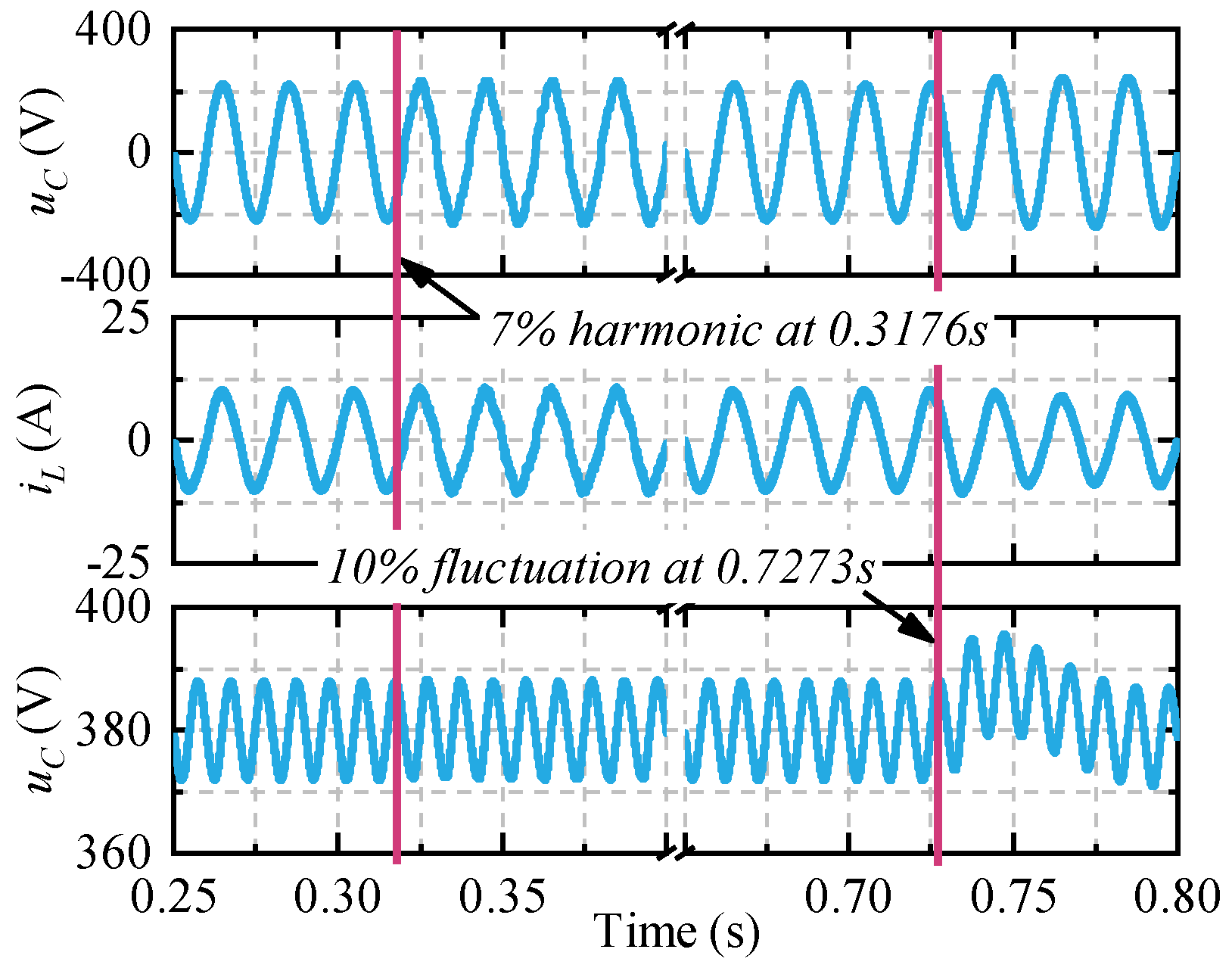
Voltage fluctuations and harmonic pollution are unavoidable on the input side. They will affect the characteristics of current and voltage signals which have an impact on the diagnosis of the fault. Thus, this study discusses the features of input current and capacitor voltage under input voltage fluctuation and harmonic pollution, which are shown in Figure 5. About 7% harmonic was injected to input voltage at 0.3176 s, consequently, the THD of the input current increased from 4% to 8% but the impact on the capacitor voltage was limited. Still, from this figure, the input voltage fluctuated about 10% higher at 0.7273 s. The input current decreased a little and the capacitor voltage jittered rapidly at the same time. Different from the failure conditions, these varieties recovered in a short time. The features are significantly different from those failures discussed in the previous paragraphs.
2.4. Load Side Interferences7
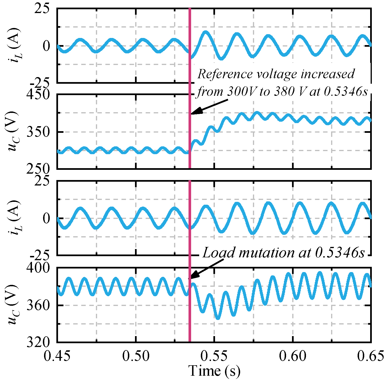
During the operation of the converters, the power on the load side was not always constant. The load sudden changed sometimes and the reference dc voltage also changed when transmitting different powers on the three-phase imbalance condition. This will lead to failure of fault diagnosis. In this study, output power variations due to reference voltage changed and load sudden change were also involved.
As shown in Figure 6, the reference output voltage increased from 300 V to 380 V at 0.5346 s, then the magnitude of the input current and capacitor voltage rose rapidly and became stable in two ac cycles. The output power saw a 60% growth from 400 W to 640 W. Still, in this figure, the load became heavier abruptly at the same time, which resulted in output power rising up to 1000 W with a 56% increment. The input current increased smoothly and rapidly, meanwhile the capacitor voltage decreased a little but restored fast with a higher ripple.
In summary, an OCF will result in input current falling to about zero and increasing ripple of the capacitor voltage. The intensity of current oscillation depended on the values of and . The features of input or load side interferences were essentially similar, and did not affect the sinusoidal characteristic of the input current and capacitor voltage signals. It has to be noticed that in these analyses, when switch S1 failed in a negative ac cycle, the converter maintained regular operation until a positive ac cycle, and vice versa for switch S2. The duration of this condition lasted up to a half ac cycle, which is related to the time of failures.
3. Fault Diagnosis Technique
Fault diagnosis is the basis of fault tolerant control and consisted of fault detection and fault location [27]. It is important to detect and locate a malfunction switch rapidly, taking into account the fault features. In addition, the performance within fault tolerant behavior, such as redundancy control, is not only affected by fault diagnosing time directly, but also fault diagnosing accuracy including misdiagnosis and missed diagnosis [28]. Therefore, the fault diagnosis algorithm needs to be simple and effective.
3.1. Fault Features Extraction
As aforementioned, the sinusoidal characteristic of input current is damaged when an OCF occurs, but is reserved under other interferences. Therefore, it is feasible to select the input current as the characteristic signal of fault diagnosis. Generally, it is straightforward to utilize frequency domain characteristics as fault features [29]. However, most of the frequency domain methods require Fast Fourier Transform (FFT), which costs large amounts of computation. In order to improve the diagnostic efficiency and reduce the computational cost, this study used a direct time domain analysis method. Considering a three-phase converter, an transformation, named Concordia transformation, is applied to analyze conveniently in a two-phase stationary coordinate system. This transformation can be expressed as
Transformed input current signals are shown in Figure 7, which took as the abscissa and as the ordinate. The gradient of color represented the increase of time; therefore, the characteristics of and before and after failure were revealed in these figures. Single switch failures of each switch were shown in Figure 7, as well as normal and load side interference conditions. Input side interference was similar with the load side.
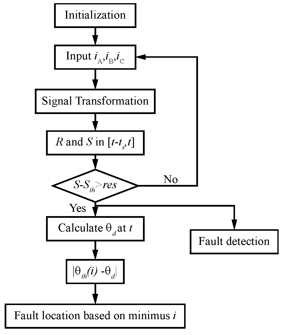
3.2. Fault Detection and Location Method
According to the features shown in the above figure, and constitute a circular trajectory under normal and interference conditions. However, an OCF will change the trajectory and different fault location will result in different trajectories. In other words, vectors from to contain distinguished features of OCFs. Define as the length of this vector, an interval increment-based fault detection method was proposed and can be expressed as
where is the accumulative bias of , is a reference value for detecting an OCF, is the threshold of residual for decision, and is the length of the interval. is the reference of which lags one ac cycle to increase the sensitivity, and is the power frequency cycle.
Review the angle between this vector and the positive direction of the abscissa axis. It can be found that the abnormal occurred at a specific angular interval corresponding to different fault locations. The central values of these intervals, defined as , are ideally taken as corresponding to SA1, SA2, SB1, SB2, SC1, SC2 OCFs one by one. Then, a fault location method after fault detection was proposed based on this vector. It selected the minus central value between the angle when a fault was detected and as the location judgment, which can be expressed as
where , which represents SA1, SA2, SB1, SB2, SC1, and SC2 respectively. is the angle when an OCF was detected.
The flow chart including fault detection and fault location algorithm are shown in Figure 8.
4. Fault Tolerance Method
An OCF will not cause the converter to shutdown immediately, but it slowly degrades the performance and reliability. Actually, a converter is desired to have the capability to operate in a quasi-normal condition in the post-failure period. Therefore, a fault tolerance method includes two aspects: fault tolerant topology with an extra two switches and a corresponding fault tolerant control method were proposed.
Also in the case of a single phase, the converter consists of two fast recovery diodes and two power switches with body diodes [25]. A current loop is broken due to an open circuit fault. Therefore, in order to obtain fault tolerant capability, additional devices must be added to restore the original current loop in the fault state. A fault tolerant topology with an additional two power switch which connected in parallel across the two fast recovery diodes is shown in Figure 9a. As aforementioned, more than two-thirds of ac-dc rectifiers in motor drives of industry only require a single direction for energy transmission. Therefore, considering the efficiency, loss, and control algorithms, this topology still operates as a bridgeless converter in the normal state, although it is similar to the H-bridge structure. The fault tolerant control diagram with drive signal distribution is shown in Figure 9b.
The control method diagram includes two control loops: an inner current loop and an outer voltage loop. The role of the inner loop is to realize a unity power factor, and the role of the outer loop is to provide a controllable output DC voltage. The voltage controller and current controller are obtained as
The output of the double PI loop was compared with the carrier. Hence, in turn, the PWM signal was generated for signal distribution. At the same time, constant zero which means low level driving signal, was also generated.
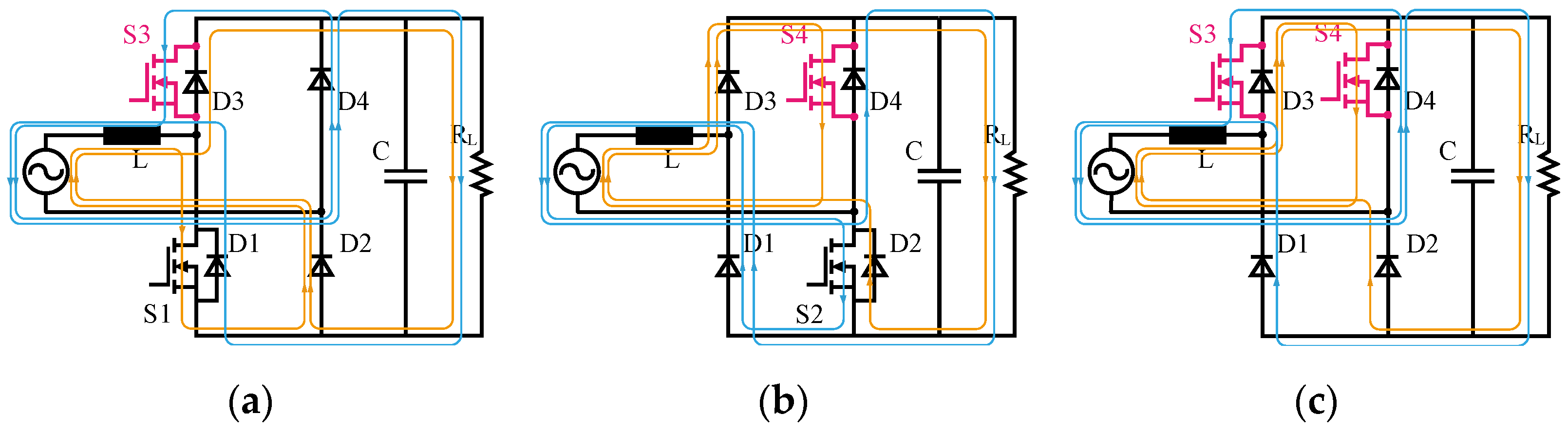
The converter achieved fault tolerance through dynamic structure reconfiguration [30,31]. According to the location of the faulty device, there are three substructure types after an OCF. Each of them has a corresponding drive signal distribution rule to maintain the normal operation of the converter. The circuit reconfigurations are shown in Figure 10.
In normal operation, both S3 and S4 are driven off by the low level, and S1 and S2 are driven by the PWM signal in a synchronous drive mode. When it is detected that an open circuit fault occurs in S2, S3 will be driven by which means S1 and S3 are driven by complementary signals. At this point, the circuit topology is converted into a totem pole bridgeless structure, as shown in Figure 10a. When an open circuit fault occurs in S1, the drive signal of S4 will also be replaced by , and S2 and S4 will continue to operate in a complementary signal drive mode. At this point, the circuit topology is converted to a symmetry totem pole bridgeless structure, as shown in Figure 10b. If an open circuit fault occurs in both S1 and S2, the circuit will be converted into a symmetry boost bridgeless structure consisting of S3 and S4, which will be driven by synchronously. This situation is shown in Figure 10c. The current path for the different topologies is also shown in Figure 10, with orange representing the path for the positive ac cycle and blue for the negative. The drive signal distribution table corresponding to each fault state is shown in Table 1.
5. Simulation and Experiment Results
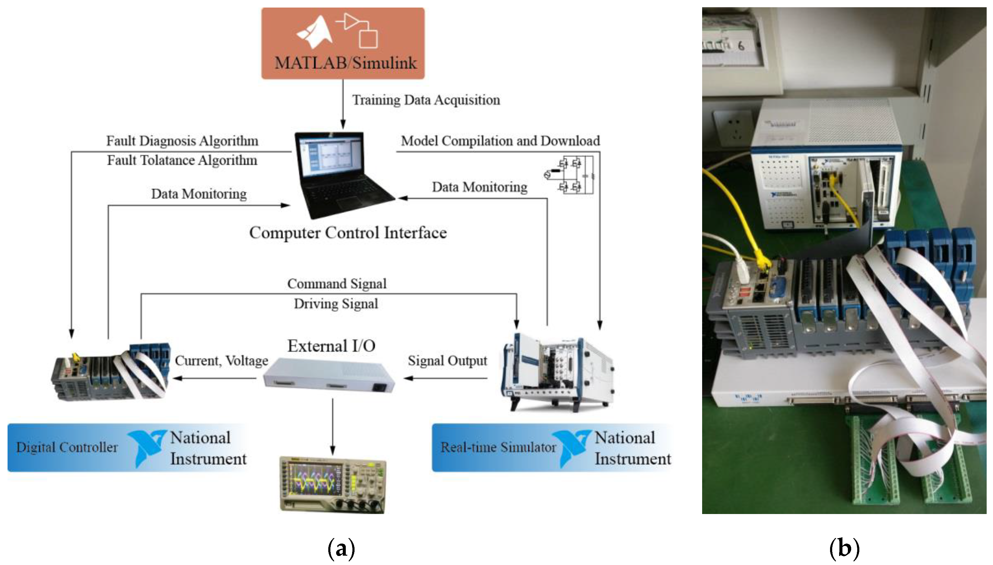
It is essential to demonstrate the proposed fault diagnosis and tolerant control method function as expected in a real converter. However, failures of a real device will lead to uncontrollable consequences such as burning or explosion. Therefore, hardware in loop (HIL) simulation technology is suitable for device failure experiments. In this study, simulation and experiment-based MATLAB/Simulink and NI platform were realized, as can be seen in Figure 11a; and the details concerning the equipment used in this setup are shown in Figure 11b.
The simulation model of the three-phase bridgeless converter was built in MATLAB/Simulink and used to verify the proposed fault diagnosis and tolerant control method. Then HIL simulation based on NI-PXI platform was employed to emulate physical experiment, which is widely recognized and adopted in the field of power electronic device failure researches [32]. The power system model was set up as shown in Figure 1, and the parameters are presented in Table 2. The simulation and experiment results are revealed in two aspects: fault diagnosis results and fault tolerant control results. It is noticed that there was no real fault and all the OCFs were emulated by focusing the low level drive signal of specific switches.
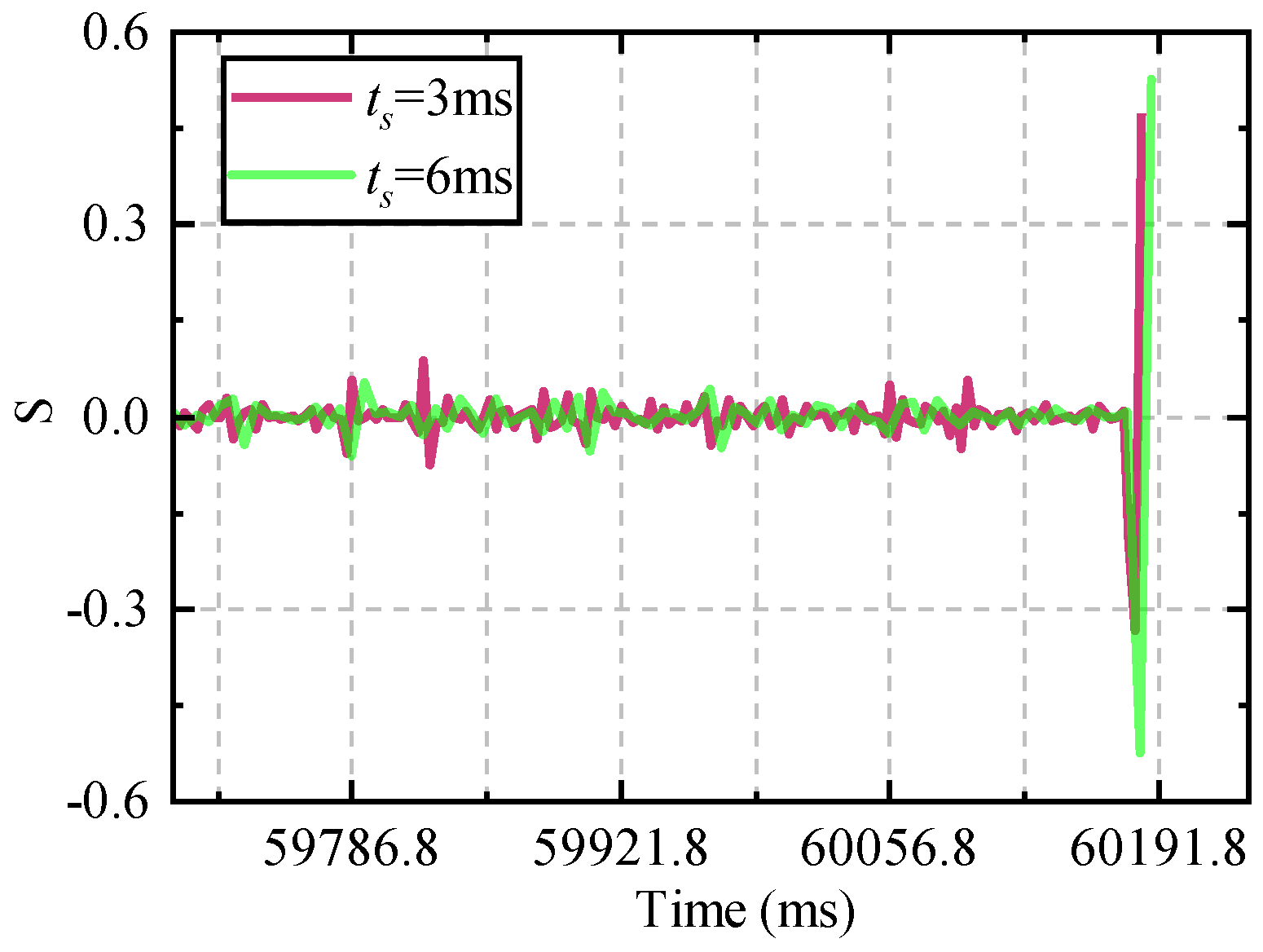
For the diagnostic algorithm proposed in this paper, the selection of has a direct impact on diagnostic resolution and diagnostic performance. Figure 12 shows the value of when is equal to 3 ms and 6 ms, plotted in red and green, respectively. Obviously, the diagnostic frequency (or resolution) of the proposed online real-time fault diagnosis is positively correlated with . In the normal state, the value of was about zero. When a fault occurred, began to fluctuate greatly. The amplitude was also positively correlated with . That is to say, a larger meaning larger diagnostic interval or lower diagnostic frequency can make it easier to identify a fault trigger, reduce misdiagnosis or missed diagnosis.
In order to make the method proposed in this study applicable with different system parameters, both and were normalized in the actual process. Furthermore, Figure 13 shows the results of 200 samples with different from 2 to 6 ms, where the average detection time is connected in green and the average accuracy rates in red. In this figure, the influence of different are also shown, in which the solid line represents and the dashed dotted line represents . When , as can be seen, the fault detection time increased as grew because it slowed down the diagnostic frequency, and the accuracy rates were maintained at around 98%. When , the detection time generally increased by about 20 ms, but there was greater decline in accuracy rates with growing. The reason is that longer integration time makes the value of closer to zero, and the larger threshold is gradually more unsuitable, resulting in a drop in the accuracy rate.
After selecting the appropriate parameters, the current signal and corresponding trigger signals collected by the oscilloscope were as shown in Figure 14.
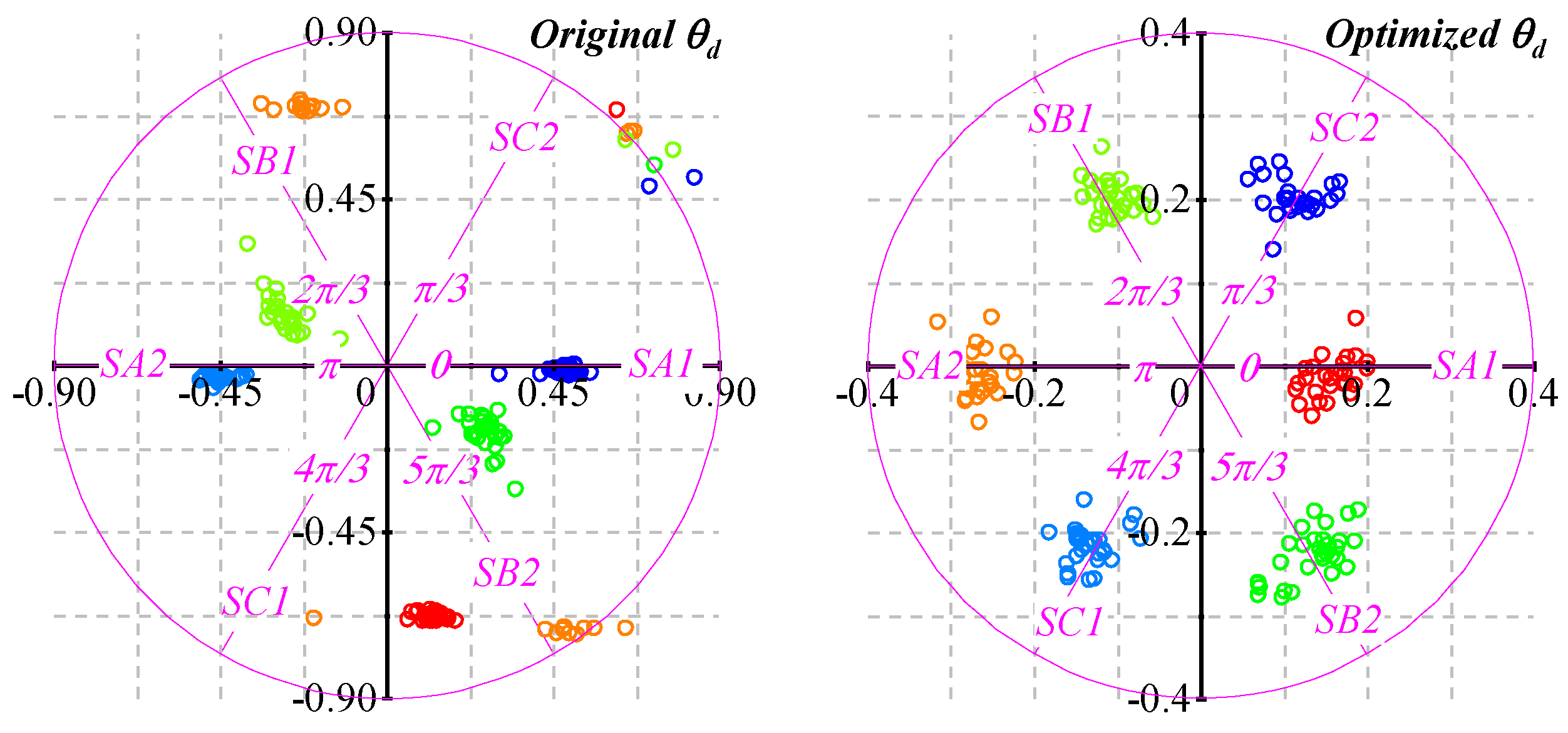
After a fault was detected, the fault location algorithm needed to be employed to locate the fault. Since the detected time was not the actual time at which a failure occurred. The calculated using and was disorderly, and therefore, it was impossible to locate the failure in practice. In this study, this problem was solved by sacrificing a certain fault tolerant time that the value of was taking as the time minimizing within a power cycle after . It can be expressed as
Figure 15 shows the scatter plots of and for each of the 30 samples. The pink auxiliary line identifies the angles corresponding to each fault under ideal conditions. The data points generated by original were scattered and could not be used for fault location. The optimized data points were concentrated in the vicinity of the ideal values which could be used for accurate fault location.
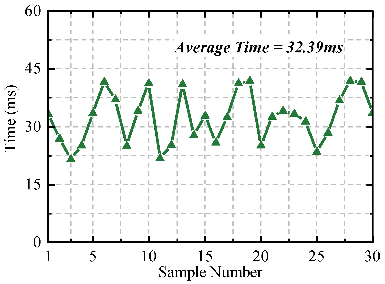
Under the condition of , 30 fault tolerance experiments were implemented where the faulty switch was randomly selected. The times from fault occurrence to fault tolerant control execution are shown in Figure 16. It can be found that the fault tolerance time increased by 20 ms relative to the detection time from Figure 13, where the delay of one ac cycle is caused by Equation (8).
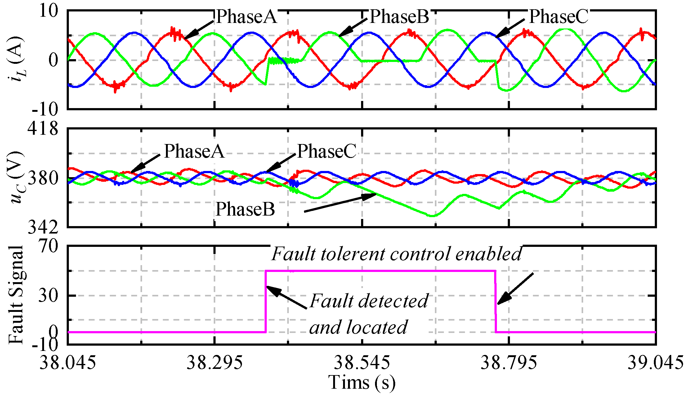
An example of fault diagnosis and tolerant control is shown in Figure 17. The signals were monitored by the host computer of the system built in this study.
In summary, the proposed fault diagnosis and fault tolerant control method were verified in simulation and experimentation. An OCF will be detected within at least 20 ms in general conditions, and tolerated with a 20 ms delay. Various interferences have limited impact on this algorithm. The accuracy of fault diagnosis was over 98%, and the error rate of the fault location and fault tolerance was zero.
6. Conclusions
Reliability is one of the primary concerns for the three-phase bridgeless converter. This paper presented an open circuit fault diagnosis and tolerant control method to maintain the converter running. As the basis for fault tolerance, the open circuit fault is detected and located accurately within a few milliseconds, thus, the abnormal operation time is reduced. Only two additional switches are needed to maintain the normal operation by structure reconfiguration. A lookup table is built for switch drive signals reconfiguration. Finally, the feasibility and effect of the proposed method on reliability promotion was verified by simulations and experiments. Furthermore, the interference analysis in this paper is still insufficient that the proposed method is not robust enough in practice. This requires further work.
Author Contributions
W.C., H.C. and C.W. conceptualized the main idea of this project; W.C. proposed the methods and designed the work; W.C. conducted the experiments and analyzed the data; J.D. checked the results; W.C. wrote the whole paper; and H.C., C.W., and J.D. reviewed and edited the paper.
Funding
This research was funded by National Natural Science Foundation of China under Grant 51577187.
Conflicts of Interest
The authors declare no conflict of interest.
References
- Blahnik, V.; Kosan, T.; Peroutka, Z.; Talla, J. Control of a Single-Phase Cascaded H-Bridge Active Rectifier under Unbalanced Load. IEEE Trans. Power Electron. 2018, 33, 5519–5527. [Google Scholar]
- Wang, C.; Zhuang, Y.; Jiao, J.; Zhang, H.; Wang, C.; Cheng, H. Topologies and Control Strategies of Cascaded Bridgeless Multilevel Rectifiers. IEEE J. Emerg. Sel. Top. Power Electron. 2017, 5, 432–444. [Google Scholar] [CrossRef]
- Kremes, W.D.J.; Font, C.H.I. Proposal of a three-phase bridgeless PFC SEPIC rectifier with MPPT for small wind energy systems. In Proceedings of the IEEE International Conference on Industry Applications, Curitiba, Brazil, 20–23 November 2016; pp. 1–8. [Google Scholar]
- Silva, C.E.A.; Oliveira, D.S.; Barreto, L.H.S.C.; Bascopé, R.P.T. A novel three-phase rectifier with high power factor for wind energy conversion systems. In Proceedings of the Power Electronics Conference (COBEP ’09), Bonito-Mato Grosso do Sul, Brazil, 27 September–1 October 2009; pp. 985–992. [Google Scholar]
- Park, S.M.; Park, S. Versatile Control of Unidirectional AC–DC Boost Converters for Power Quality Mitigation. IEEE Trans. Power Electron. 2015, 30, 4738–4749. [Google Scholar] [CrossRef]
- Whitaker, B.; Barkley, A.; Cole, Z.; Passmore, B.; Martin, D.; McNutt, T.R.; Lostetter, A.B.; Lee, J.S.; Shiozaki, K. A High-Density, High-Efficiency, Isolated On-Board Vehicle Battery Charger Utilizing Silicon Carbide Power Devices. IEEE Trans. Power Electron. 2014, 29, 2606–2617. [Google Scholar] [CrossRef]
- Malinowski, M.; Gopakumar, K.; Rodriguez, J.; Pérez, M.A. A Survey on Cascaded Multilevel Inverters. IEEE Trans. Ind. Electron. 2010, 57, 2197–2206. [Google Scholar] [CrossRef]
- Yang, S.; Bryant, A.; Mawby, P.; Xiang, D. An Industry-Based Survey of Reliability in Power Electronic Converters. IEEE Trans. Ind. Appl. 2011, 47, 1441–1451. [Google Scholar] [CrossRef]
- Yu, Y.; Zhao, Y.; Wang, B.; Huang, X.; Xu, D. Current sensor fault diagnosis and tolerant control for VSI-based induction motor drives. IEEE Trans. Power Electron. 2018, 33, 4238–4248. [Google Scholar] [CrossRef]
- Choi, U.; Lee, J.S.; Blaabjerg, F.; Lee, K.B. Open-Circuit Fault Diagnosis and Fault-Tolerant Control for a Grid-Connected NPC Inverter. IEEE Trans. Power Electron. 2016, 31, 7234–7247. [Google Scholar] [CrossRef]
- Wang, T.; Xu, H.; Han, J.; Bouchikhi, E. Cascaded H-Bridge Multilevel Inverter System Fault Diagnosis Using a PCA and Multi-class Relevance Vector Machine Approach. IEEE Trans. Power Electron. 2015, 30, 7006–7018. [Google Scholar] [CrossRef]
- Freire, N.; Estima, J.O.; Cardoso, A. A Voltage-Based Approach without Extra Hardware for Open-Circuit Fault Diagnosis in Closed-Loop PWM AC Regenerative Drives. IEEE Trans. Ind. Electron. 2014, 61, 4960–4970. [Google Scholar] [CrossRef]
- Freire, N.; Estima, J.O.; Cardoso, A. Open-Circuit Fault Diagnosis in PMSG Drives for Wind Turbine Applications. IEEE Trans. Ind. Electron. 2013, 60, 3957–3967. [Google Scholar] [CrossRef]
- Estima, J.O.; Cardoso, A.J.M. A New Approach for Real-Time Multiple Open-Circuit Fault Diagnosis in Voltage-Source Inverters. IEEE Trans. Ind. Appl. 2011, 47, 2487–2494. [Google Scholar] [CrossRef]
- Zidani, F.; Diallo, D.; Benbouzid, M.E.H.; Nait-Said, R. A fuzzy-based approach for the diagnosis of fault modes in a voltage-fed PWM inverter induction motor drive. IEEE Trans. Ind. Electron. 2008, 55, 586–593. [Google Scholar] [CrossRef] [Green Version]
- Aly, M.; Ahmed, E.; Shoyama, M. A New Single Phase Five-Level Inverter Topology for Single and Multiple Switches Fault Tolerance. IEEE Trans. Power Electron. 2018, 33, 9198–9208. [Google Scholar] [CrossRef]
- Gou, B.; Ge, X.; Wang, S.; Feng, X. An Open-Switch Fault Diagnosis Method for Single-Phase PWM Rectifier using a Model-based Approach in High-Speed Railway Electrical Traction Drive System. IEEE Trans. Power Electron. 2016, 31, 3816–3826. [Google Scholar] [CrossRef]
- Feng, W.; Jin, Z. Current Similarity Analysis Based Open-Circuit Fault Diagnosis for Two-Level Three-Phase PWM Rectifier. IEEE Trans. Power Electron. 2016, 32, 3935–3945. [Google Scholar]
- Chao, K.; Hsieh, C. Mathematical Modeling and Fault Tolerance Control for a Three-Phase Soft-Switching Mode Rectifier. Math. Probl. Eng. 2013, 2013, 598130. [Google Scholar] [CrossRef]
- Lee, J.S.; Lee, K.B. Open-Circuit Fault-Tolerant Control for Outer Switches of Three-Level Rectifiers in Wind Turbine Systems. IEEE Trans. Power Electron. 2016, 31, 3806–3815. [Google Scholar] [CrossRef]
- Wang, C.; Zhuang, Y.; Kong, J.; Tian, C.; Cheng, H. Revised topology and control strategy of three-phase cascaded bridgeless rectifier. In Proceedings of the IEEE Industrial Electronics Society, Beijing, China, 29 October–1 November 2017; pp. 1499–1504. [Google Scholar]
- Zhang, Y.; Kotecha, R.; Mantooth, H.A.; Balda, J.C.; Zhao, Y.; Farnell, C. Cascaded bridgeless totem-pole multilevel converter with model predictive control for 400 V dc-powered data centers. In Proceedings of the Applied Power Electronics Conference and Exposition, Tampa, FL, USA, 26–30 March 2017; pp. 2745–2750. [Google Scholar]
- Jiao, J.; Wang, C. The research of new cascade bridgeless multi-level rectifier. In Proceedings of the Power Electronics and Application Conference and Exposition, Shanghai, China, 5–8 November 2014; pp. 1513–1518. [Google Scholar]
- Gopinath, M.; Prabakaran; Ramareddy, S. A brief analysis on bridgeless boost PFC converter. In Proceedings of the International Conference on Sustainable Energy and Intelligent Systems, Chennai, India, 20–22 July 2011; pp. 242–246. [Google Scholar]
- Kolar, J.W.; Friedli, T. The Essence of Three-Phase PFC Rectifier Systems. In Proceedings of the IEEE Conference of Telecommunications Energy, Amsterdam, The Netherlands, 9–13 October 2011; pp. 179–198. [Google Scholar]
- Wang, C.; Jiao, J.; Wang, C.; Jiang, X.; Cheng, H. Research on New Multi-level Cascaded Bridgeless Rectifier. J. Power Supply 2015, 13, 10–16. [Google Scholar]
- Gao, Z.; Cecati, C.; Ding, S.X. A Survey of Fault Diagnosis and Fault-Tolerant Techniques-Part I: Fault Diagnosis with Model-Based and Signal-Based Approaches. IEEE Trans. Ind. Electron. 2015, 62, 3757–3767. [Google Scholar] [CrossRef]
- Lezana, P.; Pou, J.; Meynard, T.A.; Rodriguez, J.; Ceballos, S.; Richardeau, F. Survey on Fault Operation on Multilevel Inverters. IEEE Trans. Ind. Electron. 2010, 57, 2207–2218. [Google Scholar] [CrossRef] [Green Version]
- Qiao, W.; Lu, D. A Survey on Wind Turbine Condition Monitoring and Fault Diagnosis—Part II: Signals and Signal Processing Methods. IEEE Trans. Ind. Electron. 2015, 62, 6546–6557. [Google Scholar] [CrossRef]
- Rahmani-Andebili, M.; Fotuhi-Firuzabad, M. An Adaptive Approach for PEVs Charging Management and Reconfiguration of Electrical Distribution System Penetrated by Renewables. IEEE Trans. Ind. Inf. 2018, 14, 2001–2010. [Google Scholar] [CrossRef]
- Rahmani-Andebili, M. Dynamic and adaptive reconfiguration of electrical distribution system including renewables applying stochastic model predictive control. IET Gener. Transm. Distrib. 2017, 11, 3912–3921. [Google Scholar] [CrossRef]
- Jamshidpour, E.; Poure, P.; Gholipour, E.; Saadate, S. Single-switch DC-DC converter with fault-tolerant capability under open-and short-circuit switch failures. IEEE Trans. Power Electron. 2015, 30, 2703–2712. [Google Scholar] [CrossRef]
Figure 1.
Three-phase bridgeless converter topology and equivalent ac side circuit. (a) Circuit topology; (b) the equivalent ac side circuit.
Figure 1.
Three-phase bridgeless converter topology and equivalent ac side circuit. (a) Circuit topology; (b) the equivalent ac side circuit.

Figure 2.
Basic bridgeless PFC rectifier topology and operating mode. (a) Mode 1 in positive ac cycle; (b) Mode 2 in positive ac cycle l; (c) Mode 3 in negative ac cycle; (d) Mode 4 in negative ac cycle.
Figure 2.
Basic bridgeless PFC rectifier topology and operating mode. (a) Mode 1 in positive ac cycle; (b) Mode 2 in positive ac cycle l; (c) Mode 3 in negative ac cycle; (d) Mode 4 in negative ac cycle.

Figure 3.
Input current and capacitor voltage waveforms at the time of S1 fault in positive and negative cycles.
Figure 3.
Input current and capacitor voltage waveforms at the time of S1 fault in positive and negative cycles.

Figure 4.
Dynamic details of input current and capacitor voltage waveforms at the time of S2 fault.

Figure 5.
Input current and capacitor voltage waveforms on input voltage fluctuation and harmonic injection.
Figure 5.
Input current and capacitor voltage waveforms on input voltage fluctuation and harmonic injection.

Figure 6.
Input current and capacitor voltage during the time of load sudden change and reference voltage change.
Figure 6.
Input current and capacitor voltage during the time of load sudden change and reference voltage change.

Figure 7.
Input current features in a two-phase coordinate system under eight conditions.

Figure 8.
Fault detection and location algorithm flow chart based on current residual.

Figure 9.
Fault tolerant control topology and control method. (a) Proposed fault tolerant topology with two additional switches; (b) block diagram of the fault tolerant control method with signal distribution.
Figure 9.
Fault tolerant control topology and control method. (a) Proposed fault tolerant topology with two additional switches; (b) block diagram of the fault tolerant control method with signal distribution.

Figure 10.
Circuit type reconfigurations. (a) Totem pole bridgeless; (b) Symmetry totem pole bridgeless; (c) Symmetry boost bridgeless.
Figure 10.
Circuit type reconfigurations. (a) Totem pole bridgeless; (b) Symmetry totem pole bridgeless; (c) Symmetry boost bridgeless.

Figure 11.
Diagram of simulation and experiment setup.

Figure 12.
Plot of with two different until fault detection.

Figure 13.
Detection time and accuracy with two .

Figure 14.
Input current and SA1 fault trigger and detection signals of phase A.

Figure 15.
Fault location data distribution with original and optimized .

Figure 16.
Fault tolerance times of thirty samples.

Figure 17.
Signals collected by the host computer.


Table 1.
Drive signal distribution of different fault switch.
| Faulty Switch | Drive Signal | |||
|---|---|---|---|---|
| S1 | S2 | S3 | S4 | |
| None | 0 | 0 | ||
| S1 | / | 0 | ||
| S2 | / | 0 | ||
| S1&S2 | / | / | ||
“0” respects low level, “” respects the PWM signal, “/” respects an OCF.
Table 2.
Specification of Simulation and Experiment.
| Parameter | Value |
|---|---|
| Input ac voltage | 220 V 50 Hz |
| Reference dc voltage | 380 V |
| Boost inductor | 5 mH |
| dc capacitor | 330 μF |
| Normal power | 2000 W |
| Switching frequency | 10 kHz |
| Sampling frequency | 10 kHz |
| 0.021, 0.55 | |
| 10.1, 200 |
© 2018 by the authors. Licensee MDPI, Basel, Switzerland. This article is an open access article distributed under the terms and conditions of the Creative Commons Attribution (CC BY) license (http://creativecommons.org/licenses/by/4.0/).
Share and Cite
MDPI and ACS Style
Cheng, H.; Chen, W.; Wang, C.; Deng, J. Open Circuit Fault Diagnosis and Fault Tolerance of Three-Phase Bridgeless Rectifier. Electronics 2018, 7, 291. https://doi.org/10.3390/electronics7110291
AMA Style
Cheng H, Chen W, Wang C, Deng J. Open Circuit Fault Diagnosis and Fault Tolerance of Three-Phase Bridgeless Rectifier. Electronics. 2018; 7(11):291. https://doi.org/10.3390/electronics7110291
Chicago/Turabian StyleCheng, Hong, Wenbo Chen, Cong Wang, and Jiaqing Deng. 2018. "Open Circuit Fault Diagnosis and Fault Tolerance of Three-Phase Bridgeless Rectifier" Electronics 7, no. 11: 291. https://doi.org/10.3390/electronics7110291
Note that from the first issue of 2016, this journal uses article numbers instead of page numbers. See further details here.