Methods for Large-Scale Time-Triggered Network Scheduling

Abstract

Future cyber–physical systems may extend over broad geographical areas, like cities or regions, thus, requiring the deployment of large real-time networks. A strategy to guarantee predictable communication over such networks is to synthesize an offline time-triggered communication schedule. However, this synthesis problem is computationally hard (NP-complete), and existing approaches do not scale satisfactorily to the required network sizes. This article presents a segmented offline synthesis method which substantially reduces this limitation, being able to generate time-triggered schedules for large hybrid (wired and wireless) networks. We also present a series of algorithms and optimizations that increase the performance and compactness of the obtained schedules while solving some of the problems inherent to segmented approaches. We evaluate our approach on a set of realistic large-size multi-hop networks, significantly larger than those considered in the existing literature. The results show that our segmentation reduces the synthesis time by up to two orders of magnitude.

1. Introduction

The time-triggered (TT) communication paradigm, which originated with the time-triggered protocol (TTP) [1], has been advocated fornetworks that require low transmission latency and high reliability. These requirements are standard in many real-time distributed embedded systems, particularly in areas like automation, automotive and aerospace [2]. Several adaptations of the TT paradigm for Fieldbus communication have been implemented, including SAFEbus [3], TTCAN [4] and FlexRay [5]. For networks of larger sizes, where the use of switches becomes necessary, implementations over Ethernet like TTEthernet [6] and IEEE 802.1Qbv [7], have been proposed. These networks are expected to meet the predictability and reliability requirements of next-generation real-time multi-hop networks, which will be found, for instance, in smart cities [8] and mega factories [9].

The TT communication paradigm relies on an offline schedule that indicates the frame transmission times within the entire network, together with a synchronization protocol to provide a global clock reference. The schedule synthesis problem is an NP-complete problem, shown by reduction to a bin-packing problem [10]. The synthesis complexity is driven by the number of frame transmission instants over all links, usually referred to as frame instances or transmissions in links, and the relations between them; such as periods, deadlines, link mutual exclusion constraints, etc. The application of different transmission media and different medium access control (MAC) mechanisms further adds an extra layer of complexity for scheduling hybrid wired/wireless networks, which to our best knowledge has not been investigated.

There are many different techniques to produce schedules for time-triggered networks, from meta-heuristics like tabu search [11] to constraints solving [12]. However, these techniques alone do not scale well for some industrial-sized problems. A technique that exhibits better scalability is an incremental approach that solves the problem in small steps. Such approach has been shown to be efficient with satisfiability modulo theory (SMT) [13] and ILP [14] solvers, being able to solve networks with up to $2\times {10}^4$ frame instances in 30 min before encountering scalability issues.

The current trend is to implement large-scale embedded systems (e.g., intelligent transportation systems, smart grid, autonomous vehicles, and so forth) that rely on real-time networks of larger size and are more heterogeneous [15,16]. It can be anticipated that such networks, compared to current industrial examples, will contain several orders of magnitude more frame instances and new features such as co-existence of wired and wireless communication. The previously mentioned techniques are not scalable enough to cope with the considerably increase the scheduling complexity. To meet this challenge, we recently proposed a divide and conquer approach, splitting the scheduling problem into smaller problems, called segments, of the complete schedule. Our segmentation was applied in such a way that it ensured that each segment could be solved independently, improving the performance notably. This segmentation approach, which will be reviewed and defined formally in Section 4 is the basis of the work presented in this article. But we have extended the method significantly in several directions, in order to make it more efficient as well as better suited for wired/wireless networks.

The specific contributions of this article are:

• The modification of the TT scheduling model such that wireless communication can be supported. This modification implies a significant increment in the schedule synthesis complexity. We were forced to introduce a much more fine-grained scheduling resolution (nanoseconds) due to the vast disparities between the frame transmission times over wired and wireless links.
• A definition of two novel phases in the segmentation method, namely, frame preprocessing phase and segment preprocessing phase, which ensure that all the segments are independent of each other, allowing us to solve each segment sequentially.
• A number of new optimizations to the segmented approach, intended to reduce the inherent schedule fragmentation of divide and conquer approaches, and to further speed up the synthesis of each individual segment.
• An evaluation of the segmented approach and our algorithms over a wide range of network sizes and topologies. By solving each segment with a modified incremental approach and an SMT solver, we are able to solve ${10}^7$ frame instances in less than 4 hours without perceiving any significant issue with respect to time scalability.

Outline: The characteristics and the terminology of our scheduling problem are presented in Section 2. In Section 3 we propose the modelling of the problem with SMT constraints. In Section 4 we present the novel algorithms proposed to handle these limitations, whereas their evaluation is described in Section 5. Related work is discussed in Section 6. Finally, we conclude and present future work in Section 7.

2. Problem Statement

In this section, we discuss the topology and traffic characteristics that we associate with future large-scale real-time networks. We also present a formulation of the schedule synthesis problem.

2.1. Network Architecture

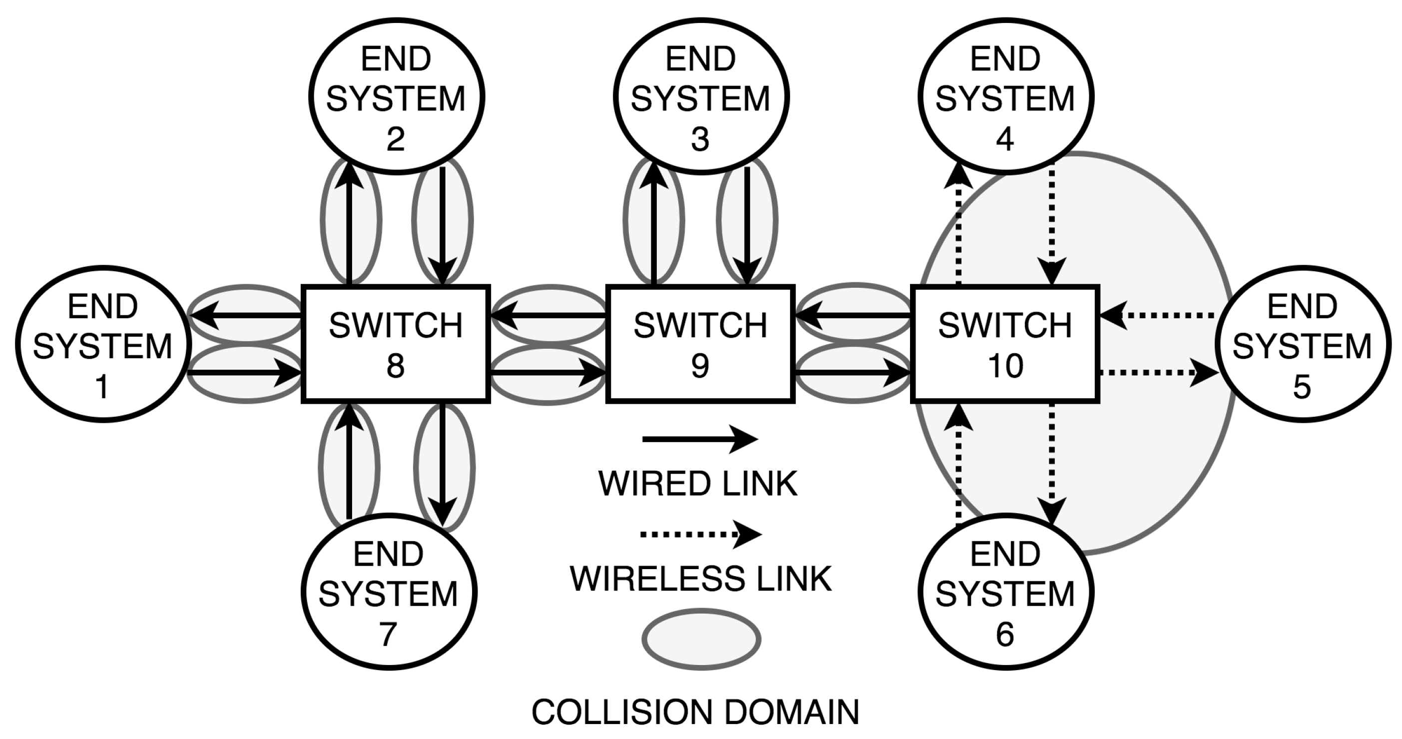
We define a multi-hop network as an undirected graph $G=(V,E)$, where the vertices V represent witches and end systems, and the edges E represent bi-directional connections between vertices. Data is exchanged between vertices through frames, with F denoting the set of all the frames of the network. Particularly, two vertices $v_x,v_y\in V$ can exchange frames if they are connected to an edge and only if at least one of the vertices is a switch. Besides, end systems are only allowed to have one connection. In contrast, switches are permitted to connect to multiple switches and end systems. For notational convenience, we will represent each edge by two directional links, one for each direction, where we denote the set of all links as L. The link $(v_x,v_y)\in L$ designates the connection from vertex x to vertex y, while $(v_y,v_x)\in L$ denotes the opposite direction in the same edge, from vertex y to vertex x. Each link $l\in L$ characterizes its capacity $C_l$, measured in Bps (bytes per second).

Additionally, a communication link can be either wired or wireless. A link is considered to be wired if there exists a physical connection between the vertices through a full-duplex cable, such that transmission of frames in both directions is possible simultaneously. In wireless links, wireless access points (WAP), located in the corresponding switches and end systems, transmit the frames without the need for a physical connection. We denote the set of all wired links and the set of all wireless links $L_w$ and $L_x$, respectively. Note that $L=L_x\cup L_w$, and $L_x\cap L_w=\varnothing$.

A distinctiveness of wireless links, in contrast to wired links, is that transmissions can collide with other wireless transmissions in the proximity, as they share the same medium. To avoid frame losses due to such collisions among them, we define a collision domain $\mathit{CD}$ as:

$$\mathit{CD}=\{(v_{x_1},v_{y_1}),(v_{x_2},v_{y_2}),\dots ,(v_{x_n},v_{y_n})\}\subseteq L$$

(1)

A $CD$ includes n (wireless) links that are not allowed to transmit at the same time due to the feasibility of a collision. Moreover, it is possible for a wireless link to belong to multiple collision domains. In the case of wired links, we assume that each forms its collision domain with a single link.

One of the main drawbacks of wireless communication is its low reliability caused by external interferences. Temporal redundancy is used to increase its reliability, which means that several replicas of a frame are transmitted, each one separated by the so-called inter transmission time ($ITI$). Temporal redundancy increases the probability of receiving at least one replica correctly, and it is necessary for links with a higher error rate [17]. In our model, we will assume that the total number of replicas is fixed ($=k$) for all the wireless links.

For each switch in the network, we define the parameter hopdelay, which indicates the time the frame is stored in the switch before it can be relayed. We also define the parameter maxmemory, which is the maximum time that a frame can be stored in a switch before being forwarded. Both parameters give a lower and upper bound regarding the processing and memory capabilities of the switches. Without loss of generality, in this work, we assume that hopdelay and maxmemory is the same for all switches.

2.2. Traffic Model

An end system sender can transmit information over frames to one or multiple end systems receivers. The sequence of links between the sender and a receiver defines the data flow path p:

$$\begin{array}{c}p=[(v_s,v_{s+1}),\dots ,(v_{r-1},v_r)]\hfill \end{array}$$

(2)

where $v_s$ is the sender and $v_r$ is the receiver. We define the tree path of a frame f, denoted as ${\mathit{TP}}_{\mathit{f}}$, as the union of all data flow paths from the sender of f to each one of its receivers. In our model, we select the data flows as the shortest path between end systems. However, it is possible for the designer to specify any data flow to connect end systems. We illustrate this concept with an example. Figure 1 shows a hybrid network with seven end systems, three switches, 12 wired links and six wireless links belonging to the same collision domain.

Formally, a frame f is defined by the tuple:

$$f=\langle {\mathit{T}}_{\mathit{f}},{\mathit{D}}_{\mathit{f}},{\mathit{L}}_{\mathit{f}},{\mathit{TP}}_{\mathit{f}}\rangle ,$$

(3)

where ${\mathit{T}}_{\mathit{f}}$ is the frame period, strictly periodic, ${\mathit{D}}_{\mathit{f}}$ is the frame deadline, ${\mathit{L}}_{\mathit{f}}$ is the size of the frame (measured in bytes), and ${\mathit{TP}}_{\mathit{f}}$ is the tree path as defined above.

Given a set of frames F, they determine the schedule hyper-period (${\mathit{T}}_{\mathit{F}}$) as the least common multiple of the periods of the frames: ${\mathit{T}}_{\mathit{F}}=LCM(\forall {\mathit{T}}_{\mathit{f}}\in F)$. Within the hyper-period, a frame might need to be transmitted more than once: the number of frame instances of frame $f\in F$ (denoted ${\mathit{N}}_{\mathit{f}}$) within the hyper-period is calculated as ${\mathit{N}}_{\mathit{f}}=\frac{{\mathit{T}}_{\mathit{F}}}{{\mathit{T}}_{\mathit{f}}}$. Note that when this is combined with the temporal redundancy mechanism for wireless links described in Section 2.1, each frame instance is transmitted as k replicas.

We will denote as ${\Delta }_f^l$ the time needed to transmit frame $f\in F$ over link $l\in L$, calculated as ${\Delta }_f^l=\frac{{\mathit{L}}_{\mathit{f}}}{{\mathit{C}}_{\mathit{l}}}$.

2.3. Schedule Synthesis Problem

The goal of the time-triggered schedule is to designate, for each link, the transmission time for each frame instances and replicas, that the network needs to transmit within the hyper-period. For this purpose, we define the function ${\Phi }_{\mathit{f}}$, called Offset, for each frame $f\in F$ as follows:

$${\Phi }_f:[1,{\mathit{N}}_{\mathit{f}}]\times {\mathit{TP}}_{\mathit{f}}\times [1,k]\to {\mathbb{R}}^{+}\cup \{*\}$$

(4)

where ${\Phi }_{\mathit{f}}(i,l,k)=t$, with $t>0$, indicates that the node starts the transmission of the k-th replica of the i-th instance of frame f over the link l at time t. If the node does not transmit a k-th replica of the i-th instance of frame f over link l, we denote it as ${\Phi }_{\mathit{f}}(i,l,k)=*$. Recall that in the TT paradigm, only scheduled frames are transmitted.

By our definition of the frame set, a node cannot transmit a frame f over a link that does not belong to its tree path (${\mathit{TP}}_{\mathit{f}}$). Additionally, if a link is wired, there is no need to transmit replicas (this assumption of our system model could be easily relaxed, without causing any important change in the scheduler.), so for all $l\in {\mathit{L}}_{\mathit{w}}$ and $k>1$, ${\Phi }_{\mathit{f}}(i,l,k)=*$.

Other characteristics of ${\Phi }_{\mathit{f}}$, derived from some TT protocol design decisions [6,17], are: (1) Consecutive frame instances are scheduled with a separation equal to the frame period: ${\Phi }_f(i+1,l,k)={\Phi }_f(i,l,k)+T_f$; for $1\le i\le N_f-1$; and (2) Consecutive frame replicas are scheduled with a separation equal to $ITI$: ${\Phi }_{\mathit{f}}(i,l,k+1)={\Phi }_{\mathit{f}}(i,l,k)+ITI$; for $k>1$ and $l\in L_x$.

Given the previous definitions, we can now establish the schedule synthesis problem. Given a set of frames F, synthesizing a schedule involves finding a valid (concerning the properties stated above) assignment to ${\Phi }_{\mathit{f}}$ such that the schedule does not violate the constraints of F.

Since finding offset values in the real domain is particularly complex, we use the notion of a slot [18], a discretization of the transmission time into natural numbers. We define the discrete offset function as follows:

$${\Phi }_{\mathit{f}}:[1,{\mathit{N}}_{\mathit{f}}]\times {\mathit{TP}}_{\mathit{f}}\times [1,k]\to {\mathbb{N}}^{+}\cup \{*\}$$

(5)

A common practice for reducing the complexity of the problem is to define a slot size ($ssize$) as the time to transmit the largest frame in the slowest link, and hence each slot contains a frame transmission. However, due to the introduction of wireless links, commonly much slower than wired links, we obtain excessively large size slots in which many frames only occupy a minute fraction of the total slot size. Creating such schedules would yield a very inefficient use of the available bandwidth and should be avoided. We instead decided to define a much smaller slot size, one nanosecond, and cope with the added complexity so that we obtain more realistic and efficient schedules.

Once we define $ssize$, we can normalize the transmission delay of each frame as follows: ${\delta }_{\mathit{f}}^l=\lceil \frac{{\Delta }_{\mathit{f}}^l}{ssize}\rceil$. Other variables are also trivially normalized in a similar manner.

3. SMT Schedule Synthesis

In this work, the scheduling problem is modelled with linear integer constraints. Constraints are asserted into a constraint solver, in our case, a satisfiability modulo theory (SMT) solver, that implements linear integer logic. SMT is an extension of the satisfiability boolean problem (SAT) to handle first-order logic. SMT solvers are tools capable of finding the satisfiability or unsatisfiability of a set of constraints and, in the case that a satisfiable assignment is found, it also returns a model with the assignment as proof of such satisfiability. For the schedule synthesis problem, the solver returns a model with the assignment of all offsets (${\Phi }_f$ for each frame $f\in F$) that guarantees that the constraints hold. If the network is not schedulable for the given set of frames and constraints, the SMT solver will notify unsatisfiability.

In the following, we present our formulation as linear integer constraints. It is coherent with the formulation given in [13], but it has been extended with two constraints that correspond specifically to wireless communication (the replica and avoid-collisions constraints):

Frame Period Constraints:

Allocating a frame while meeting its strict periodicity constraint consists of two parts: first, we assign the first instance satisfying its period range, then we can allocate the following instances with a transmission distance equal to its period. For the first part, we must ensure that all links in the tree path are in the range $(0,T_f]$:

$$\begin{array}{c}0<{\Phi }_f(1,l,1)+{\delta }_f^l\le T_f\hfill \end{array}$$

(6)

The following frame instances are determined from the first frame instance and the period:

$$\begin{array}{c}{\Phi }_f(i,l,1)={\Phi }_f(1,l,1)+(i-1)\times T_f\hfill \end{array}$$

(7)

Frame Deadline Constraint:

To provide a frame deadline shorter than the period ($D_f<T_f$), we need to limit the range of the first instance period constraint:

$$\begin{array}{c}0<{\Phi }_f(1,l,1)+{\delta }_f^l\le D_f\hfill \end{array}$$

(8)

Replica constraints:

These constraints are applied to the wireless links, where temporal redundancy is used. $ITIsize$ defines the distance of the $ITI$ presented in Section 2.1:

$$\begin{array}{c}{\Phi }_f(i,l,k)={\Phi }_f(i,l,1)+(k-1)\times ITIsize\hfill \end{array}$$

(9)

Avoid-Collision Constraints:

In time-triggered communication, it is not possible to transmit more than one frame through the same collision domain at the same time. Hence, this constraint will ensure that no transmission is allowed to start while another transmission is still in progress within the same collision domain. Moreover, it also ensures that no transmission is allowed if it cannot be finished before another scheduled transmission starts. Therefore, $\forall f\in F$, $\forall l\in L$:

$$\begin{array}{c}\mathrm{If} {\Phi }_f(i,l,k)=t,\mathrm{with} l\in C_j,\mathrm{then} \hfill \\ \nexists \{g,m,x,y\},\mathrm{with} g\in F,m\in C_j,x\in (1..N_g),y\in (1..K)\hfill \\ \mathrm{such} \mathrm{that} {\Phi }_f(i,l,k)-{\delta }_g^m\le {\Phi }_g(x,m,y)\le {\Phi }_f(i,l,k)+{\delta }_f^l\hfill \end{array}$$

(10)

Ensure-Causality Constraints:

Frame dataflow paths need to follow a sequenced order of links from the sender to the receiver. This means that a switch cannot relay a frame if it has not previously received the frame. So for every pair of consecutive links $(v_x,v_y),(v_y,v_z)\in {\mathit{TP}}_f$ in a datapath:

$$\begin{array}{c}{\Phi }_f(1,(v_y,v_z),1)-{\Phi }_f(1,(v_x,v_y),1)\ge \mathit{hopdelay}\hfill \end{array}$$

(11)

Note that once this constraint is defined for the first replica of the first frame instance, the subsequent instances and replicas also fulfil the property transitively, due to the period and replica constraints.

Avoid-Buffer-Overflow Constraints:

The schedule also needs to respect the memory limitations of the intermediate switches. For every pair of consecutive links $(v_x,v_y),(v_y,v_z)\in {\mathit{TP}}_f$ in a datapath:

$$\begin{array}{c}{\Phi }_f(1,(v_y,v_z),1)-{\Phi }_f(1,(v_x,v_y),1)\ge \mathit{memory}\hfill \end{array}$$

(12)

As with the previous constraint, there is no need to define the same property for the next frame instances and replicas, since they will satisfy the property transitively.

Simultaneous-Relay Constraints:

Some protocol implementations require the switch to relay a multicast frame through multiple links at the same time. In particular, this happens whenever two links in the same tree path share the same predecessor. For any pair $(v_x,v_y),(v_x,v_z)\in {\mathit{TP}}_f$:

$$\begin{array}{c}{\Phi }_f(1,(v_x,v_y),1)={\Phi }_f(1,(v_x,v_z),1)\hfill \end{array}$$

(13)

End-to-End Latency Constraints:

For certain communications, the time elapsed between the start of the frame transmission in the sender until the reception at each one of the receivers needs to be bounded. Even if this end-to-end delay is, in practice, bounded by the Avoid-Buffer-Overflow constraint, it is possible to restrict it even further with the parameter $endtime$ as follows.

$$\begin{array}{c}{\Phi }_f(1,(v_{r-1},v_r),1)-{\Phi }_f(1,(v_s,v_{s+1}),1)<\mathit{endtime}\hfill \end{array}$$

(14)

Application Constraints:

In this article, we assume that tasks and frames are scheduled separately. However, frames may have inter-dependencies that are inherited from the tasks schedule. There is a need to provide a mechanism that allows taking these dependencies into account when generating the network schedule. We solve these dependencies with the definition of application constraints such that a frame $f\in F$ can only be received exactly after some time (indicated by the parameter $\mathit{app}\_\mathit{time}$) has passed since the reception of another frame $g\in F$.

$$\begin{array}{c}(v_{r-1},v_r)\in {\mathit{TP}}_f,(v_{r-1}^{\prime },v_r^{\prime })\in {\mathit{TP}}_g:\hfill \\ {\Phi }_f(1,(v_{r-1},v_r),1)={\Phi }_g(1,(v_{r-1}^{\prime },v_r^{\prime }),1)+\mathit{app}\_\mathit{time}\hfill \end{array}$$

(15)

Note that to map applications to frame transmissions, the constraint is defined only for the last link of the tree path, while all the predecessor vertices will fulfil it transitively.

4. Four Enhancements to the Segmented Approach

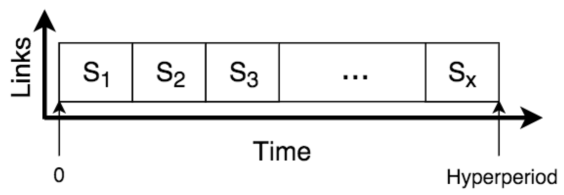
We originally developed the segmented approach to overcome some important scalability issues that SMT synthesis presented when trying to schedule large networks. This approach follows a divide-and-conquer strategy: instead of trying to solve the whole schedule at once, we divide the schedule into small segments that are scheduled separately, as shown in Figure 2. The complete schedule S is partitioned into segments $S[a;b]$; where a and b are the times of the first and last slot of S, respectively. The segments are non-overlapping and jointly contain all the time slots from the start of the schedule to the end of the schedule, the hyper-period. The first results with this approach were very promising [19,20].

The procedure works as follows. After the schedule is divided into segments, we try to allocate as many frames as possible in a single segment to produce a scheduled segment. A random number of frames is selected, and their constraints are introduced into the SMT logical context, limiting its offsets to values inside the assigned segment. If the SMT solver returns a valid schedule, we can try to repeat the scheduling of the segment with more frames until we get unsatisfiability. Once we get this result, the previous valid scheduled segment is selected and committed, and the process is repeated with the next segment until all frames are scheduled. If all segments are scheduled, but we still have frames left to be allocated, no valid schedule has been found.

However, the segmented approach presents some limitations when applied to TT schedules:

• The complexity of scheduling a segment can still be too high for SMT synthesis. Moreover, the number of frames that can be effectively allocated in a segment is not known beforehand, leading to excessive delays when trying to fully allocate frames in a segment.
• Backtracking in huge state space problems is impractical. When solving a problem by steps, bad decisions may prevent us from finding a solution. For instance, allocating a frame that is a predecessor of another frame before the latter is allocated, so their temporal relationship may not hold. Backtracking to the point where these problems can be solved is highly inefficient.
• Frames in different segments may not be independent from each other, creating dependencies between consecutive synthesis of segment schedules. Not proper handling of these dependencies leads to incorrect schedules, in which inter-segment dependencies are violated.
• The schedule obtained is highly fragmented. Not only we are missing many possible and potentially better solutions, but we also obtain a schedule with many free slots between segments. This needs to be managed to improve the bandwidth utilization and is particularly important for networks having links of disparate capacities.

In this Section, we discuss each problem in depth and describe the solution that has been adopted. The evaluation of these new methods will be presented in Section 5.

4.1. Incremental Approach

Synthesizing a segment schedule with a one-shot SMT solver approach is highly inefficient. First, finding the exact number of frames that can be allocated in the segment is a trial and error approach. Second, detecting that the number of frames is too large for the segment could incur a significant delay. Recall that to prove satisfiability, the SMT solver only needs to find a valid assignment of the constraints, but to prove unsatisfiability, all the possible combinations must be checked, which, in some cases, is excessively time consuming.

To simplify and speed up the scheduling of a segment, we apply an incremental approach. Instead of having a trial and error of the number of frames possible in the segment, this approach gradually introduces additional frames into the segment, until the segment is full and the solver returns an unsatisfiability result.

The algorithm can be seen in Listing 1. The incremental approach receives the index to the list of frames that remains to be scheduled. The main loop is executed (line 3) and repeated until no more frames can be allocated in the segment. For every iteration, the algorithm chooses a number $stepsize$ of frames and tries to schedule them together. The $stepsize$ value has a significant impact on the performance because it concerns the number of constraints solved in every iteration. In line 6, all the constraints of the selected frames are added into the logical context to be satisfied. Also, in lines 7 and 8, a loop over the frames scheduled in the previous iterations is executed to add the avoid-collision constraints (see Section 3). Once all the frames are asserted into the logical context, the solver checks them (line 9). If the context is satisfiable, the returned model contains the offset values of the new scheduled frames. The obtained offsets are then read and their values are set as fixed with the assertion of the constraints described in lines 13 and 14. Finally, the algorithm increases the frame index, and the loop is repeated. If the context is unsatisfiable, the segment is considered full, and the index and model of the previous iteration are returned. Finally, the offset values of the scheduled segment are stored, and the scheduling of the next segment can be started.

4.2. Frame Preprocessing

The order in which our method allocates frames into the segments considerably influences the likelihood to find a valid schedule. Traditionally, the order was not considered as we could schedule all frames at the same time or we could always use a backtracking technique to account for unsatisfiable allocations. Unfortunately, for the segmented approach and huge state space problems, backtracking segments can be highly inefficient as there exist many invalid frame sequences. This is due to higher-level relations, application constraints, among frames that need to wait for other frames transmissions. Our solution implements a modified earliest deadline first (EDF) algorithm that takes into account the application constraints. The literature [19] shows that such strategies avoid the need for backtracking, and they can handle a high number of application constraints without presenting scalability issues. We are aware that the implementation of a backtracking that extends beyond the segment size would help us to schedule instances with very high utilization. However, we experimentally found out that our scheduling problems rapidly turned out to be too complex for the solver, without any real improvement over a solution without backtracking.

Our solution calculates what we name accumulated app_time, defined as the maximum recursively time that any of its children frames has to wait to be transmitted. This value is then subtracted from their frame deadlines to allow all the children frames of the application constraint to procure enough time to be scheduled, such that all deadlines are satisfied. Observe the example in Figure 3, where we show the app_time at the top left of each frame, represented by a box. The value inside the box is the value subtracted from the frame deadline, calculated as the app_time propagated from all its children; e.g., should frame $f_7$ have a deadline of 1000, its new deadline would become 1000 − 420 = 580. We obtain 420 as the longest path of the whole tree, the one to the right with 250 + 170 = 420.

Once this parameter is calculated for each frame, it becomes the ordering index of the frames for the scheduling problem. Frames with shorter accumulated app_time are fed to the scheduler before frames with larger accumulated app_time. This ensures that no backtracking is required and reduces the schedule synthesis time.

4.3. Segment Preprocessing

Frames that have been scheduled in previous segments may still have constraints that influence the remaining schedule. These inter-segment constraints may be of two types: period and application constraints. Period constraints dictate the distance between different frame instances that appear in different segments, while application constraints dictate that a frame has to wait for a parent frame that was scheduled in a previous segment.

For the new segment to be able to satisfy inter-segment constraints, we need to keep previous inter-segment constraints satisfied, while solving the segment independently. We introduce an algorithm in Listing 2 that keeps track of these constraints once they have been already allocated. The fix offsets algorithm iterates over all previously scheduled frames and examines if any of their instances appear in the segment to be currently scheduled; if it does, it adds a new constraint capturing its transmission time. In the case of application constraints, the algorithm checks if any of the already scheduled frames is the parent of a frame that is to be scheduled in the segment, and also adds a constraint capturing the parent’s transmission time.

Thanks to this mechanism, whenever the synthesis of a new segment schedule starts, we load the constraints caused by previous segments that do affect the current segment, such that they are considered by the solver.

4.4. Segment Efficiency

Segmentation induces a certain level of internal fragmentation. In this section, we show how the compactness of the schedule can be improved employing a new type of constraint. We also introduce some small modifications to reduce the time needed to synthesize schedules.

4.4.1. Variable Segment Size

The size chosen for the segment has a substantial impact on the performance and segmentation of the schedule. Large segment sizes allow for more frames to be allocated into the segment, yet the time needed to schedule it also increases. The opposite situation happens with smaller segments, where the time to schedule decreases but it allocates fewer frames and increases the number of free spaces left in the segment. Moreover, a too small segment size might cause a frame to not fit in the segment, and therefore, the segmented approach would be unsuccessful.

To find a balance between segmentation and synthesis time of the segment, we aim to find a larger segment size that is still manageable for the incremental approach. This segment size is solver feedback dependent and can be implemented in many different configurations. The main idea is to listen to the solver to dictate the segment size. For example, defining a desired range of time or range of frames to be scheduled in each segment. The implementation is simple: if we choose a range of time, at the start of each segment, if the previous segment takes a smaller time than a user-defined threshold, we increase the segment size. If it takes longer than the threshold, we decrease the size.

4.4.2. Relaxed Constraints

A drawback of the segmented approach, compared to other approaches, is that it trades synthesis speed with the likelihood to find a schedule of a network with very high utilization. The main difference is that the segmented approach does not allow allocating a frame between segments, and thus, disregards some possible combinations.

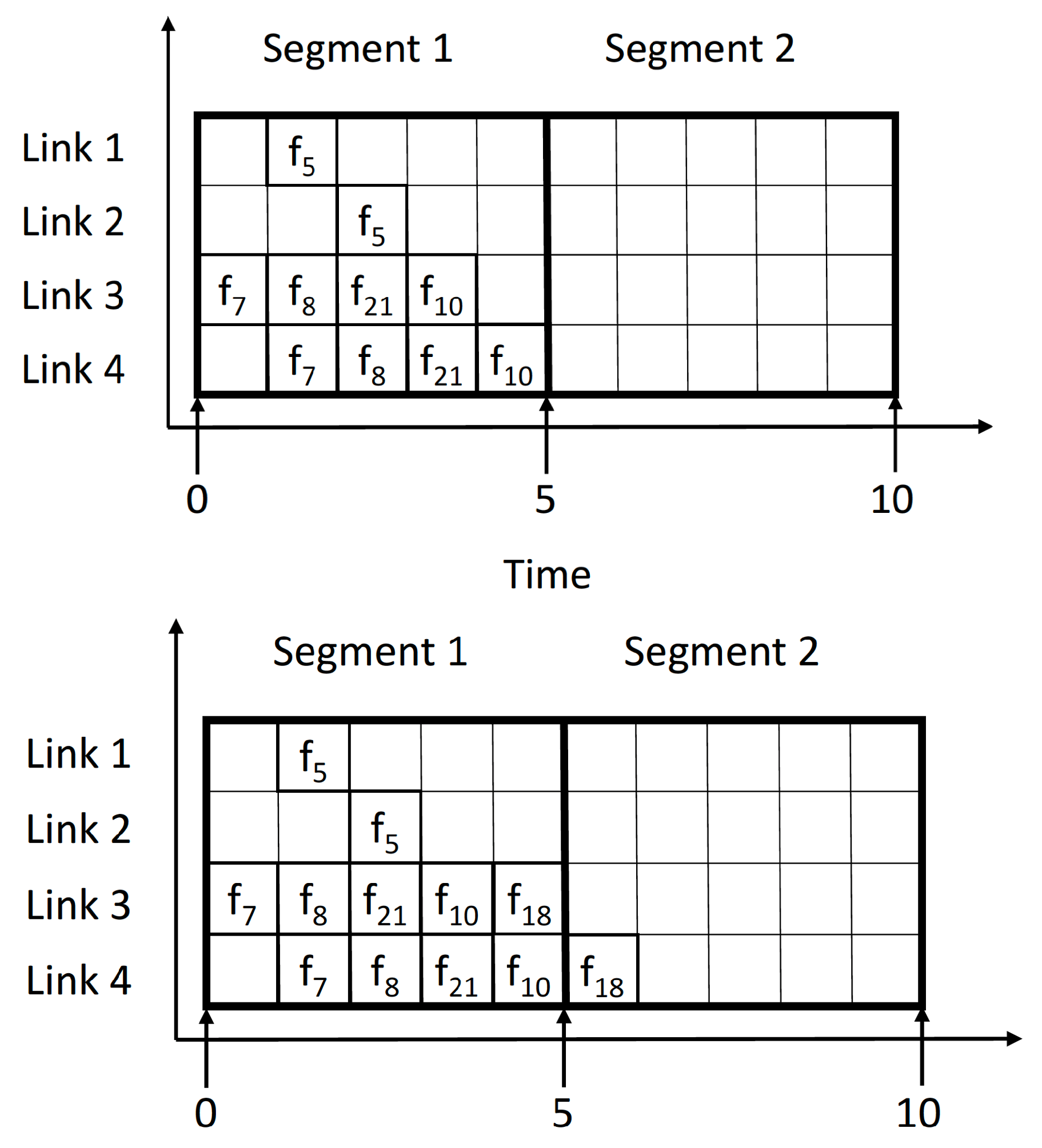
We introduce what we call relaxed constraints to try to fill every segment as much as possible. The idea behind this concept is to allow frames that do not entirely fit in the segment, to be partially allocated in the subsequent segment as well. Letting frames be scheduled in either the current or the next segment, allows allocating slots that would otherwise be left unused. This approach can be useful in reducing schedule fragmentation; for instance, if a link is saturated within a segment while the other links are still unoccupied. Instead of terminating the segment scheduling because a frame has to (but cannot) use this already-saturated link, the algorithm would allocate this frame within the next segment while additional frames can still fit the current segment. Let us illustrate this idea with the example in Figure 4. We assume that our scheduler allocates a frame one by one and we are scheduling the first segment. The links 3 and 4 are full, while the links 1 and 2 could fit more frames similar to frame 5. If we are trying to schedule the frame 18, which also needs to be allocated in links 3 and 4, it does not necessarily fit in segment 1, and the segmented approach will set the segment as full and start scheduling frame 18 in segment 2. However, if we allow frame 18 to be scheduled in either of the two segments, the segment is not set as full, and we can still schedule more frames similar to frame 5 in the first segment.

To implement the relaxed constraints, we need to review the constraints when we fail to schedule a frame in the segment. Whenever we get an unsatisfiable result, we try to schedule the same frame again but allowing to place them in either the current segment or in the next one. We can do it by replacing the frame period constraints with the following:

$$\begin{array}{c}\hfill S^{(a,b]},S^{(b,c]}:a<{\Phi }_f(1,l,1)+{\delta }_f^l\le c\end{array}$$

(16)

If the scheduler with the relaxed constraints finds a schedule, we continue allocating frames only within the current segment. Otherwise, if the solver cannot find a solution after applying the relaxed constraints, we establish the segment as fully scheduled and start scheduling the next segment. It is essential that when scheduling the next segment, we handle the offsets of the frames with relaxed constraints in our segment preprocessing algorithm, adding the offsets of frames that the solver scheduled in the next segment.

5. Evaluation

The scope of this evaluation is to find the upper bound on the number of frames that the segmented approach can schedule in a reasonable time for different network sizes and traffic configurations. According to our industrial contacts, less than 5 hours is reasonable for scheduling a large network, we will use that figure as a reference. We also evaluate how the schedule segmentation is affected by our algorithms.

5.1. Baseline

Several studies have evaluated schedule synthesis algorithms for time-triggered networks, see, e.g., [12,13,21,22]. These studies consider networks of moderate sizes, in the order of tens of nodes and around ten switches, with less than a hundred dataflow links. The schedules are obtained for frame set sizes ranging from hundreds to two-thousand messages. Due to the differences between networks and the lack of standard metrics, it is difficult to compare the performance quantitatively. Steiner [13] introduced a unified measure called frame instances, which corresponds to the total number of frame transmissions in each link along the whole hyper-period. For the general case, this measure is a better indicator of the complexity of synthesizing the schedule of specific traffic over a network: the lower this number is, the simpler the synthesis becomes. In this paper, we will call this parameter transmissions in links, and we will use it for the evaluation of our algorithms. Existing approaches were able to synthesize schedules over 20,000 transmissions in links in less than 30 min [13]. We show in this evaluation that we can synthesize schedules with more than four orders of magnitude more transmissions in links, while not exceeding our 5 h time limit, and synthesizing schedules over ${10}^6$ transmission in links in less than 30 min.

5.2. Case Study

One can only hypothesize about what future large-scale real-time networks will look like in terms of size and topology. Our approach in this evaluation is to take an existing large-scale network and extend it with the features that are becoming prominent in the embedded domain. The starting point is the topology of a network implemented by MallorcaWifi in Platja de Palma, a wide tree topology that provides a free wireless connection in a large and very populated touristic area. This network has received much attention because of its size and high throughput (The Cisco press release about this case study can be found here: https://meraki.cisco.com/customers/hospitality-and-tourism/city-of-palma-de-mallorca).

Even if there are no hard real-time requirements in this network, and it is almost entirely wireless, we consider that the number of nodes and the topology is indicative for future networks with real-time requirements. The network is composed of 44 switches, 81 end systems and a total of 248 data flow links, with a maximum path distance of 10 switches between end systems. In the original network, most of the links are wireless; however, in real-time networks, it is unlikely that wireless communication will be used for the backbone links. For this reason, we choose to define all backbone connections as wired and have 20% of the end systems connected by wireless (16 end systems, and 32 wireless links included in 6 collision domains). We distinguish three different link types in the network: a wired backbone connection between switches at 100 MB/s, a wired connection from a switch to an end system at 50 MB/s and a wireless connection from a switch to an end system at 20 MB/s.

Concerning the data traffic, frames are sent evenly distributed among all the end systems. Periods, deadlines and frame sizes are defined in four different traffic classes. Furthermore, we also differentiate four other types of traffic classes, related to the characteristics of the frame receivers:

• Single frames: whenever an end system sends a frame to another randomly selected end system.
• Multicast frames: whenever an end system sends a frame to a random number of end systems.
• Local frames: whenever an end system sends a frame to all end systems connected to the same switch it is connected. These frames have a path distance of two data flow links.
• Broadcast frames: whenever an end system sends a frame to every other end system in the network.

After permuting all the classes, we obtain 16 different mixes of traffic classes that end systems can send. The configuration of the traffic classes is finely tuned in two different utilizations in the network: low utilization (LU) and high utilization (HU). An LU network will have a maximum link utilization in the range of 40% to 50%, which means that at least one link will have its utilization in such range and no link will have higher utilization than 50%. Meanwhile, a HU network will have a maximum link utilization in the range of 70% to 80%. We decided the HU maximum link utilization as we consistently cannot schedule networks with more than 85% maximum link utilization when all the links are wired and have the same speed. However, we manage to schedule up to 99% link utilization when there is a presence of wireless links.

As for the values defined in constraints, which are described in Section 3, we made the following decisions. We model application constraints as a tree with a maximum depth of 3 and up to three successors. The time that a frame must wait as a consequence of an application constraint is randomly selected within the range [100–300] $\mathsf{\mu }$s. Frames transmitted in wireless links are retransmitted one extra time, making a total of two replicas, with $ITI$ = 50 $\mathsf{\mu }$s. Switches relay frames 1 $\mathsf{\mu }$s after the entire frame is received (hopdelay parameter) and a frame cannot stay more than 10 $\mathsf{\mu }$s (memory parameter) within a switch. We do not show any evaluation of the constraint parameters as we found that only the number of replicas significantly affects the synthesis time. We considered the number of replicas to have a significant correlation with the utilization, but with a much lower impact.

The improvement of the segmented approach is set with relaxed constraints activated. The variable segment size algorithm will start with 1 ms, but it can increase or decrease in steps of 500 $\mathsf{\mu }$s. Our threshold to increase or decrease will be the number of times that we call the SMT solver to find a segment. If we schedule the segment with less than three iterations in the incremental approach, we will increase the size. We will decrease it if we need more than ten iterations. The performance impact of these values will be evaluated at the end of this section.

Finally, we also created two additional network topologies to evaluate larger networks, including more evenly distributed traffic, with a resulting total of three networks topologies evaluated:

• Actual network: the previously presented network composed of 44 switches, 81 end systems and a total of 248 data flow links, with a maximum path distance of ten switches between end systems. 20% of the end systems are connected via wireless with six collision domains.
• Large network: composed of 133 switches, 241 end systems and 746 data flow links, with a maximum path distance of 20 switches between end systems; 20% of the end systems are connected via wireless with 24 collision domains.
• Wired network: the topology is the same as the Actual network, but all its links are wired reaching a speed of 100 MB/s. We aim to evaluate a more evenly distributed traffic network with a more balanced utilization among the links. The Actual network has a bottleneck in the wireless communication becoming saturated at 10% network utilization for HU, while the Wired Actual network with HU becomes saturated at a network utilization of 50%.

The constraints were fed to the SMT solver Yices 2.5 and solved applying the linear integer arithmetic background theory, which is the theory that provided the best performance for schedule synthesis in a previous study [19]. The incremental approach scheduling the segments allocates one frame at each iteration. The algorithms are programmed in Python 3 but executed with PyPy3 to increase performance. The evaluation was run on an Intel Xeon of 2.4 GHz, 14 GB of RAM with Ubuntu 14.04 LTS.

5.3. Time Performance

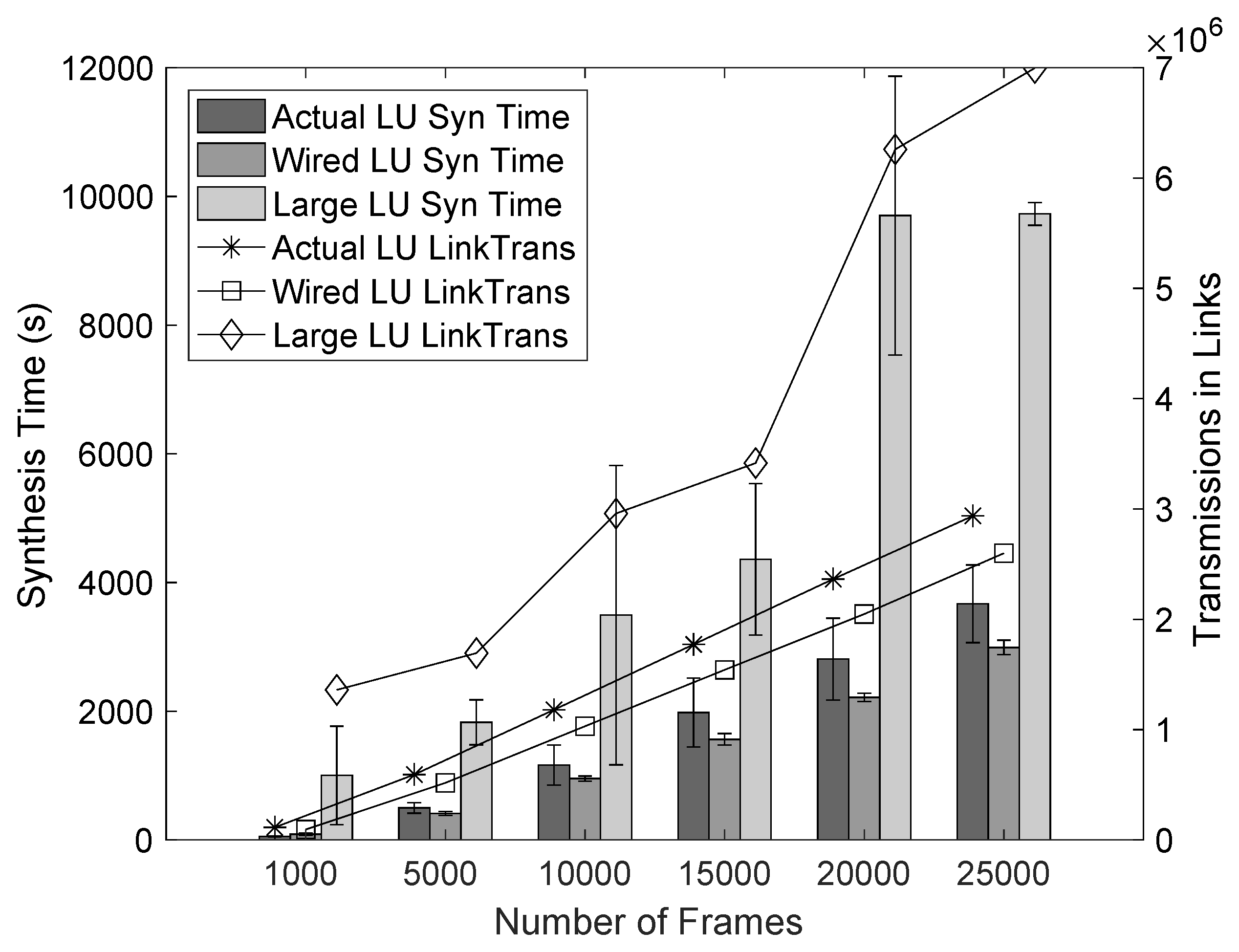
In Figure 5, we present the synthesis times for all three networks with LU containing a different number of frames. We can see that more frames correlate to more transmissions in links, which increases the synthesis time as it also increases the number of constraints to be solved to obtain the schedule. If we compare the large network with the actual network, the large network has more transmissions as its complexity increases due to multicast and broadcast frames and due to longer paths, which require more transmissions, and therefore, need more time to be scheduled. The Wired network gives a lower number of transmissions and shorter synthesis time, compared to the actual network, due to not having to transmit any replicas. We can also see that the synthesis time variation is smaller as the traffic is more evenly distributed and does not present hard segments to solve as opposed to the Actual network with wireless constraints. The most important information we can extract is the approximately linear to the synthesis time. We conclude that segmentation linearizes the time needed for scheduling at least in the considered cases.

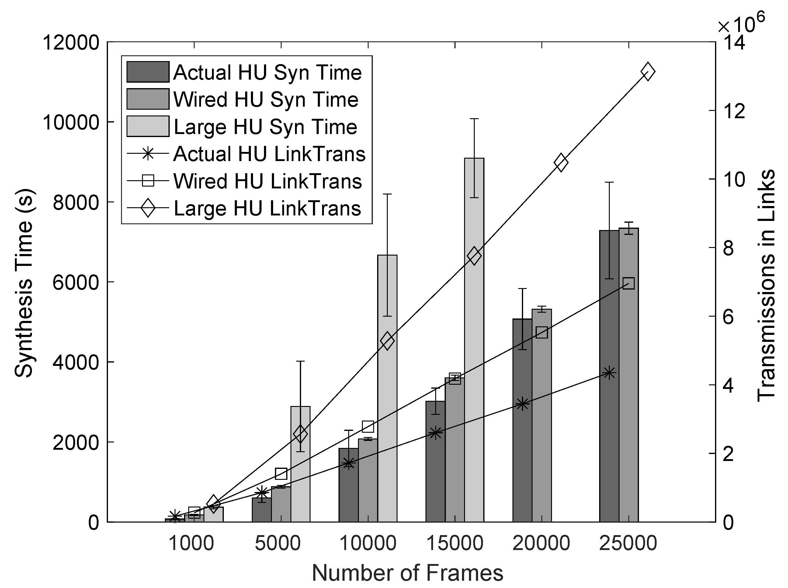
In Figure 6 we further evaluate how the synthesis times and transmissions in links are affected for HU networks. We can see that both transmissions in links, and therefore, synthesis times are notably increased compared with Figure 5. This situation occurs as all networks now have more traffic and require extra constraints to be scheduled. Also, note that for higher utilization, synthesis time increases much more, concerning the transmissions in links, than it does in the previous figure with lower utilization. Although we do not show it, for higher utilization, the segmented approach needs more time to create and feed the constraints to the SMT solver, which explains the considerable increase in synthesis time. However, the synthesis time with different frames remains approximately linear. Note that, for the Large network, we do not show any values for more than 20,000 frames, as the machine ran out of memory due to the high memory consumption of saving the objects containing the information of the schedule being solved.

5.4. Segmentation Performance

The segmented approach introduces fragmentation between segments, where many free slots are left at the end of the segment due to not being able to allocate an entire frame. The relaxed constraints aim to reduce the fragmentation, allowing frames to be scheduled in either segment instead of limiting a frame to a single segment.

The performance of our segmentation approach is difficult to measure when comparing with conventional algorithms due to two reasons. First, conventional algorithms cannot find a solution for large networks. Second, if we would reduce the network size to achieve a complexity that can be handled, the segmentation approach would solve it in a single segment, which does not provide any relevant results. However, it is evident that the segmentation approach might not find a schedule even if it exists, as pointed out in Section 5.2. To evaluate the effectiveness of relaxed constraints, we look at the schedule quality defined as the point in time in the schedule hyper-period when the segmented approach has allocated all first instances of all frames. A smaller completion time implies a higher quality schedule, as all frame first instances are compacted, leaving more free space for other traffic.

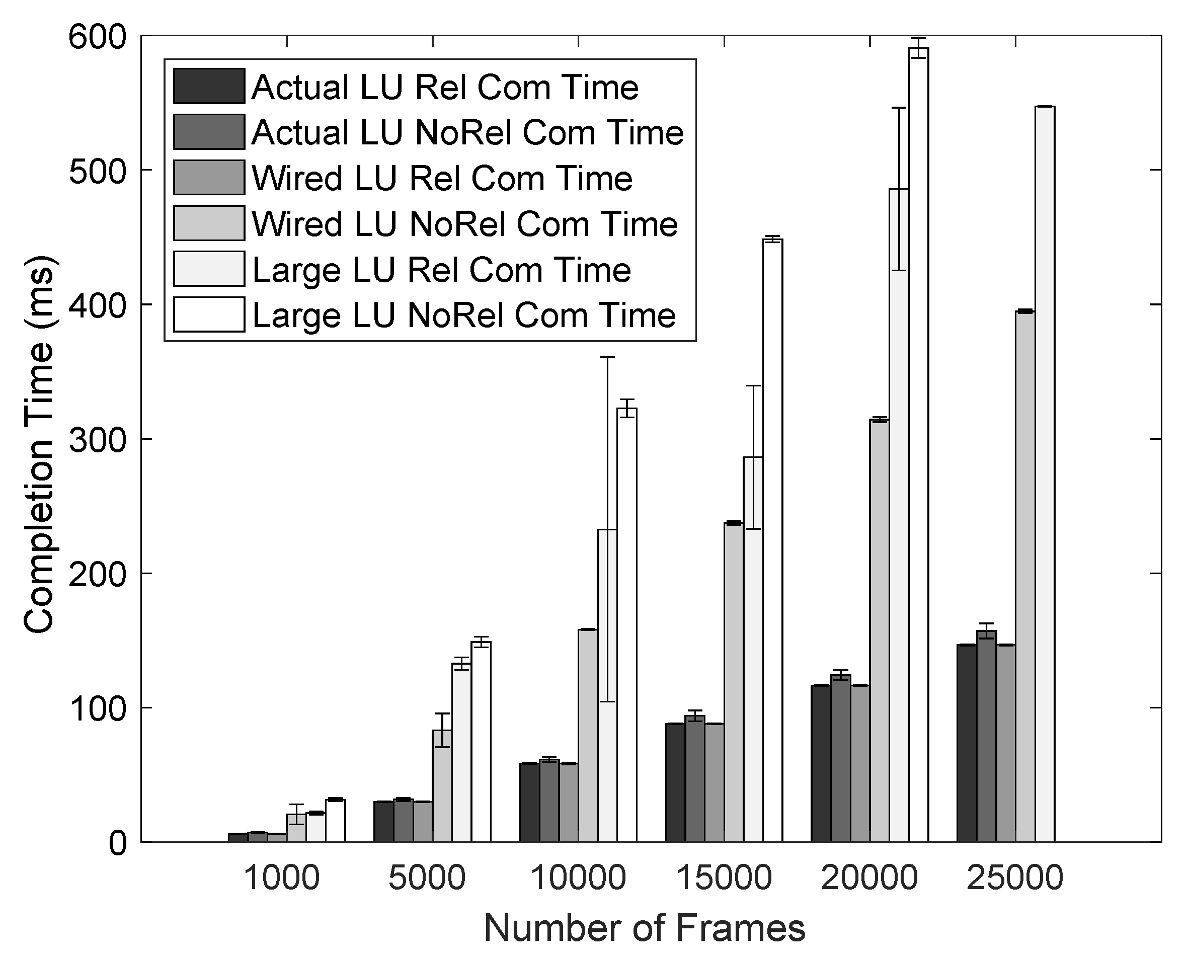
The relaxed constraints decrease the completion time for each of the considered networks. See Figure 7, especially for the Wired network, as the utilization of the links is more balanced, allowing to fill additional segments. However, for example, in the Actual network, the wireless links are filled much faster, and the segment scheduler needs to move to the following segment even though the wired links are still not entirely used.

The segment size also has an impact on the synthesis time and the completion time. Larger segments are harder to solve as the number of frames allocated in the segment increases. However, choosing a very small segment size makes it difficult for the scheduler to allocate a frame in the segment, as it may be too small to fit the whole frame. The variable segment size solves this problem, allowing the segment to increase or decrease in size to find a balance between performance and quality. 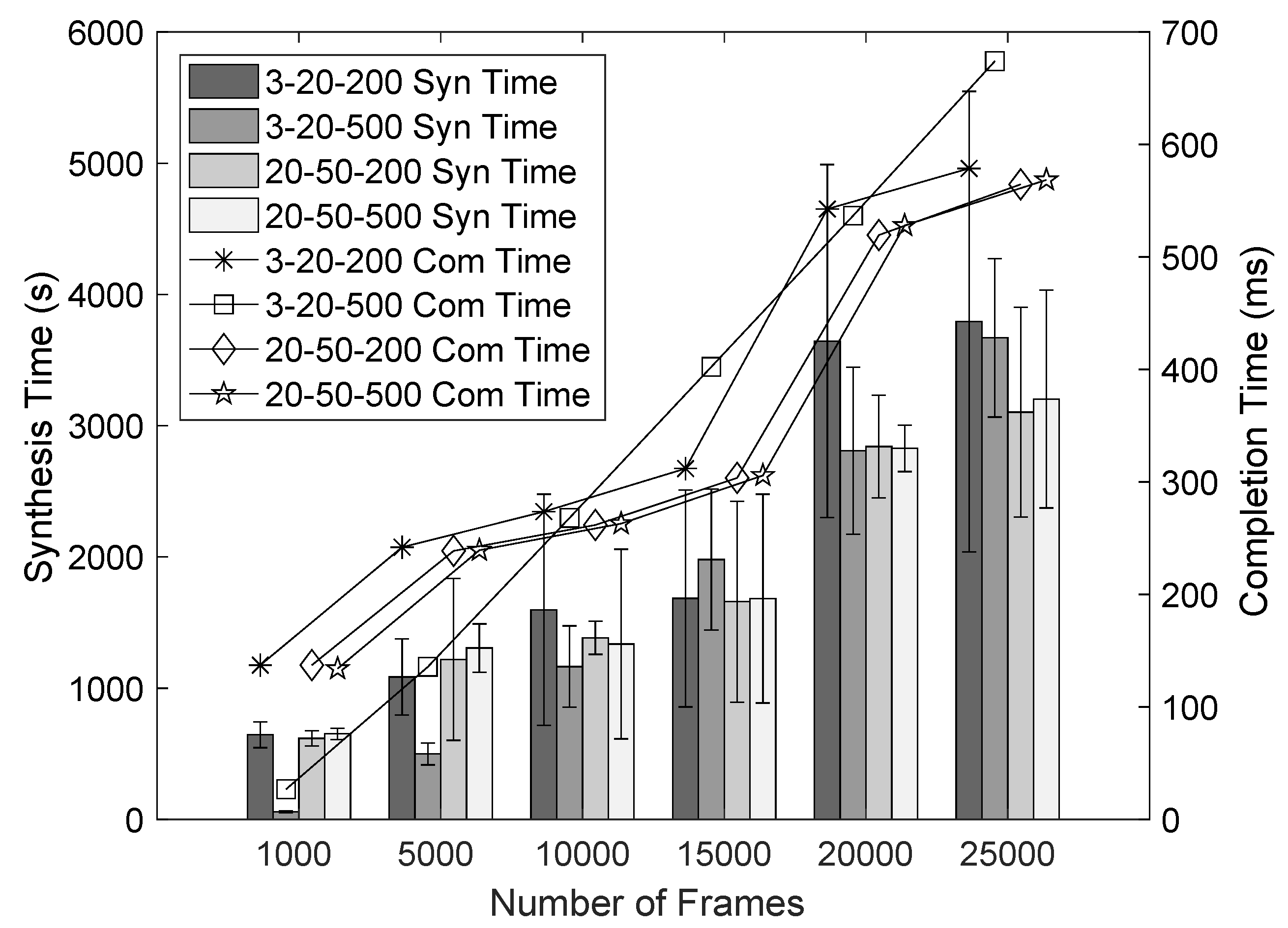In Figure 8 we evaluate different strategies depending on the number of solver invocations after which we change the segment size, as well as the $stepsize$ for such segment size change. We evaluate how it affects synthesis time and completion time in the Actual LU network for a different number of frames. For example, a 3-20-500 strategy means that the segment size will decrease by 500 $\mathsf{\mu }$s if it takes less than three invocations of the incremental approach to allocate the frames in the segment, or will increase with 500 $\mathsf{\mu }$s if it takes more than 20 invocations to allocate the segment fully.

We can see that the 3-20-500 strategy increases linearly in synthesis time and completion time, and outperforms the other strategies in scenarios with a small number of frames. However, for a higher number of frames, the 3-20-200 strategy outperforms the 3-20-500 strategy when it comes to completion time. The explanation is that the first strategy makes frequent but small changes to the segment size and seems to need more segments to change from a too large segment size to a smaller one, which decreases the completion time. We can also see that both the 20-50-200 and 20-50-500 strategies significantly outperform the other strategies in completion time and synthesis time for a larger number of frames. Since, with a larger number of frames, the segmented approach tends to group frames of the same size and periods. For a less-aggressive segment size change strategy, this allows better performance once a suitable segment size has been found. We can conclude that, for a small number of frames, it is better to use a strategy that changes the segment size often and in large sizes, while for a large number of frames, a strategy that does not present many changes performs better. However, these parameters may be very dependent on the considered network, and some tuning of the parameters may be needed in each specific case.

6. Related Work

Different techniques have been applied for the synthesis of time-triggered schedules. Satisfactory performance for small networks has been achieved with constraint programming (CP) solvers [23], integer linear programming (ILP) solvers [24], and satisfiability modulo theory (SMT) solvers [12,22]. However, scalability issues rapidly emerged with the increase in network size and traffic that required the integration of solvers with different heuristics and strategies. Hanzalek implemented a first step to prepare the tasks before scheduling using heuristics [25]. Craciunas and Serna developed a two-step method with SMT solvers in which the most resource-demanding frames are scheduled at the first step, while the remaining frames are allocated on top of the previously obtained schedule [21]. Other approaches combine more than two techniques, e.g., Biewer et al. conducted an interaction between an SMT solver interact and an answer set programming (ASP) approach to synthesize a network-on-chip schedule [26]. Steiner proposed an incremental approach implemented with an SMT solver that builds the schedule in iterations of only a group of frames, allocating them and selecting a new group of frames in every iteration until all frames are scheduled [13]. However, this approach presents saturation as the solver maintains the state of scheduled frames. The same approach was also used to schedule time-sensitive networks (TSN) [14]. Synthesizing schedules considering fault-tolerance has also been investigated. Avni et al. [27,28] generated schedules that allow reception of as many frames as possible even in the presence of faulty links: an SMT solver generates the schedule while a local protocol at each switch handles the retransmission of frames. All the previously mentioned approaches present better scalability than one-shot approaches for current network sizes, but they still fail to meet the scheduling scalability requirements of next-generation networks.

With regards to transmission medium characteristics, synthesis of a fully wireless multi-hop time-triggered network specifying retransmissions for the frames due to channel faults was performed [29]. However, no integration of wired and wireless links in a network was proposed. The authors also did not describe how to avoid collisions between wireless networks. Moreover, our approach considerably outperforms it in terms of synthesis time, scheduling three orders of magnitude more complex networks in about the same time. WirelessHart [30] as a wireless real-time protocol, and a medium access control enhancement to IEEE 802.11 [31] were proposed to implement heterogeneous data traffic. However, the authors left the schedule synthesis as open problems.

Pozo et al. applied a simple network decomposition by frames and synthesized multiple segmented schedules that were later combined into the final schedule [19]. Their following work applied the segmented approach to schedule frames with period constraints [20], but it did not combine all the different constraints as we have shown in this article. Thus, a significant contribution of our article is the integration of all the constraints needed for realistic large-scale time-triggered networks, combining wired and wireless links and capable of synthesizing schedules of larger networks.

7. Conclusions

The evolution of switched Ethernet towards real-time protocols like TTEthernet and IEEE 802.1Qbv opened the possibility to develop larger and more complex deterministic networks, suitable for next-generation real-time distributed applications. Such next-generation networks are expected to include wired/wireless links, hundreds of nodes and thousands of time-triggered frames for which an offline schedule needs to be synthesized. Generating such large schedules is a complex problem that is considerably beyond the capacity of current synthesis approaches. We introduced algorithmic approaches to segment the problem to a set of easily solvable sub-problems leading to a reduction in the time needed for state-of-the-art schedulers while maintaining a high schedule quality. We evaluated our algorithms, and our results indicate that the algorithms that adopt a segmentation approach can schedule substantially larger networks in less time compared to other approaches. We showed that the segmented approach can synthesize networks with hundreds of nodes with a linear increase in time relative to the number of frames. The evaluation of relaxed constraints showed that these new constraints have strong impact, providing an increase in the schedule quality and therefore, allowing us to schedule high utilization networks without significantly influencing the synthesis performance.

As future work, we plan to focus on two aspects of the synthesis process; performance and adaptability. We plan to increase the performance with parallel scheduling, adding a new segmentation dimension in the links, where a segment will be defined by a range of time and links of the schedule. With this additional segmentation, we expect to be able to schedule segments from different links in parallel with some collaboration between the parallel solvers. We believe this approach has great potential for scheduling hierarchical multi-hop networks. Concerning adaptability, we note that in the current situation, the static nature for the size of future networks and its applications are inappropriate. Changes, either wanted or unwanted, will occur during runtime which will require changes in the schedule that are too complex on large-scale networks. We want to investigate how, instead of obtaining a new schedule after every change, which can take several hours, isolate the network where the change is required and perform small runtime changes in the schedule. For example, redistributing the traffic after a link failure or adding a new frame or node during runtime, while keeping as much of the original schedule as possible.