
Output Stream from the AQM Queue with BMAP Arrivals


Department of Computer Networks and Systems, Silesian University of Technology, Akademicka 16, 44-100 Gliwice, Poland
J. Sens. Actuator Netw. 2024, 13(1), 4; https://doi.org/10.3390/jsan13010004
Submission received: 14 November 2023
/
Revised: 8 December 2023
/
Accepted: 18 December 2023
/
Published: 2 January 2024
(This article belongs to the Section Communications and Networking)
Abstract
:We analyse the output stream from a packet buffer governed by the policy that incoming packets are dropped with a probability related to the buffer occupancy. The results include formulas for the number of packets departing the buffer in a specific time, for the time-dependent output rate and for the steady-state output rate. The latter is the key performance measure of the buffering mechanism, as it reflects its ability to process a specific number of packets in a time unit. To ensure broad applicability of the results in various networks and traffic types, a powerful and versatile model of the input stream is used, i.e., a BMAP. Numeric examples are provided, with several parameterisations of the BMAP, dropping probabilities and loads of the system.
1. Introduction
In the vast majority of packet networks, there are buffers for packets employed at network nodes. It is optimal when the occupancy of these buffers is low most of the time, but non-zero. If there are no packets in the buffer to transmit, then the link between the nodes is underutilised. Conversely, when the buffer occupancy is high, the packet sojourn time in the buffer is long, adding unnecessary delay to the whole packet delivery time.
In the literature, short queues, essential to sustain high utilisation of links, are called “good queues”, whereas the long unnecessary ones are called “bad queues” [1]. Unfortunately, bad queues appear quite often in all forms of packet networking, including wired, wireless and sensor networks. Specifically, bad queues occur when the following three factors are combined together: tail-drop buffers, the TCP protocol and oversized buffering space. All of them are pretty common. Namely, oversized buffers are common due to Moore’s Law and inexpensive memory chips. Tail-drop buffer organisation, i.e., the policy that a packet is deleted if and only if the buffer is full, is the simplest and the most popular one. Lastly, the TCP protocol is the one of the most useful and exploited protocols in networking.
It is generally understood that active queue management (AQM), implemented in packet buffers, may reduce or eliminate bad queues [2,3]. In AQM, a packet may be dropped while the buffer occupancy is far from maximum. Some advanced AQM mechanisms use many system states and complicated policies to decide whether a packet ought to be dropped or not [1,4,5,6,7,8,9,10].
A different approach to AQM is that a packet is dropped on arrival with probability , which is directly related the buffer occupancy on this packet arrival, k. In this case, only one variable (the buffer occupancy) and a simple decision policy is used. In different studies, different functions have been suggested: linear [11], negative exponential [12], polynomial [13,14], beta [15] and other functions [16,17].
The simplicity of the policy based on the buffer occupancy, its ease of implementation and its low computational complexity (i.e., low energy requirement) are especially attractive in wireless sensor networking (WSN). Therefore, several authors advocate using it in WSN, e.g., [18,19,20,21].
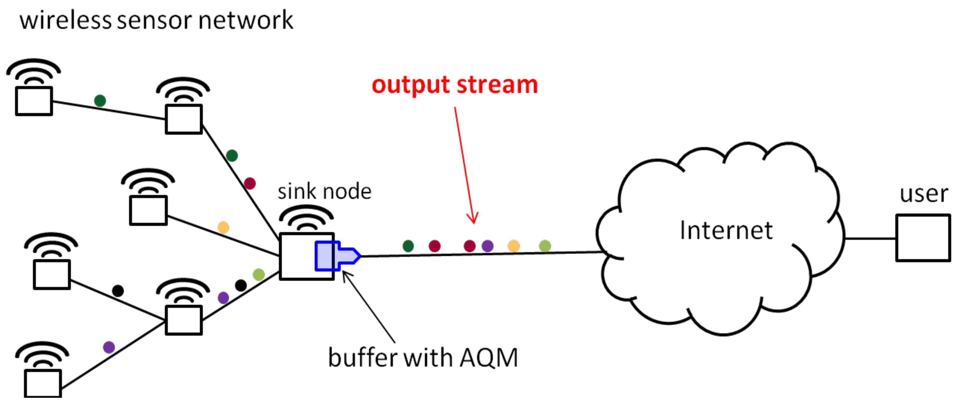
In this paper, we want to analyse the output stream from a buffer governed by this policy. A typical scenario is depicted in Figure 1. Specifically, we have a wireless sensor network of some topology and a sink node that collects data packets from sensor nodes. It transmits them further to a user through the internet (or to a local server first, but this is irrelevant here). Most importantly, the sink node has implemented an AQM mechanism at the buffer of its output interface (the blue part in Figure 1). Our interest lies in the statistical properties of the output stream from this buffer.
The buffer with AQM under study, in blue in Figure 1, is enlarged further in Figure 2. Namely, on the left-hand side of Figure 2, the traffic from the wireless sensor network, aggregated inside the sink node, is depicted. The packets from this traffic are subject to the AQM mechanism based on function . Specifically, every packet on arrival is subject to a random decision; it is dropped with probability , or it is deposited in the buffer of size N with probability . Argument k of function denotes the buffer occupancy at the time of each decision. The buffer in Figure 2 is meanwhile being drained by transmissions throughout the output link. Each packet transmission time is random and has an arbitrary distribution function . This distribution may account for variable packet sizes or a variable bitrate of the output link, or both. Lastly, the aggregated traffic, on the left-hand side of Figure 2, is modelled here by the BMAP process, whose powerful capabilities enable modelling of traffic of arbitrary type and complexity (this subject will be broadened later).
Note that the output stream on the right-hand side of Figure 2 must be essentially unlike the aggregated traffic on the left-hand side. First, this is because the AQM mechanism occasionally drops packets, which is its main goal for the reasons explained before. Therefore, even the output rate from the sink node is not equal to its input rate. Second, the transmission through the output link further changes the statistical properties of the output stream.
The purpose of this paper is to find the characteristics of the output stream in Figure 2 using instruments of queuing theory, and to study in numeric examples how the properties of the output stream vary with the properties of the model.
The paper proceeds with the following arrangements. In Section 2, the contribution of the paper is detailed. In Section 3, previous investigations in related fields are recalled. The model of the input stream, the packet buffer and its policy based on function are presented in Section 4. Then, in Section 5, a mathematical analysis of the output stream is conducted. In Section 6, numeric examples are shown and commented, with diverse parameterisations of the input stream, mechanism loads and functions . Lastly, the insights of this research work are summarised in Section 7. In the same section, suggestions for future work are provided.
2. Contribution
The primary contribution of this paper includes three new formulas: one for the average number of packets over time t in the output stream, one for the momentary packet output rate at time t and one for the steady-state output rate.
The secondary contribution of the paper is a set of numeric examples, exposing dependencies of the output stream characteristics on the model parameters. Specifically, five parameterisations of a BMAP are used in these examples, with different features of the input stream, and combined with different system loads and different forms of function to observe the impact of each on the output stream in both steady-state and time-dependent cases.
Why do the characteristics of the output stream matter?
From a networking standpoint, they matter because the considered output stream constitutes an input stream to another device. Specifically, the output stream in Figure 1 can be an input stream to a router, local or distant processing server, local or distant user, etc. Whatever the next device is, the performance of the whole system depends on the characteristics of the considered stream.
From a theoretical angle, the rate of the output stream is the key characteristic of the buffering mechanism, because it represents the overall performance of this mechanism, i.e., its ability to process a specific number of packets in a time unit.
Now, it is worth stressing that the results obtained here are broadly applicable in networks with completely different statistical properties of traffic and exploiting different functions . Such universality is a consequence of three assumptions on the analysed model.
Firstly, the batch Markovian arrival process (BMAP) is used to model the packet interarrival times in the aggregated traffic (see Figure 2). The BMAP has very powerful modelling capabilities—perhaps most powerful among all known point processes—which are analytically tractable. To name a few of these capabilities, the BMAP is able to model an arbitrary autocorrelation structure of the input stream, batch and single arrivals, and an arbitrary interarrival distribution [22,23]. It is known that all these features may influence the performance of the buffering policy. For instance, the effects of the interarrival distribution are known from elementary queueing theory [24]. The impact of the correlation structure was thoroughly investigated when positive autocorrelation was discovered in LANs [25]. The batch structure of traffic was shown to follow from the design of the TCP protocol [26], and is also known to deeply impact the queueing characteristics [24,27].
Secondly, the transmission times are assumed to have an arbitrary distribution. This means every needed packet length distribution can be used in numeric calculations.
3. Related Work
Based on the author’s knowledge, the results of this article are new.
Specifically, there are no published papers devoted to the output stream of packets leaving a buffer governed by the -based policy. This is rather unexpected, bearing in mind the importance of the -based policy in networking and the significance of the characteristics of the output stream, discussed in Section 2.
The work related to this paper can be categorised into four groups.
First, there are published articles on the output stream from a buffer for various types of input stream and = service time, but without the -based packet dropping policy. For instance, in the classic work [28], the output stream for a Poisson input stream and exponential service is shown to be Poisson. In [29], the case with a general, single, uncorrelated input stream and general service times is studied. In [30], a system with a batch, uncorrelated input stream and general service times is investigated. Lastly, some papers are devoted to analysis of the output stream from a buffer with correlated batch arrivals, see, e.g., [31,32,33].
In none of the mentioned above work was the -based dropping policy considered, whereas it is a crucial component of the system studied here. Obviously, this policy deeply influences the system performance in general and the output stream behaviour in particular.
Second, there are studies on buffers that do incorporate the -based policy, but without an analysis of the output stream. In these papers, different queueing characteristics are studied either via simulations [11,12,13,14,15,16,17] or mathematically [34,35,36,37,38,39,40,41,42] under diverse assumptions of system parameters. As it was argued above, the characteristics of the output stream are very important for both theoretical and practical reasons. Therefore, we study them herein.
Third, as it was already mentioned, there are papers on AQM, in which the probability of deletion of a packet at the buffer depends on different variables [1,4,5,6,7,8,9,10].
Fourth, there are many studies on the BMAP and queueing models for telecommunication networks, which are very loosely related to the model studied herein, see, e.g., [43,44,45,46] and the references provided there.
Lastly, it is worth mentioning that usage of the BMAP process is not limited to networking. Other real-world applications of the BMAP include inventory models [47,48], supply chain management [49], maintenance and spare parts [50], disaster models [51] and vehicular traffic [52,53].
All the mentioned references are gathered in Table 1, in which the originality of this paper is highlighted when compared to them.
4. Model
We are going to analyse the model depicted schematically in Figure 2.
To parametrise the BMAP, matrices , , are needed, each of size . They have to fulfill the following requirements:
- is negative on its diagonal but non-negative outside the diagonal;
- is non-negative for ;
- is a transition-rate matrix, i.e., each row of D sums to zero;
- .
Matrix D constitutes the intensity matrix of the underlying Markov chain of the BMAP, , which has possible states . In what follows, when saying that the BMAP is in state i, we will mean that this underlying chain is in state i, i.e., .
The evolution of governs arrivals of batches. In particular, diagonal entries of for correspond to arrivals of batches of length b, while off-diagonal entries correspond to arrivals of batches of length b together with changes in . Off-diagonal elements of correspond to changes in without arrivals. In practice, we usually deal with a few matrices only, each corresponding to a possible batch length. All the remaining values are zero.
Two important characteristics of a BMAP are and . Specifically, is the parameter of the exponentially distributed sojourn time before the next change of state, given that the BMAP is now in state i, whereas is the probability that after this sojourn time the state switches from i to j with arrival of a batch of b packets. It holds that
and
More on the mathematical properties of BMAPs can be found in the monograph [43].
Now, we presume that a buffer of capacity N packets is fed by a stream of packets modelled by a BMAP. The packets create an FIFO queue in this buffer, which is served from the head by a transmission process. The transmission time of each packet is random and distributed in accordance with some distribution function .
When N packets are present in the buffer, a newly incoming packet is deleted. However, even with fewer than N packets in the buffer, a new packet may be deleted. This may happen with every incoming packet with probability , where k denotes the buffer occupancy at the time of arrival of this new packet. Therefore, arguments of function are non-negative integers,
It is presumed that the packet being currently transmitted is the first one in the buffer; i.e., there is no separate room for the packet under service. Therefore, the phrase “buffer occupancy” includes the packet being transmitted, if any.
By we denote the rate of the aggregate input stream, i.e., the BMAP rate. The load of the buffering mechanism is:
where
is the average packet transmission time.
When characterising the output process, we will be interested in the following three characteristics: , and V.
Specifically, is the average number of packets occurring in the output stream in , assuming the buffer occupancy at was n and the state was i.
is the momentary rate of the output stream at time t, defined by:
Finally, V is the steady-state rate of the output stream, defined by:
All model parameters and characteristics of interest are gathered in Table 2.
Finally, note that herein we consider only the aggregated traffic without distinguishing between individual flows from users. The information about which packet comes from which individual user is not included in the BMAP. Naturally, the rates and distributions of particular users influence the aggregated traffic. Fortunately, several algorithms for fitting BMAP matrices to the aggregated traffic have already been proposed, see, for example, [22,23,55,56]. In these fitting algorithms, the rates and distributions of particular users are incorporated into the resulting BMAP matrices. We assume herein that we already have the BMAP matrices reflecting the statistical properties of the aggregated traffic and, indirectly, the particular users within it.
5. Output Stream Analysis
To make it easier to follow the derivations in this section, the workflow of the analysis of the output stream is shown in Figure 3.
Therefore, we begin derivations by constructing the first integral equation for .
Assume first that the buffer occupancy is 0 at . For an arbitrary initial state i, we have:
where and are given in (1) and (3), respectively. Furthermore, denotes the probability that on arrival of a batch of b packets, a packets are admitted to the buffer, while packets are dropped, presuming the buffer occupancy on the arrival of this batch is n. A formula for will be shown at the end of this section.
Equation (8) is inferred by conditioning on the initial moment of any change in the input stream, x. At time x, a packets are admitted to the buffer, so the new buffer occupancy is a, and the new state is j. There could not be any departure by x, so the new average number of packets departed by t, counting from x, will be .
Lastly, (13) can be ordered with regards to growing a as follows:
where
and I is the identity matrix.
Now, we can deal with the eventuality where the buffer occupancy is non-zero at . In such a situation, we can construct the following equation:
where denotes the probability that until the time x, the number of packets admitted to the buffer is a; the state at the time x is j, given that no departure took place by the time x; the initial occupancy was n; and the initial state was i.
Equation (17) is inferred by conditioning on a different moment to (8). Specifically, x in (17) is the first departure moment, distributed according to . Just after x, we have one packet already transmitted from the buffer, the new buffer occupancy of and the new state of j. Consequently, the new average number of packets departed by t, counting from x, will be .
Equations (14) and (23) constitute a system of algebraic equations with unknowns: . Combining these unknowns in a vertical vector , we can derive the solution of (14) and (23), which can be recapitulated as follows.
Theorem 1.
Take note that to use this result in practice, one needs to be able to calculate the values of functions and , which occur in (12) and (19), respectively. Both these functions are rather easy to compute recursively using the method shown in [40]. Specifically, for , we have:
and
which enables recursive calculation of for arbitrary n, b and a.
Note also that is, by definition, non-decreasing with respect to t. For a visualisation of the properties of the output stream, it is more convenient to use the time-dependent rate of the output stream, , which is defined in (6).
Applying the well-known derivative theorem on the Laplace transform, we have:
where
whereas can be calculated using (25).
The steady-state rate of the output stream, V, can be computed using another well-known property of the transform. Specifically, using the Final-Value Theorem on (40), we have:
with obtained from (25) again.
Lastly, note that (25) and (40) are expressed in the transform domain based on variable s. To return to the time domain, t, we have to employ an inversion method. A great variety of such methods is accessible (see monograph [57] on the subject). In the following numeric examples, the Zakian approach is exploited (Formula (7.12) in [57]).
6. Numeric Examples
In the numeric examples, we will use a few parameterisations of the BMAP which exemplify different features of the input stream. These include single arrivals, batch arrivals, positive autocorrelation, negative autocorrelation and no autocorrelation.
Specifically, the following five parameterisations will be employed:
- :
- :
- :
- :
- :
The total input rate of each of these streams is 1. and have single arrivals only, whereas – have batch arrivals. and are positively autocorrelated with a one-lag autocorrelation of 0.425, whereas and are negatively autocorrelated with a one-lag autocorrelation of −0.425. is not autocorrelated. Lastly, – have common average batch length of 5, and a common rate of arrivals of batches of 0.2.
Unless indicated otherwise, the following function will be utilised in the examples:
This is a negative-exponential function of REM type (see, e.g., [12]). The buffer on which this function operates is of length 32.
Unless indicated otherwise, the transmission time distribution is hyper-exponential with parameters , , , , the average value of 0.8 and the std. deviation of 0.94. Therefore, unless indicated otherwise, the system load is .
In Table 3, the rate of the output stream is shown for all considered BMAPs at different times and in the steady state, . In all instances, the buffer occupancy at was 0 and the initial state was 1.
Let us focus first on the steady-state output rate, shown in the last column of Table 3. As is evident, the rate may differ greatly depending on the internal nuances of the input stream. The worst result, 0.715, differs by almost 30% from the best result, 0.994, even though the input rate was the same in all cases. Note that 0.715 (or even 0.822) is a quite bad output rate, given that the system is significantly underloaded, .
Clearly, positive autocorrelation produces worse results than negative autocorrelation. Specifically, positively correlated produces a worse output rate than negatively correlated , while they both have no batch arrivals. Similarly, positively correlated provides a worse rate than negatively correlated , while they both have the same average batch length. It is interesting, however, that uncorrelated offers a slightly better rate than negatively correlated .
Moreover, batch arrivals produce worse results than single arrivals. This becomes evident if we compare with , and with . Within each of these pairs, the autocorrelation is common but the former input stream is single, whereas the latter is of batch type.
Summarising the steady-state results, the worst rate, 0.715, is obtained when both positive autocorrelation and the batch structure are involved, while the best rate, 0.994, is obtained when the autocorrelation is negative and there are no batch arrivals.
Now we can focus on the time-dependent output rates shown in Table 3. Apparently, the convergence time to the steady state may vary greatly depending on the internal nuances of the input stream. In the case of and , the steady-state output rate is achieved at the relatively low , whereas for , it is not achieved even at . The convergence time seems to be prolonged by positive autocorrelation and the batch structure. This can be observed by performing comparisons in the same pairs, as previously, i.e., vs. , vs. , vs. and vs. .
A detailed evolution in time of the output rate is depicted in Figure 4 and Figure 5 for all considered BMAPs. Figure 4 differs from Figure 5 in that the former is computed for an initially empty buffer, while the latter for an initially full buffer. In the full buffer scenario, the output rate is initially rather high for every considered BMAP. This is because efficient transmission () can temporarily provide an output rate greater than the input rate using packets stored in the buffer.
Interestingly, in both Figure 4 and Figure 5, the curves for and are close to each other, despite the fact that the former stream has no autocorrelation, whereas the latter has negative autocorrelation. Apparently, the negative autocorrelation provides very close (slightly worse) output rates to zero autocorrelation. Conversely, both these curves are in sharp contrast with the curve, obtained for positively autocorrelated input streams.
Lastly, we can observe in detail the convergence to the steady state in Figure 4 and Figure 5. For , and , each with negative or zero autocorrelation, the convergence is pretty quick. It is a little bit slower for , which has positive autocorrelation, but no batch arrivals, and much slower for , which has positive autocorrelation and batch arrivals.
A detailed evolution in time of the output rate, depending on the initial occupancy, is depicted in Figure 6 and Figure 7, for one selected input stream, . In both figures, the curves for initial occupancies of 0, 25%, 50%, 75% and 100% are shown. Figure 6 differs from Figure 7 in that the former is computed for the initial state 1, while the latter for the initial state of 3.
Firstly, we can notice that the initial state may severely influence the evolution of the output rate—the figures are not alike.
Secondly, the discussed above effect of the initially high output rate is not characteristic to the initially full buffer only. In fact, this effect occurs for every non-zero initial occupancy. Therefore, all the curves for differ greatly from the curve for in both Figure 6 and Figure 7.
In the next figure, we may examine the dependence of the steady-state output rate on the system load. To achieve that, parameters and of the transmission time distribution are scaled by a factor r, resulting in a variable system load from 0 to 2.
The results are depicted in Figure 8. For , which has neither a batch structure nor positive autocorrelation, a good output rate is maintained almost up to the load of 1. For , and , which have either batch arrivals or positive autocorrelation, the output rate begins to deteriorate much earlier, for the load about 0.6. However, the impact of the positive autocorrelation in prevails, and the output rate in this case drops faster than for and . Lastly, for , which has both a batch structure and positive autocorrelation, the output rate begins to deteriorate at as low a as 0.3. The shape of the curve is in this case quite close to the shape for —both curves were obtained for the same autocorrelation.
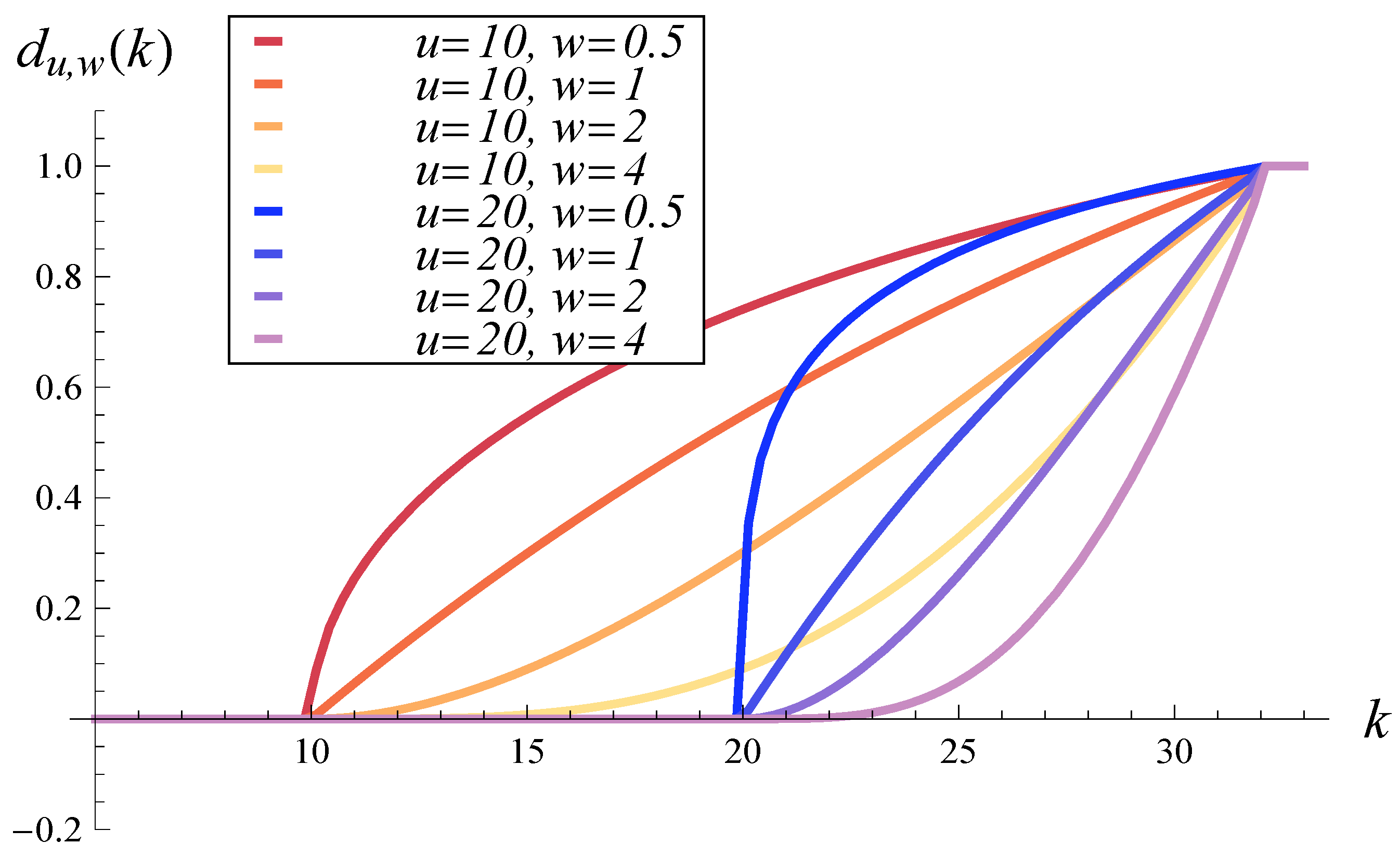
In the final set of results, we examine the dependence of the steady-state output rate on the function . To achieve this, we can focus on the most demanding input stream, , with a class of functions depending on two parameters, u and w:
where is given in (43).
Parameter u establishes the interval of effective operation of function , which is . Parameter w establishes how steep the function is, i.e., how quickly the dropping probability grows in the operation interval.
The resulting steady-state output rate as a function of u and w for is depicted in Figure 10. As one could foresee, the output rate grows with each of the two parameters. What is more interesting, however, is that both parameters seem to influence the output rate in a similar manner, i.e., the surface is almost symmetrical.
7. Conclusions
We analysed the output stream from a packet buffer governed by the policy that incoming packets are dropped with a probability related to the buffer occupancy.
In the mathematical part, formulas for the number of packets departing the buffer in a specific time, the time-dependent output rate and the steady-state output rate were derived. A powerful and versatile model of the input stream was used, the BMAP, and accompanied with a general transmission time distribution and a general function . These make the results broadly applicable in networks of completely different statistical properties of traffic and exploiting different probabilities.
In the numeric examples, we used the obtained formulas to examine the influence of the properties of the input stream, system load and function on the properties of the output stream.
7.1. Insights of this Research Work
In the steady-state examples, it was shown that the output rate may differ greatly depending on the internal nuances of the input stream, even if the input rate is unaltered. Furthermore, it was demonstrated that the output rate can be quite low, even if the load of the buffering mechanism is low.
An essential takeaway from this is the following. For a given input packet rate , a given load and a particular function , there is absolutely nothing we can say about the output rate without taking into consideration the internal statistical structure of the input stream.
As was demonstrated, the most important factors causing deterioration of the output rate are the batch structure and positive autocorrelation, especially when combined together. Interestingly, a negative correlation in the input stream produced a slightly worse output rate than a zero correlation.
In the time-dependent examples, its was shown that a batch structure and positive autocorrelation make the convergence time to the steady state much longer than in the case without these factors.
Lastly, it was established that a batch structure and positive autocorrelation can cause much quicker deterioration of the output rate with a growing load.
Namely, in uncorrelated examples with single arrivals, close to the maximum output rate was maintained up to the load approaching 1. If either batch arrivals or positive correlation was introduced, the output rate started to deteriorate at the load of about 0.6. If, however, both these factors were combined together, the output rate began to deteriorate at as low a load as 0.3.
7.2. Future Work
Future work can branch off in several ways.
First, the buffering mechanism from Figure 2 can be further studied with respect to other characteristics. For example, the average response time of this mechanism has not been derived so far. The response time of a system is the total time that a packet spends in this system. (Herein, it would be the time spent in the buffer plus the transmission time.) It is therefore a key characteristic of the mechanism, reflecting the latency that it adds to the entire packet delivery time.
Second, extensions of the mechanism in Figure 2 can be proposed and studied. For example, instead of one function , a separate function for each flow of traffic can be used. For some reasons, we may prefer to filter one flow differently than another.
Third, completely different AQM mechanisms than those considered here can be analysed using queueing models, e.g., the mechanisms of [1,4,5,6,7,8,9,10]. To date, they have been tested mainly using network simulations.
Finally, computations for other transmission time distributions can be carried out, e.g, gamma, uniform, degenerate, etc., distributions.
Funding
This research received no external funding.
Data Availability Statement
Data is contained within the article.
Conflicts of Interest
The author declares no conflict of interest.
References
- Nichols, K.; Jacobson, V. Controlling Queue Delay. Queue 2012, 55, 42–50. [Google Scholar]
- Internet Engineering Task Force. Request for Comments 7567: ETF Recommendations Regarding Active Queue Management; Baker, F., Fairhurst, G., Eds.; 2015; Available online: https://datatracker.ietf.org/doc/rfc7567/ (accessed on 12 November 2023).
- Internet Engineering Task Force. Request for Comments 7928: Characterization Guidelines for Active Queue Management (AQM); Kuhn, N., Natarajan, P., Khademi, N., Eds.; 2016; Available online: https://datatracker.ietf.org/doc/html/rfc7928 (accessed on 12 November 2023).
- Pan, R.; Natarajan, P.; Piglione, C.; Prabhu, M.S.; Subramanian, V.; Baker, F.; VerSteeg, B. PIE: A lightweight control scheme to address the bufferbloat problem. In Proceedings of the IEEE International Conference on High Performance Switching and Routing, Taipei, Taiwan, 8–11 July 2013; pp. 148–155. [Google Scholar]
- Kahe, G.; Jahangir, A.H. A self-tuning controller for queuing delay regulation in TCP/AQM networks. Telecommun. Syst. 2019, 71, 215–229. [Google Scholar] [CrossRef]
- Belamfedel Alaoui, S.; Tissir, E.H.; Chaibi, N. Analysis and design of robust guaranteed cost Active Queue Management. Comput. Commun. 2020, 159, 124–1321. [Google Scholar] [CrossRef]
- Wang, H. Trade-off queuing delay and link utilization for solving bufferbloat. ICT Express 2020, 6, 269–272. [Google Scholar] [CrossRef]
- Hotchi, R.; Chibana, H.; Iwai, T.; Kubo, R. Active queue management supporting TCP flows using disturbance observer and Smith predictor. IEEE Access 2020, 8, 173401–173413. [Google Scholar] [CrossRef]
- Wang, C.; Chen, X.; Cao, J.; Qiu, J.; Liu, Y.; Luo, Y. Neural Network-Based Distributed Adaptive Pre-Assigned Finite-Time Consensus of Multiple TCP/AQM Networks. IEEE Trans. Circuits Syst. 2021, 68, 387–395. [Google Scholar] [CrossRef]
- Shen, J.; Jing, Y.; Ren, T. Adaptive finite time congestion tracking control for TCP/AQM system with input saturation. Int. J. Syst. Sci. 2022, 53, 253–264. [Google Scholar] [CrossRef]
- Floyd, S.; Jacobson, V. Random early detection gateways for congestion avoidance. IEEE ACM Trans. Netw. 1993, 1, 397–413. [Google Scholar] [CrossRef]
- Athuraliya, S.; Li, V.H.; Low, S.H.; Yin, Q. REM: Active queue management. IEEE Netw. 2001, 15, 48–53. [Google Scholar] [CrossRef]
- Zhou, K.; Yeung, K.L.; Li, V. Nonlinear RED: Asimple yet efficient active queue management scheme. Comput. Netw. 2006, 50, 3784. [Google Scholar] [CrossRef]
- Domanska, J.; Augustyn, D.; Domanski, A. The choice of optimal 3-rd order polynomial packet dropping function for NLRED in the presence of self-similar traffic. Bull. Pol. Acad. Sci. Tech. Sci. 2012, 60, 779–786. [Google Scholar] [CrossRef]
- Gimenez, A.; Murcia, M.A.; Amigó, J.M.; Martínez-Bonastre, O.; Valero, J. New RED-Type TCP-AQM Algorithms Based on Beta Distribution Drop Functions. Appl. Sci. 2022, 12, 11176. [Google Scholar] [CrossRef]
- Feng, C.; Huang, L.; Xu, C.; Chang, Y. Congestion Control Scheme Performance Analysis Based on Nonlinear RED. IEEE Syst. J. 2017, 11, 2247–2254. [Google Scholar] [CrossRef]
- Patel, S.; Karmeshu. A New Modified Dropping Function for Congested AQM Networks. Wirel. Pers. Commun. 2019, 104, 37–55. [Google Scholar] [CrossRef]
- Zhao, S.; Wang, P.; He, J. Simulation analysis of congestion control in WSN based on AQM. In Proceedings of the 2011 International Conference on Mechatronic Science, Electric Engineering and Computer (MEC), Jilin, China, 19–22 August 2011; pp. 197–200. [Google Scholar]
- Ghaffari, A. Congestion control mechanisms in Wireless Sensor Networks: A survey. J. Netw. Comput. Appl. 2015, 52, 101–115. [Google Scholar] [CrossRef]
- Asonye, E.A.; Musa, S.M. Analysis of Personal Area Networks for ZigBee Environment Using Random Early Detection-Active Queue Management Model. In Proceedings of the International Conference on Industrial Engineering and Operations Management, Toronto, ON, Canada, 23–25 October 2019; pp. 1441–1455. [Google Scholar]
- Kumar, H.; Kumar, S.M.D.; Nagarjun, E. Congestion Estimation and Mitigation Using Fuzzy System in Wireless Sensor Network. Lect. Notes Netw. Syst. 2022, 329, 655–667. [Google Scholar]
- Klemm, A.; Lindemann, C.; Lohmann, M. Modeling IP traffic using the batch Markovian arrival process. Perform. Eval. 2003, 54, 149–173. [Google Scholar] [CrossRef]
- Salvador, P.; Pacheco, A.; Valadas, R. Modeling IP traffic: Joint characterization of packet arrivals and packet sizes using BMAPs. Comput. Netw. 2004, 44, 335–352. [Google Scholar] [CrossRef]
- Cohen, J.W. The Single Server Queue, Revised ed.; North-Holland Publishing Company: Amsterdam, The Netherlands, 1982. [Google Scholar]
- Lel, W.; Taqqu, M.; Willinger, W.; Wilson, D. On the self-similar nature of ethernet traffic (extended version). IEEE/ACM Trans. Netw. 1994, 2, 1–15. [Google Scholar]
- Garetto, M.; Towsley, D. An efficient technique to analyze the impact of bursty TCP traffic in wide-area networks. Perform. Eval. 2008, 65, 181–202. [Google Scholar] [CrossRef]
- Chydzinski, A.; Samociuk, D.; Adamczyk, B. Burst ratio in the finite-buffer queue with batch Poisson arrivals. Appl. Math. Comput. 2018, 330, 225–238. [Google Scholar] [CrossRef]
- Burke, P.J. The output of a queueing system. Oper. Res. 1956, 4, 699–704. [Google Scholar] [CrossRef]
- Girish, M.K.; Hu, J.-Q. Approximations for the departure process of the G/G/1 queue with Markov-modulated arrivals. Eur. J. Oper. Res. 2001, 134, 540–556. [Google Scholar] [CrossRef]
- Kempa, W.M. The departure process for queueing systems with batch arrival of customers. Stoch. Model. 2008, 24, 246–263. [Google Scholar] [CrossRef]
- Ferng, H.-W.; Chang, J.-F. Departure processes of BMAP/G/1 queues. Queueing Syst. 2001, 39, 109–135. [Google Scholar] [CrossRef]
- Zhang, Q.; Heindl, A.; Smirni, E. Models of the departure process of a BMAP/MAP/1 queue. Perform. Eval. Rev. 2005, 33, 18–20. [Google Scholar] [CrossRef]
- Zhang, Q.; Heindl, A.; Smirni, E. Characterizing the BMAP/MAP/1 departure process via the ETAQA truncation. Stoch. Model. 2005, 21, 821–846. [Google Scholar] [CrossRef]
- Hao, W.; Wei, Y. An Extended GIX/M/1/N Queueing Model for Evaluating the Performance of AQM Algorithms with Aggregate Traffic. Lect. Notes Comput. Sci. 2005, 3619, 395–414. [Google Scholar]
- Kempa, W.M. Time-dependent queue-size distribution in the finite GI/M/1 model with AQM-type dropping. Acta Electrotech. Inform. 2013, 13, 85–90. [Google Scholar] [CrossRef]
- Kempa, W.M. A direct approach to transient queue-size distribution in a finite-buffer queue with AQM. Appl. Math. Inf. Sci. 2013, 7, 909–915. [Google Scholar] [CrossRef]
- Tikhonenko, O.; Kempa, W.M. Performance evaluation of an M/G/N-type queue with bounded capacity and packet dropping. Appl. Math. Comput. Sci. 2016, 26, 841–854. [Google Scholar] [CrossRef]
- Tikhonenko, O.; Kempa, W.M. Erlang service system with limited memory space under control of AQM mechanizm. Commun. Comput. Inf. Sci. 2017, 718, 366–379. [Google Scholar]
- Chydzinski, A.; Barczyk, M.; Samociuk, D. The Single-Server Queue with the Dropping Function and Infinite Buffer. Math. Probl. Eng. 2018, 2018, 3260428. [Google Scholar] [CrossRef]
- Chydzinski, A.; Mrozowski, P. Queues with dropping functions and general arrival processes. PLoS ONE 2016, 11, e0150702. [Google Scholar] [CrossRef] [PubMed]
- Chydzinski, A. Non-Stationary Characteristics of AQM Based on the Queue Length. Sensors 2023, 23, 485. [Google Scholar] [CrossRef] [PubMed]
- Chydzinski, A. Loss Process at an AQM Buffer. J. Sens. Actuator Netw. 2023, 12, 55. [Google Scholar] [CrossRef]
- Dudin, A.N.; Klimenok, V.I.; Vishnevsky, V.M. The Theory of Queuing Systems with Correlated Flows; Springer: Cham, Switzerland, 2020. [Google Scholar]
- Vishnevskii, V.M.; Dudin, A.N. Queueing systems with correlated arrival flows and their applications to modeling telecommunication networks. Autom. Remote Control 2017, 78, 1361–1403. [Google Scholar] [CrossRef]
- Baek, J.W.; Lee, H.W.; Lee, S.W.; Ahn, S. A workload factorization for BMAP/G/1 vacation queues under variable service speed. Oper. Res. Lett. 2014, 42, 58–63. [Google Scholar] [CrossRef]
- Banik, A.D.; Chaudhry, M.L.; Wittevrongel, S.; Bruneel, H. A simple and efficient computing procedure of the stationary system-length distributions for GIX/D/c and BMAP/D/c queues. Comput. Oper. Res. 2022, 138, 105564. [Google Scholar] [CrossRef]
- Dudin, A.; Klimenok, V. Analysis of MAP/G/1 queue with inventory as the model of the node of wireless sensor network with energy harvesting. Ann. Oper. Res. 2023, 331, 839–866. [Google Scholar] [CrossRef]
- Krishnamoorthy, A.; Joshua, A.N.; Kozyrev, D. Analysis of a Batch Arrival, Batch Service Queuing-Inventory System with Processing of Inventory While on Vacation. Mathematics 2021, 9, 419. [Google Scholar] [CrossRef]
- Barron, Y. A threshold policy in a Markov-modulated production system with server vacation: The case of continuous and batch supplies. Adv. Appl. Probab. 2018, 50, 1246–1274. [Google Scholar] [CrossRef]
- Baek, J.W.; Lee, H.W.; Lee, S.W.; Ahn, S. A MAP-modulated fluid flow model with multiple vacations. Ann. Oper. Res. 2013, 202, 19–34. [Google Scholar] [CrossRef]
- Dudin, A.; Karolik, A. BMAP/SM/1 queue with Markovian input of disasters and non-instantaneous recovery. Perform. Eval. 2001, 45, 19–32. [Google Scholar] [CrossRef]
- Alfa, A.S. Modelling traffic queues at a signalized intersection with vehicle-actuated control and Markovian arrival processes. Comput. Math. Appl. 1995, 30, 105. [Google Scholar] [CrossRef]
- Alfa, A.S.; Neuts, M.F. Modelling vehicular traffic using the discrete time Markovian arrival process. Transp. Sci. 1995, 29, 109–117. [Google Scholar] [CrossRef]
- Lucantoni, D.M. New results on the single server queue with a batch Markovian arrival process. Commun. Stat. Stoch. Model. 1991, 7, 1–46. [Google Scholar] [CrossRef]
- Breuer, L. An EM algorithm for batch Markovian arrival processes and its comparison to a simpler estimation procedure. Ann. Oper. Res. 2002, 112, 123–138. [Google Scholar] [CrossRef]
- Casale, G.; Zhang, E.Z.; Smirni, E. Trace data characterization and fitting for Markov modeling. Perform. Eval. 2010, 67, 61–79. [Google Scholar] [CrossRef]
- Cohen, A.M. Numerical Methods for Laplace Transform Inversion; Springer: New York, NY, USA, 2007. [Google Scholar]
Figure 1.
An output stream from a wireless sensor network through a buffer with AQM.

Figure 2.
Buffer with AQM from Figure 1 in detail.
Figure 2.
Buffer with AQM from Figure 1 in detail.

Figure 3.
Workflow of derivations.

Figure 4.
Time-dependent rate of the output stream for different input streams. , .

Figure 5.
Time-dependent rate of the output stream for different input streams. , .

Figure 6.
Time-dependent rate of the output stream for and different initial buffer occupancies. .

Figure 7.
Time-dependent rate of the output stream for and different initial buffer occupancies. .

Figure 8.
Steady-state rate of the output stream versus load for different input streams.

Figure 9.
Function for different combinations of parameters u and w.

Figure 10.
Steady-state rate of the output stream for vs. parameters u and w in .


Table 1.
Research related to AQM, the BMAP and the output stream.
| -based AQM, | this work |
| analysis of the output stream | |
| no AQM at all, | [28,29,30,31,32,33] |
| analysis of the output stream | |
| -based AQM, | [11,12,13,14,15,16,17,34,35,36,37,38,39,40,41,42] |
| no analysis of the output stream | |
| different AQM to here, | [1,4,5,6,7,8,9,10] |
| various characteristics | |
| BMAP traffic models and queueing, | a vast literature, see [43,44,45,46,47,48,49,50,51,52,53] |
| no AQM at all | and the references there |
Table 2.
Summary of model parameters and characteristics of interest.
| BMAP matrices (parameters of the input stream) | |
| underlying Markov chain of the BMAP | |
| N | buffer size in packets |
| dropping probability for buffer occupancy k in AQM | |
| distribution function of the packet transmission time | |
| M | number of states of |
| packet input rate | |
| load of the buffering mechanism | |
| average packet transmission time | |
| V | state-state rate of the output stream |
Table 3.
Rate of the output stream at different times for different input streams. , .
| 0.536 | 0.717 | 0.809 | 0.822 | 0.822 | 0.822 | |
| 0.941 | 0.980 | 0.994 | 0.994 | 0.994 | 0.994 | |
| 0.830 | 0.900 | 0.908 | 0.908 | 0.908 | 0.908 | |
| 0.351 | 0.434 | 0.526 | 0.627 | 0.710 | 0.715 | |
| 0.801 | 0.886 | 0.893 | 0.894 | 0.894 | 0.894 |
Disclaimer/Publisher’s Note: The statements, opinions and data contained in all publications are solely those of the individual author(s) and contributor(s) and not of MDPI and/or the editor(s). MDPI and/or the editor(s) disclaim responsibility for any injury to people or property resulting from any ideas, methods, instructions or products referred to in the content. |
© 2024 by the author. Licensee MDPI, Basel, Switzerland. This article is an open access article distributed under the terms and conditions of the Creative Commons Attribution (CC BY) license (https://creativecommons.org/licenses/by/4.0/).
Share and Cite
MDPI and ACS Style
Chydzinski, A. Output Stream from the AQM Queue with BMAP Arrivals. J. Sens. Actuator Netw. 2024, 13, 4. https://doi.org/10.3390/jsan13010004
AMA Style
Chydzinski A. Output Stream from the AQM Queue with BMAP Arrivals. Journal of Sensor and Actuator Networks. 2024; 13(1):4. https://doi.org/10.3390/jsan13010004
Chicago/Turabian StyleChydzinski, Andrzej. 2024. "Output Stream from the AQM Queue with BMAP Arrivals" Journal of Sensor and Actuator Networks 13, no. 1: 4. https://doi.org/10.3390/jsan13010004
Note that from the first issue of 2016, this journal uses article numbers instead of page numbers. See further details here.