
Dynamic Boundary Optimization of Free Route Airspace Sectors


College of Civil Aviation, Nanjing University of Aeronautics and Astronautics, No. 29 Jiangjun Avenue, Nanjing 211106, China
*
Author to whom correspondence should be addressed.
Aerospace 2022, 9(12), 832; https://doi.org/10.3390/aerospace9120832
Submission received: 14 November 2022
/
Revised: 6 December 2022
/
Accepted: 13 December 2022
/
Published: 15 December 2022
(This article belongs to the Collection Air Transportation—Operations and Management)
Abstract
:Free Route Airspace (FRA) permits users to freely plan routes between defined entry and exit waypoints with the possibility of routing via intermediate waypoints, which is beneficial to improve flight efficiency. Dynamic management of sectors is essential for the future promotion of full-time FRA applications. In this paper, considering the demand uncertainty at the pre-tactical level, we construct an FRA complexity indicator system and use the XGBoost algorithm to predict the ATC workload. A two-stage sector boundary optimization method is proposed, using Binary Space Partition (BSP) to generate sector boundaries and an A*-based heuristic algorithm to automatically tune them to conform to the operational structure and “direct to” characteristics of FRA. Finally, this paper verifies the effectiveness of the proposed method for balancing ATC workload in a pre-designed Lanzhou FRA in China.
1. Introduction
In response to the increasing air traffic delays and the need for new Air Traffic Management (ATM) solutions, The Single European Sky ATM Research (SESAR) project was established in 2008. The SESAR program introduces the User Preferred Routing (UPR) or free routing concept to enable airspace users to plan freely 4D trajectories that suit them best [1].
EUROCONTROL subsequently initiated the coordinated development and implementation of Free Route Airspace (FRA). In FRA, users freely plan a route between the defined entry and exit fixes, with the possibility of routing via intermediate points [2]. According to EUROCONTROL [3], more than three-quarters of Europe’s airspace has now been implemented with FRA. When FRA is fully implemented, airspace users could save 1 billion nautical miles, 6 million tons of fuel consumption, 20 million tons of CO2 emissions, and 5 billion euros in fuel costs compared to the current situation.
Currently, FRA is mostly used in off-peak hours. As the traffic demand continues to grow, the problem of balancing FRA capacity and traffic demand becomes more complex. In order to adapt to the high-density traffic demand in the future full-time applications of FRA, one solution is the Dynamic Airspace Configuration (DAC) from the supply-side. DAC does not rely on fixed geographic features such as fixes, airways, and sectors but allocates airspace as a resource to meet user demand while also addressing weather, safety, security, and environmental constraints [4].
Most of the current research literature on DAC is applied to fixed-route airspace, and the main methods include discrete airspace, Voronoi diagram, dynamic airspace block, weighted graph model, etc. The research on DAC methods in FRA is still rarely reported. In addition, many of the current research methods of DAC have problems such as rough sector boundaries that require manual adjustment and costly reconfiguration of sectors at high frequencies. This paper introduces an efficient and automatic DAC method applied to FRA to dynamically optimize the sector boundaries to alleviate the capacity–demand imbalance. The main contribution of this paper is two-fold. One is that we empirically measure the demand uncertainty level in terms of complexity indicators, which are used to improve the reliability of the complexity-based workload prediction model at the pre-tactical phase. The other is that we propose a two-stage dynamic optimization method of sector boundary adjustment, especially an A*-based heuristic algorithm that automatically tunes the boundaries to conform to the operational structure and “direct to” characteristics of the FRA. The achievements of this paper contribute to refining the methodological framework of dynamic airspace management for full-time FRA applications.
The rest of this paper is organized as follows. Section 2 introduces the related work on DAC in recent years. In Section 3, we first establish a data-driven ATC workload prediction model based on an elected Complexity Indicator System (CIS) considering operational uncertainty using the XGBoost algorithm. Then a two-stage sector boundary optimization and automatic fine-tuning method is proposed. In Section 4, the effectiveness of the proposed method for balancing the ATC workload is verified in a pre-designed Lanzhou FRA in China. Finally, some conclusions are provided in Section 5.
2. Related Work
Worldwide, scholars have conducted numerous research on DAC problems in recent years. Most of them are applied to fixed-route airspace, which are absolutely worth learning for FRA management.
DAC has three main objectives: minimizing ATC workload, minimizing the variation in workload between ATCos, and minimizing the variation between successive configurations [5]. For the ATC workload, we can use air traffic complexity to assess it [6]. Air traffic complexity can characterize traffic posture. For example, the authors of [7] used deep convolutional neural networks to evaluate airspace operation complexity using air traffic as images; Kudumija et al. [8] used fast time simulations with the Performance Review Unit (PRU) complexity model to observe how air traffic complexity was affected through FRA implementation; Cao et al. [9] proposed a new sector operation complexity evaluation framework based on knowledge transfer specifically for the small-training-sample environment; the authors of [10] presented a new air traffic complexity metric based on linear dynamical systems, of which the goal is to quantify the intrinsic complexity of a set of aircraft trajectories.; and Isufaj et al. [11] introduced the concept of single aircraft complexity to determine the contribution of each aircraft to the overall complexity of air traffic. In terms of traffic complexity forecasting ATC workload, Manning et al. [12] compared the relative effectiveness of sector activity and sector complexity in predicting ATC task load; Gianazza et al. [13,14] used a neural network to provide ATCs with workload indications through the input of complexity metrics and explored all combinations of basic airspace modules using a tree search approach to construct the best airspace partition with the most balanced workload possible; Loft et al. [15] reviewed studies in which traffic factors, airspace factors, and operational constraints effectively predict ATC workload; and Marr et al. [16] used the Monitor Alert Parameter (MAP) instead of the workload metric to estimate based on traffic volume and complexity.
There are four main methods of DAC [5]: region-based DAC, graph-based DAC, trajectory-based DAC, and hybrid methods.
Region-based DAC mainly decomposes the airspace into small polygonal cells and uses clustering algorithms to cluster these cells to form sectors. For example, Refs. [17,18] discretized the airspace into hexagonal grids and clustered the grid cells to form new sector assignments using integer programming and knapsack algorithms; Refs. [19,20] discretized the airspace into rectangular grids and modeled the air traffic configuration using mathematical models such as Markov chains and vehicle-routing; Ref. [21] divided the airspace into small volume units and used metaheuristics to solve the resulting fuzzy dynamic airspace sectorization problem; and Wei et al. [22,23,24] discretized the terminal area airspace and solved the optimal sector division scheme based on algorithms such as constrained k-means clustering algorithm, integer programming techniques, and alpha shapes based sectorization algorithm, which can effectively reduce the complexity of traffic flow and make the sector division well adapted to the changes of traffic flow.
Graph-based DAC divides the airspace into multiple subgraphs. Usually, the partition is stopped after the expected number of subgraphs and a relatively balanced workload of subgraphs are obtained. For example, [25] used the Dynamic Airspace Unit Slices (DAU Slices) method to assign airspace slicing units according to real-time traffic flow assignment requirements; Ref. [26] used Voronoi diagrams and genetic algorithms to give different sector allocation schemes based on airspace sectors changing every two hours; Yousefi et al. [27] used a mixed integer planning algorithm and Binary Space Partition (BSP) method effectively equalized the aircraft dwell time and sector assignment over a large area, but the sector boundaries were coarse and needed to be adjusted manually; BASU et al. [28] used the BSP algorithm to implement sectorization in North America; Tang et al. [29] compared the advantages and disadvantages of KD-Tree, Bisection, and Voronoi Diagrams. In addition to the above methods, many scholars have used Weighted Graph Model (WGM) to model the airspace to facilitate DAC studies. The WGM uses waypoints and airports as vertices, route segments as links, and attaches weights to the links according to the air traffic volume. In [30,31], after establishing the WGM, a spectral clustering algorithm is used to form airspace zones, and then the zones are input to sectorize the entire airspace using the shortest path search algorithm and Dijkstra’s algorithm; Discrete Particle Swarm Optimization algorithm [32], NSGA-II algorithm [33], and genetic algorithm [34] are also used to perform WGM to generate new sectors.
Trajectory-based DAC prioritizes the formation of sector boundaries around the user’s preferred route while dynamically balancing the traffic density of each area. For example, [35,36] clustered flight trajectories with the innovation of balancing the dynamic density of aircraft for airspace zoning; Xu et al. [30] used a collaborative Air Traffic Flow Management (ATFM) strategy approach to incorporate traffic control initiatives and airspace dynamic opening schemes into a centralized optimization model that achieves simultaneous demand and capacity balancing by optimizing traffic flow and airspace configurations; and Lucic et al. [37] developed a template-based approach for the interaction of DAC and Traffic Flow Management (TFM) that allows demand and capacity balancing optimization in the presence of weather-related events or other uncertainties.
Hybrid approaches mix two and more of the above or other DAC methods, e.g., [38] created a network flow graph and discretized the airspace into rectangular grids, and partitioned the sectors by assigning grid cells to network flow graph nodes; Gerdes et al. [39,40,41] combined traffic flow fuzzy clustering, Voronoi diagrams, and evolutionary algorithm to propose a new method for dynamic airspace partitioning based on controller task load; and Chen et al. [42] used a combination of General Weighted Graph Cuts Algorithm, Optimal Dynamic Load Balancing Algorithm and heuristic KL algorithm hybrid algorithm to partition the sectors for a given null domain.
For the DAC approach in FRA, Lema-Esposto et al. [43] set up airspace building blocks and used a single-layer State-Task Network (STN) to model the configuration of airspace blocks that can efficiently dynamically allocate airspace capacity according to traffic demand and complexity; Sergeeva et al. [44,45] used an artificial evolution-based stochastic optimization algorithm and genetic algorithm to achieve dynamic sector delineation based on WGM; in Flight Centric Air Traffic Control (FCA), Gerdes et al. [40,41] clustered traffic flows and combined Voronoi diagrams and evolutionary algorithms to optimize the airspace to provide an appropriate airspace structure for future 4D flight trajectories.
It can be found that the sector boundaries generated by some DAC methods are coarse. For example, Yousefi et al. [17] took the middle point of each hexagonal cell and formed the sector boundaries along the gap between the points; the sector boundaries generated by literature [19,22,23,24] are all distributed along the grid cell boundaries and lack smoothness; Yousefi et al. [27] used mixed integer programming and BSP to generate sector boundaries that required further manual adjustments. The authors of [30,31] used the shortest path search algorithm and Dijkstra’s algorithm to generate the sector boundaries, but the process of generating path points is relatively complex.
In this paper, we perform ATC workload prediction based on traffic complexity indicators with the consideration of uncertainty and use a graph-based DAC method for the dynamic optimization of sector boundaries. Moreover, we propose an improved sector boundary optimization algorithm based on the A* algorithm, using the internal waypoints of FRA and known entry/exit points to optimize and modify the sector boundary generated by BSP, so that the new sector generated is more reasonable and convenient for “direct-to” operations of FRA.
3. Methods
3.1. ATC Workload Estimation Model in FRA
In this section, the Complexity Indicator System (CIS) of FRA is first constructed, and each sector’s complexity indicators are measured per unit time. To improve the efficiency and reliability of ATC workload estimation, the uncertainty analysis of complexity indicators is performed based on the variation of the complexity indicators, and the Extreme Gradient Boosting (XGBoost) is used to derive the magnitude of complexity indicators’ influence on workload estimation. The complexity indicators with lower uncertainty and more substantial influence are selected to build the ATC workload estimation model in FRA, which lays the foundation for subsequent sector boundary dynamic optimization. It is noted that only the command controller’s (similar to the executive Controller in Europe) workload is considered according to the specific organization of the ATC team in China [46].
3.1.1. CIS and Its Uncertainty Analysis
Based on the existing research literature on complexity indicators [9,47,48,49,50,51] and combined with the FRA characteristics, we selected the following 11 indicators to establish the CIS as shown in Table 1.
There are deviations in trajectories from flight plans due to traffic management, weather, control command, etc. To measure the uncertainty of trajectories under similar flight plans, we analyze the uncertainty of the above complexity indicators in the airspace sectors. Assuming that the flight plans of the same day of the week are similar, we calculate the complexity indicators of airspace sectors in the same time slices of different days based on the basic data of the airspace sectors and the historical flight trajectory.
The value of the statistical sector complexity indicator in the time slice on the statistical day is . To eliminate the influence of the dimension on the uncertainty of the complexity indicator, the values of indicators are normalized, so that the numerical range of different complexity indicators is within the interval , while remaining in the same distribution as the original data:
where is the maximum value of the indicator , and is the minimum value of the indicator .
Based on the normalized value of airspace complexity indicators, the standard deviation of the distribution is used to measure the variation of the indicator in each time slice during the statistical period days:
where is the average value of indicator in the time slice .
The average value of the standard deviation of each complexity indicator over all time slices (containing both peak and off-peak traffic time frame) is calculated to measure the uncertainty of the indicator :
where is the number of time slices, in this paper one time slice is 1 h, which means n = 24.
Based on the statistical results of the complexity indicators of each sector, the corresponding uncertainty values of the complexity indicators are calculated. The results of complexity indicator uncertainty calculation for different airspace sectors are used as features to cluster complexity indicators using the K-Means clustering algorithm to determine high, medium, and low uncertainty indicators.
3.1.2. XGBoost-Based Workload Estimation Model Using CIS
The data source for workload prediction is generated by the AirTOp simulator, which uses an event-based load generation method to calculate the ATC workload. It is important that before conducting the simulation, the baseline model, especially the event-based workload parameters shall be firstly calibrated and validated. In order to improve the accuracy of workload simulation, we invited the air traffic controllers from Lanzhou ATC center to calibrate the parameters for each event collected by the simulator. After the iterated “parameter adjustment-simulation-comparison-parameter adjustment” process, the simulated workload and traffic situation finally converged to the actual ones. Then, reliable workload training set based on random flight plans are generated by the well-calibrated FRA simulation scenarios using the AirTOp.
The XGBoost (Extreme Gradient Boosting) is a popular supervised learning algorithm based on decision trees [52]. The XGBoost-based workload estimation process for FRA sectors is as follows:
- (a)
- Calculation and standardization of the indicators in the CIS based on flight plan data;
- (b)
- Use XGBoost model to derive high impact indicators;
- (c)
- Combine low uncertainty indicators to generate a sample set and divide the sample set into training sample set and test sample set;
- (d)
- Inputting the training sample set into the XGBoost model and adjusting the parameters to meet the accuracy requirements;
- (e)
- Import the sample data of the sectors to be measured into the model, and derive the prediction results.
The flowchart of XGBoost-based workload estimation for FRA sectors is shown in Figure 1.
3.2. Dynamic Boundary Optimization Model of FRA Sectors
3.2.1. Objective Function
The ATC workload of each sector in the airspace should be balanced as much as possible to ensure the maximum utilization of airspace resources [53]. Therefore, the primary objective of dynamic boundary optimization is to balance the workload of each sector. For simplification, we assume that the subjective characteristics (e.g., acceptable workload threshold) of air traffic controllers are homogeneous. The objective function should be:
where is the ATC workload for the th sector, is the average ATC workload of all sectors, is the number of sectors, is the degree of balance of workload.
In addition, it is necessary to try to ensure that the sector coordination load in the airspace is minimized, i.e., the number of aircraft crossing the sector boundaries is minimized at time [54].
3.2.2. Constraints
In the process of sector boundary optimization, the influence of the route structure, sector shape, and restricted area on the geometric boundary of the sector needs to be considered to ensure the flight safety of aircraft and reduce the difficulty of sector control.
In this paper, sector boundary optimization is required to satisfy the following constraints [55]:
- (a)
- Convex constraint of the sector
Aircraft should avoid crossing the same sector two or more times during a flight. Convex constraints can ensure that aircraft do not repeatedly enter and exit the sector leading to increased sector coordination handover load. Concave boundaries are not unacceptable for all cases, as long as the sector boundary optimization does not cause traffic flow to enter the same sector twice or more.
Let the sequence of vertices of the sector be counterclockwise () and the th boundary be ; indicates whether route intersects with the th boundary, indicates intersection, and indicates disjunction or tangency. Defining as the number of intersections of route with the sector boundary, and should be less than , then [56]:
- (b)
- Sector minimum flight time constraint
Flights in the sector receive the ATC services, including the transmission of control instructions and the monitoring of the proper execution of flight maneuvers. In addition, entering and exiting the sector involves the execution of handover tasks. If the flight time of aircraft in the sector is too short, it will inevitably lead to frequent control handover actions, which is not conducive to the establishment of situation awareness and maybe detrimental to flight safety. It is mathematically expressed as:
where is the minimum value of the flight time of the aircraft in the sector and is the time required for a single control transfer act to be executed.
- (c)
- Safety distance constraint from the route intersection to the sector boundary
There are potential flight conflicts at the route intersection, which require a high concentration of ATCos for command. At the sector boundary, the aircraft handover work generates a large control handover load for ATC. Therefore, the proximity of the route intersection to the sector boundary is likely to lead to chaotic control behavior and increased workload. Define as the shortest distance from the th intersection to the sector boundaries and denotes the minimum value of the distance from the intersections to the sector boundaries, then:
The shortest distance between the route intersections and the sector boundaries should be larger than the specified value . Then:
- (d)
- Crossing angle constraint between the route and the sector boundary
There is a left–right offset for aircraft flying along the route, and if the angle between the route and the sector boundary is too small, it will lead to an unclear distribution of control responsibilities at the sector boundary and higher possibility of aircraft flying out of the boundary. Let denote the angle of the th flight segment when it crosses the th sector boundary, denote the minimum constraint value of the route crossing angle, the cross angle between the flight path and the sector boundary needs to satisfy the following condition [57]:
- (e)
- Constraint on the location of sector boundary and restricted area
The location of the restricted area should be taken into account in sector boundary optimization. The ideal result in placing the restricted area inside the sector and at a sufficient distance from the sector boundary. In this paper, it is specified that the sector boundary cannot cross the inside or edge of the restricted area.
Let the sequence of vertices of the restricted area be counterclockwise () and the th boundary be ; denotes whether the sector boundary intersects with the th boundary of the restricted area, denotes intersecting or tangent, and denotes not intersecting. Define as the number of intersection points between the sector boundary and the boundaries of the restricted area, then:
- (f)
- Sector horizontal and vertical scale constraint
The horizontal-to-vertical ratio is the ratio of the short side to the long side of the minimum external rectangle of the sector boundary, which reflects the similarity between the sector shape and the square, and the horizontal-to-vertical ratio constraint can avoid too short flight time and frequent control handover of the sector. Let be the ratio of the short side to the long side of the minimum external rectangle of the sector, and be the minimum horizontal to vertical ratio of the sector, then:
3.3. Two-Stage Boundary Generation and Tuning in FRA
To minimize the cost of sector conversion, it should be ensured as much as possible that the sectors where the ATC workload does not exceed the threshold are maintained, and the sectors that exceed the threshold are combined with their adjacent sectors as the target airspace for boundary optimization. Adjacent sectors are preferred to those with lower workloads. When the optimization is completed, it should also try to ensure that the total number of sectors is the same as before.
In the first stage, the sector boundaries are generated using the BSP algorithm to delineate the target airspace until workloads of the partitioned subspaces do not exceed the threshold and the number of subspaces reaches the total number of original sectors. In the second stage, the sector partition lines obtained by the BSP algorithm are tuned using the A*-based heuristic algorithm to make the sector boundaries more reasonable and easy to manage by ATCos. The flowchart of the algorithm is shown in Figure 2.
In particular, if there exist several adjacent sectors that are all overloaded, they are combined as the target airspace for boundary optimization, and if there is no feasible solution, combine them with adjacent sectors in turn until a feasible solution is derived.
3.3.1. Binary Space Partition (BSP)
Binary Space Partition (BSP) is a heuristic space partitioning method, which is based on the idea that any plane can partition space into two half-spaces. In a two-dimensional plane, any line can partition that plane into two half-planes. For the airspace, the BSP algorithm will select different partition lines to gradually subdivide it into smaller subspaces.
In this paper, the specific steps for BSP to partition the airspace are as follows:
- (a)
- Discrete the airspace boundaries
First, the shortest side of the target polygon is divided into 2~8 equal parts to obtain the shorter basic segments. Then, the length of each side of the polygon is the numerator and the length of the basic segment is the denominator, and the fractions are rounded down to get the number of segments corresponding to each side. Finally, each side is divided equally according to the corresponding number of segments, and the vertices of each segment are the discrete points of the boundaries of the null field.
- (b)
- Obtain the set of partition lines
The discrete points located on different boundaries are combined in pairs to form the set of partition lines .
- (c)
- Select the partition line to divide the airspace
Select the partition line to divide the target space in turn, and judge whether the selected partition line satisfies each constraint of the sector boundary optimization. If meet, save this feasible partition line and subspaces; if not, delete it.
- (d)
- Select the optimal partition line
Calculate the workload for the subspaces delineated by all feasible partition lines above, prioritizing the line whose subspaces load does not exceed the threshold, and selecting the line with the most balanced load. If there is more than one line with the most balanced load, the line with the most balanced subspace area is selected as the optimal one.
- (e)
- Determine whether the number of subspaces is the same as before
After obtaining the optimal partition line and its delineated subspaces, determine whether the number of subspaces is the same as the original number of sectors. If the number is insufficient, select the airspace with the largest load as the target airspace and repeat the above steps 1 to 4 to continue the division until the number of subspaces is the same as before.
The algorithm flowchart is shown in Figure 3, followed by the pseudo-code shown in Algorithm 1.
| Algorithm 1: BSP algorithm pseudo-code |
| Input: Initial airspace boundaries, Number of Original Sectors: Output: BSP solution //Main procedure 1: Let current airspace = Initial airspace; 2: Discrete current airspace boundaries and obtain discrete points; 2: Obtain a set of partition lines by combine discrete points; 3: Calculate the number of the partition lines ; 4: for 5: if the partition line satisfies the constraints 6: then save line 7: end if 8: end for 10: Select the partition line with the lowest variance of the subspace workload; 11: Calculate the current number of subspaces ; 12: if Select the subspace with the highest workload; current airspace = selected subspace; Return step 2 End if |
3.3.2. Sector Boundary Optimization Algorithm
In order to facilitate the “direct-to” operations in the new sector configuration, all the optimal partition lines obtained above will be tuned. The objectives of the optimization process are twofold:
- (a)
- Keeping the endpoint unchanged, the optimized line needs to connect as many waypoints as possible in the vicinity of the original partition line;
- (b)
- The optimized line is as similar as possible to the original partition line.
In this paper, we use the A*-based heuristic algorithm, which employs a modified line segment Hausdorff distance (MLHD) to measure the similarity between line segments to calculate the valuation function to seek the optimal partition line setting scheme.
Chen et al. [58] introduced a MLHD calculation method, which consists of three types of distances: angle distance, vertical and parallel distance, and compensation distance. In this paper, the three distances are calculated as follows:
- (a)
- Angle distance
As shown in Figure 4, let be the angle distance between the original line segment and the new line segment , then
- (b)
- Vertical and parallel distance
Rotate the shorter of the original line segment and the new line segment around its midpoint until it is parallel to the other one. As in Figure 5, let be the vertical distance and the parallel distance, then
- (c)
- Compensation distance
Let be the compensating distance between the two line segments, then
After calculating the above three distances, the MLHD of the original line segment and the new line segment is
For the optimization of the partition line, the two endpoints of the line can be considered as the starting point and the ending point. Referring to the A* algorithm to find the connectable waypoints and known route entry/exit points, the steps are as follows:
- (a)
- Filter connectable waypoints and known entry/exit points
Make two straight lines perpendicular to the partition line at the two endpoints, the waypoints and known entry/exit points within the range of the two straight lines are the connectable points.
- (b)
- Make the projections of each point on the original partition line
Make the vertical line of the original partition line across the points, and the foot of each vertical is the projection.
- (c)
- Number the points
The points are numbered (1, 2, 3, …) according to the distance from each projection point to the starting point, from near to far. During the wayfinding process, only the points with larger numbers will be searched.
- (d)
- Set the valuation function
Referring to the A* algorithm, set the valuation function as:
where is the valuation function of node , is the actual cost from the former node to the present node , which in this paper is the MLHD of the former node and the present node connected line segment and the segment projection on the original partition line; is the estimated cost of the best path from node to the target node, which in this paper is the MLHD of the node and the target node connected line segment and the segment projection on the original partition line; is the number of remaining connectable points after node , and is the weight value.
It is worth noting that since , , and are of different magnitudes, they need to be subjected to Min-Max Normalization so that the values map between . The conversion function is as follows:
- (e)
- Find the optimal partition line path
According to the above valuation function, find the node with the smallest valuation function value as the path node of the optimal partition line at each step until reaching the target endpoint.
- (f)
- Verify the optimal partition line path
Verify that the path satisfies the constraints of the sector boundary optimization and that subspaces workload does not exceed the threshold. If not, find the optimal line path again by adjusting the weight values in the valuation function.
The algorithm flow is shown in Figure 6.
4. Case Analysis
This section takes the Lanzhou en-route airspace in China as an example and implements the dynamic boundaries optimization of this airspace sectors.
4.1. Description of the Lanzhou en-Route Airspace Scenarios and Related Parameters Setting
The Lanzhou en-route airspace (altitude range: 8900 m~12,500 m) has higher airspace resource availability and has the potential for full-time implementation of FRA.
For the experiment of selecting complexity indicators to build the ATC workload estimation model, we collected nationwide historical flight ADS-B data from November 1st to 7th, 2019, in China. The data mainly includes flight number, aircraft type, latitude and longitude coordinates, altitude, airspeed, vertical speed, angle, track point moment, departure airport, arrival airport, etc. National airspace sector data is also collected, including basic information on 232 elemental en-route control sectors. The airspace sector data consists of the upper and lower bound of the flight level and the latitude and longitude of the boundary points of each control sector.
For the dynamic boundary optimization experiment, we also collected the flight trajectory data of Lanzhou en-route airspace from 0:00 to 23:59 on 8 June 2019, which mainly included flight number, track point moment, latitude and longitude coordinates, altitude, angle, airspeed, etc. The location distribution of routes, restricted areas, trajectories, and sector boundaries are shown in Figure 7.
The experimental parameters are set as shown in Table 2:
4.2. Complexity Indicator Uncertainty Analysis and the Magnitude of Influence on Workload Estimation
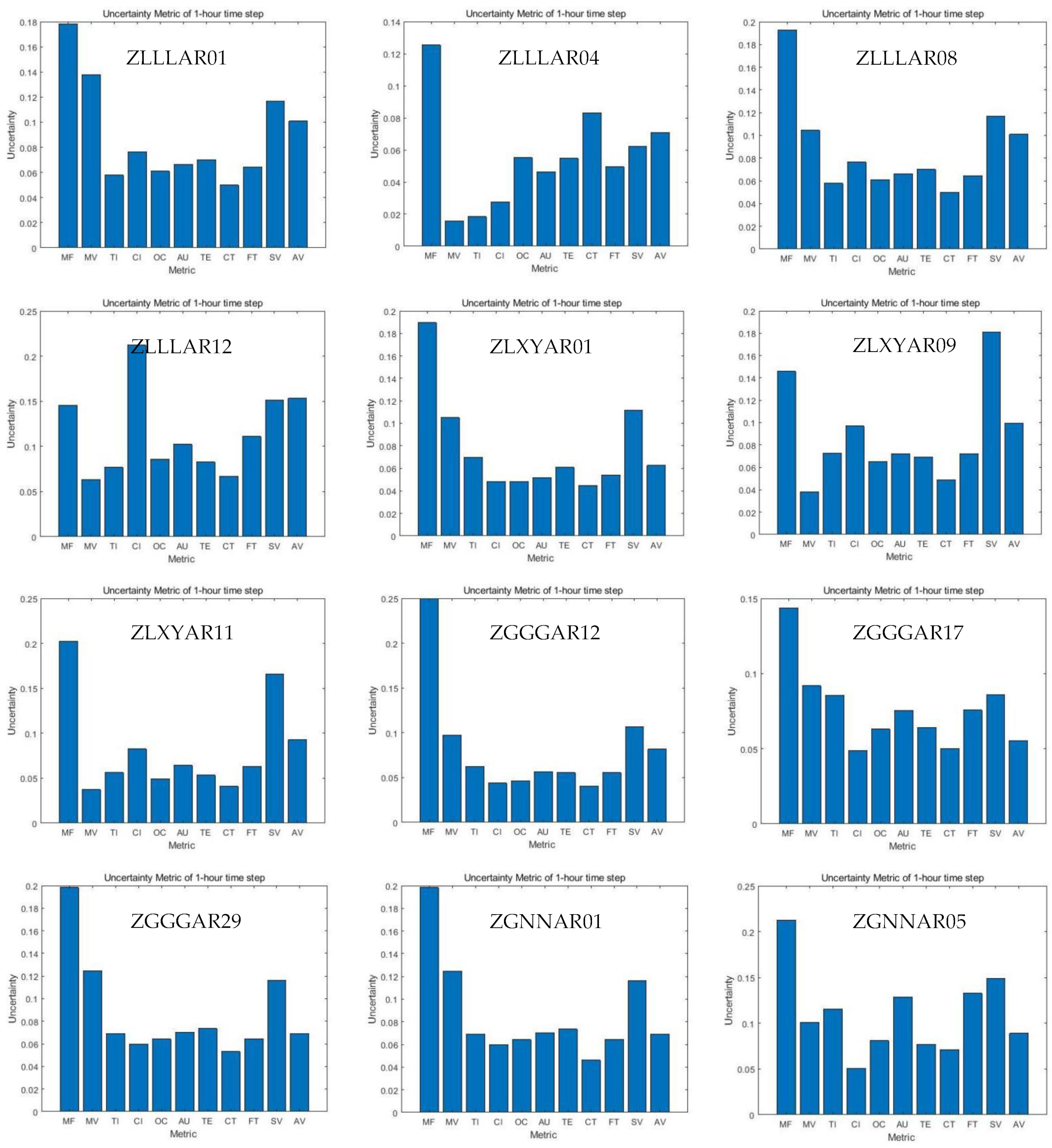
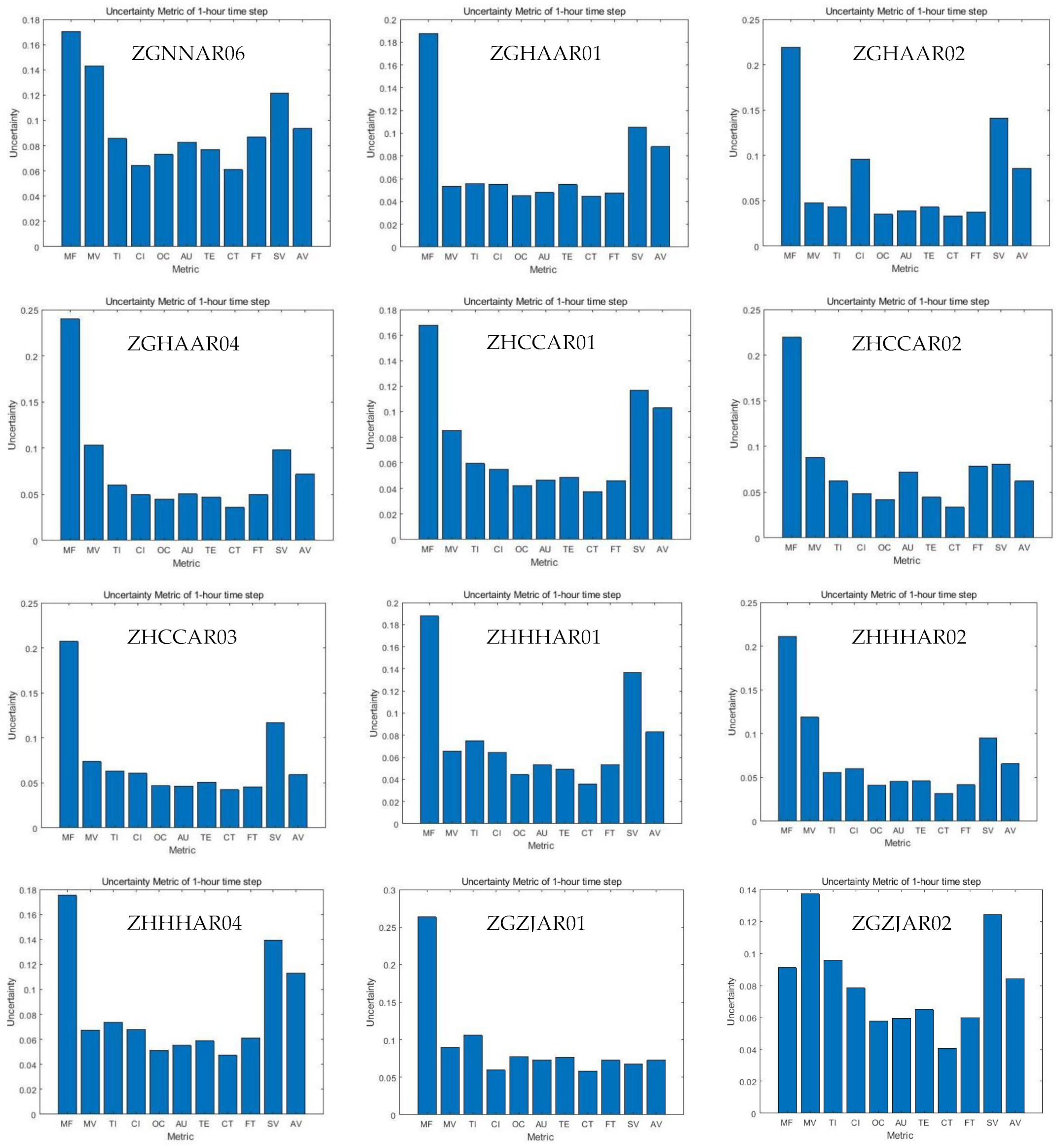
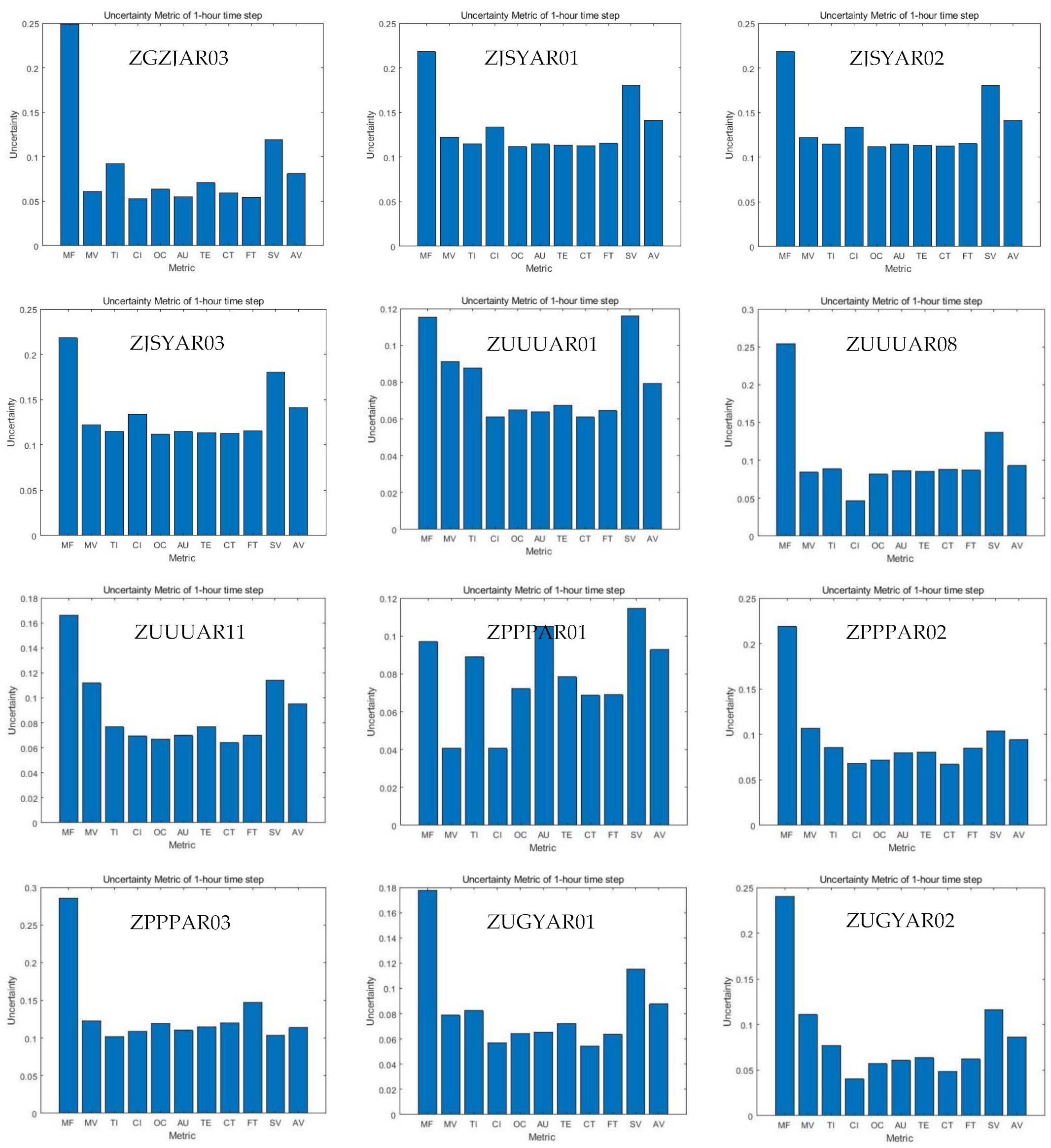
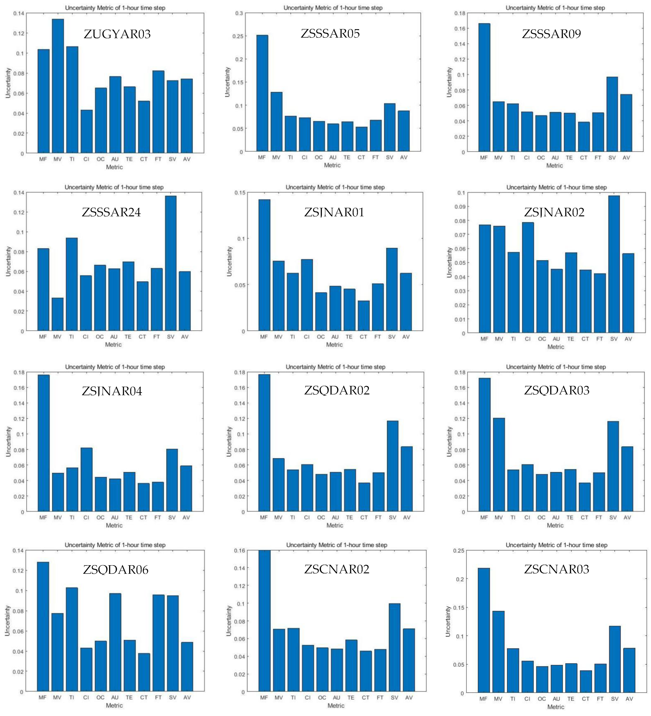
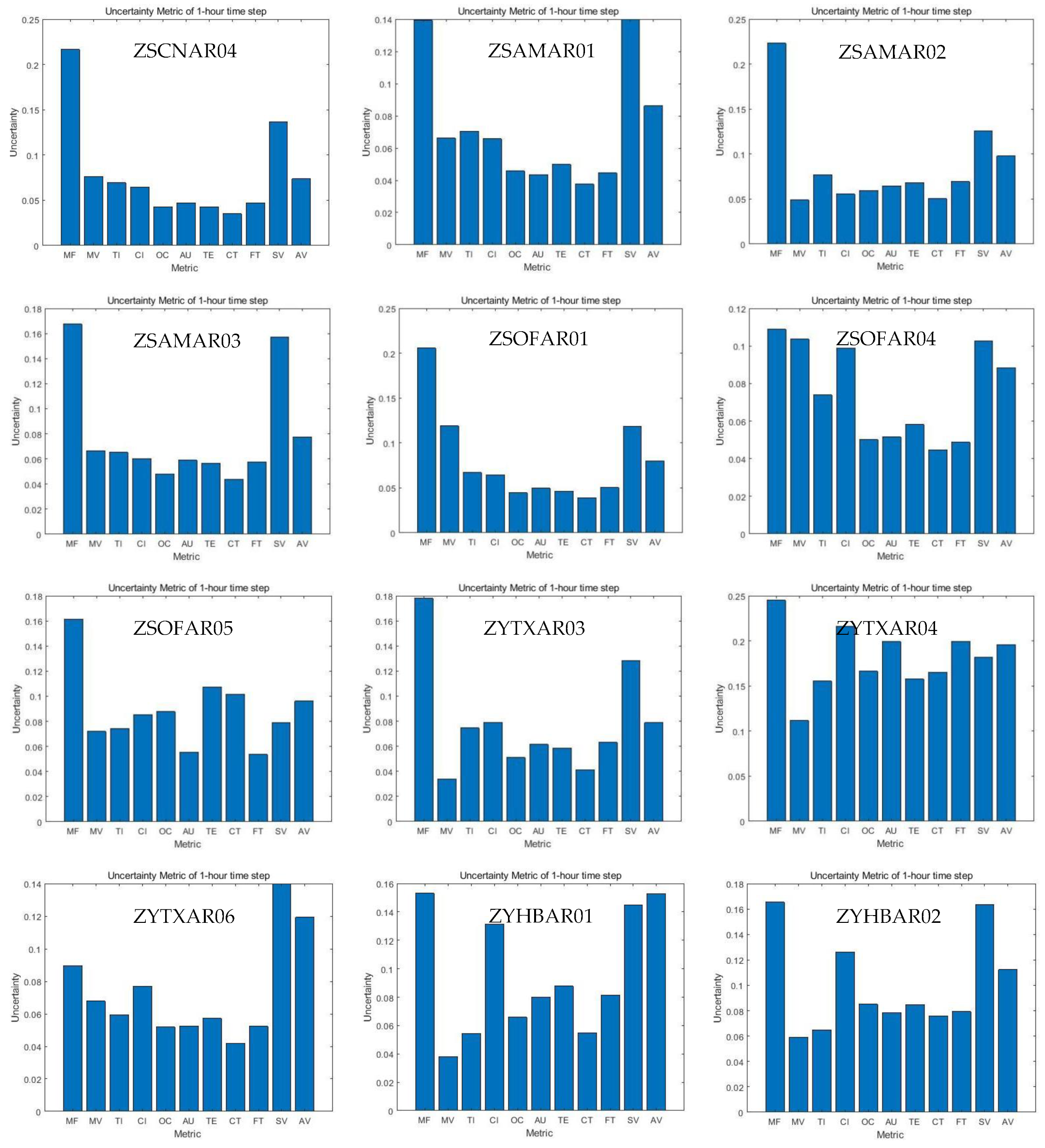
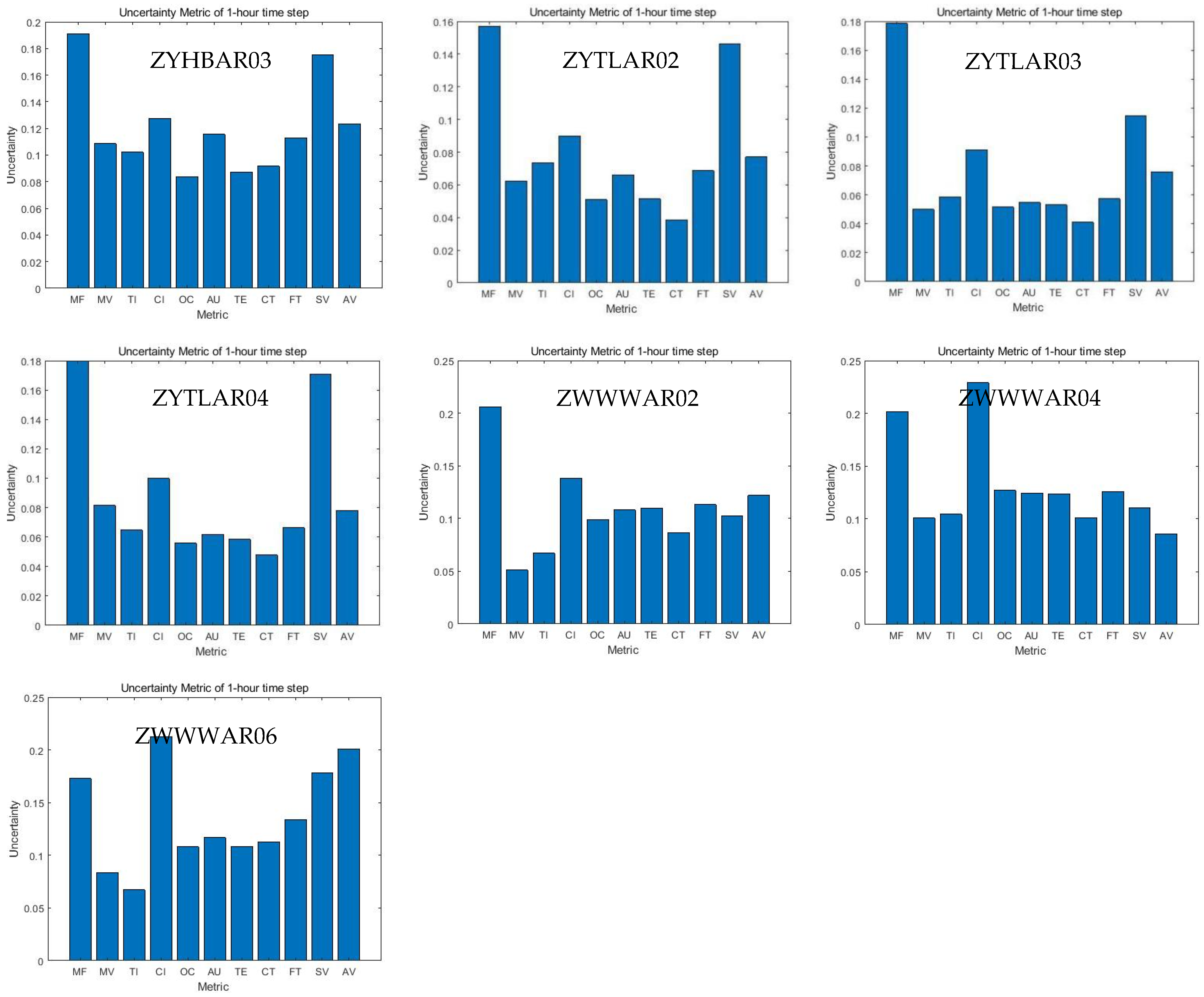
According to the statistical results of the airspace complexity indicators, the uncertainty of the corresponding complexity indicator is calculated. For the 25 Upper Control Areas of China, 3 typical sectors of each Upper Control Area are selected with high, medium, and low traffic volume respectively. Therefore, a total of 76 sectors are selected for the uncertainty analysis of airspace complexity indicators. Appendix A shows the uncertainties of the 76 sectors of complexity indicators.
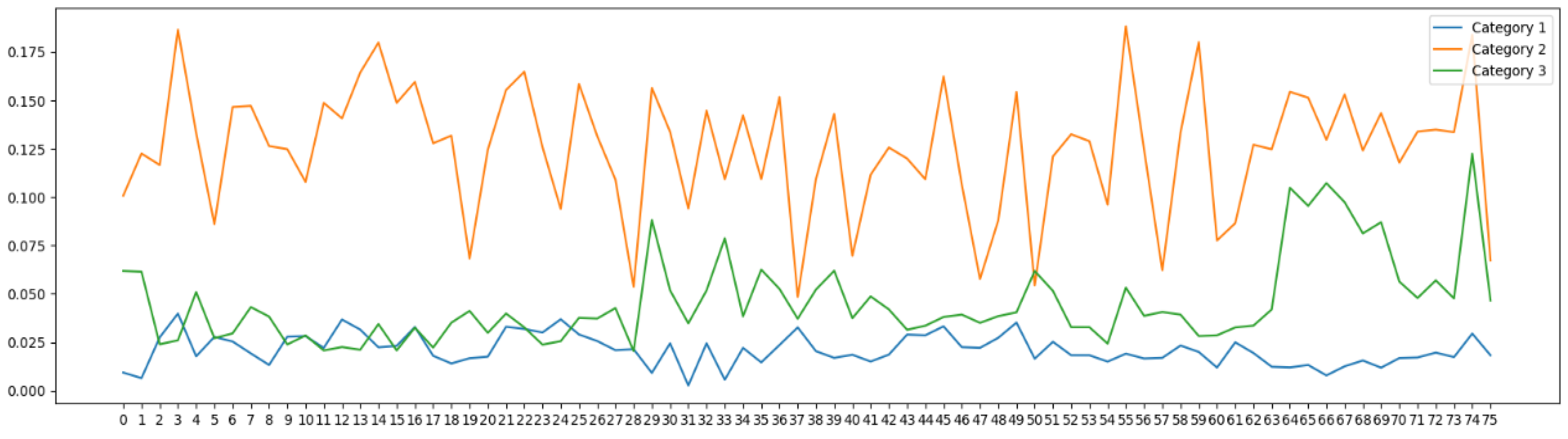
The K-Means clustering algorithm is used to cluster the complexity indicators above, where the feature of the clustering sample is the complexity indicator uncertainty of different sectors. In Appendix B, Table A1 shows the cluster labels for each complexity indicator, and Figure A2 shows the cluster centers.
Based on the K-Means clustering results and Table 3, the main traffic flow (MF) is classified as the high-level uncertainty indicator. Conflict Intensity (CI), Altitude Variation (AV), and Speed Variation (SV) can be classified as medium-level uncertainty indicators. Traffic Entry (TE), Occupancy (OC), Main Flow Variation (MV), Number of Trajectory Intersection (TI), The total flight time of the aircraft under ATCO responsibility in the given timeframe (FT), Airspace uses (AU), and Number of control transfers (CT) are classified as low-level uncertainty indicators. The uncertainty classification of the complexity indicators is shown in Table 3.
The simulation scenario is constructed using AirTOp and the control event parameters are corrected to generate a reliable workload training set. The calibrated event-based workload parameters are listed in Appendix C. The magnitude of the influence of complexity indicators on workload estimation is derived using the XGBoost algorithm, and the results are shown in Figure 8.
Based on the results of the complexity indicator uncertainty analysis and the results of the magnitude of influence on the ATC workload estimation, the final complexity indicator profile is shown in Table 4.
4.3. Validation of Workload Estimation
The indicators with lower uncertainty and higher impact were selected from Table 4 to build the ATC workload estimation model: CI, AV, TE, CT, TI, AU, OC, and FT.
The data set is divided, and 90% of it is selected as the training set and 10% as the test set. In order to quantitatively analyze and compare the estimation results of the models, the complex correlation coefficient , Root Mean Square Error (RMSE), and Mean Absolute Error (MAE) were used as indicators to evaluate the performance of the model. The calculation formula is as follows [59]:
In Equations (19)–(21), is the value of the variable (this study refers to ATC workload), is the actual value of controller workload; is the average value of ; is the predicted value of ; is the number of samples in the test set.
The evaluation results of estimation error are obtained, as shown in Table 5.
It can be seen from Table 5 that the of the model is higher, while the MAE and RMSE are smaller, so it has a better effect on the estimation of ATC workload.
The model accuracy of the estimation results and the actual ATC workload error in the range of ±2, ±4, ±6, ±8, and ±10 is shown in Table 6. It can be seen that within the error range of ±8, the estimation accuracy of the model can reach 94.956%.
4.4. Discussion of Results
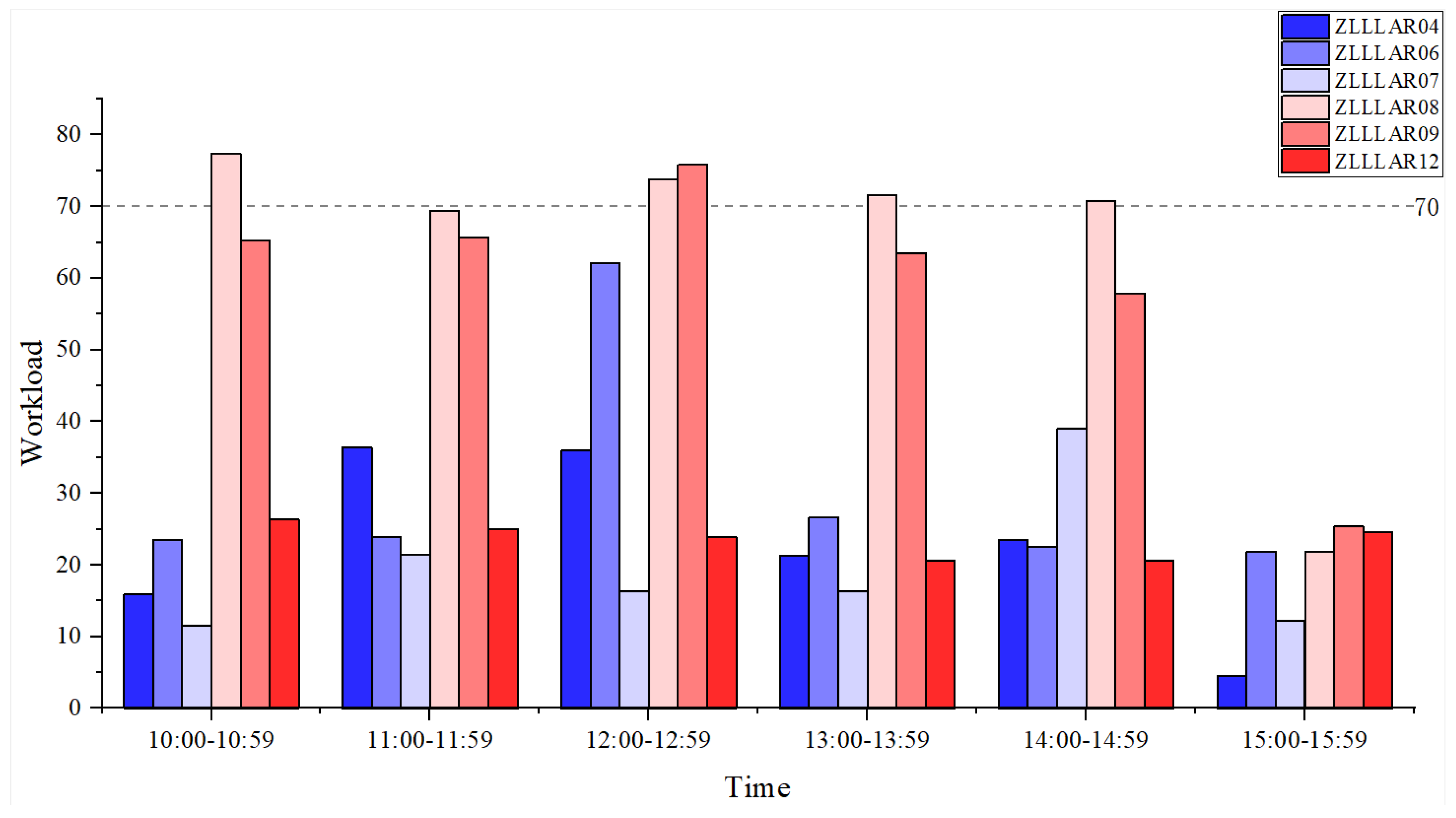
According to the ATC workload estimation model, Figure 9 shows the workload estimation results of each sector from 10:00 to 15:59 on 8 June 2019.
Three time periods, 10:00–11:59, 12:00–13:59, and 14:00–15:59, are selected for the sector partitioning experiment. Setting the sector workload threshold to 70, then in the period 10:00–11:59, ZLLLAR08 is overloaded; in the period 12:00–13:59, ZLLLAR08 and ZLLLAR09 are overloaded; in the period 14:00–15:59, ZLLLAR08 is overloaded. The overloaded sectors are combined with their adjacent sectors as the target airspace, and the BSP algorithm is used to partition them in the first stage.
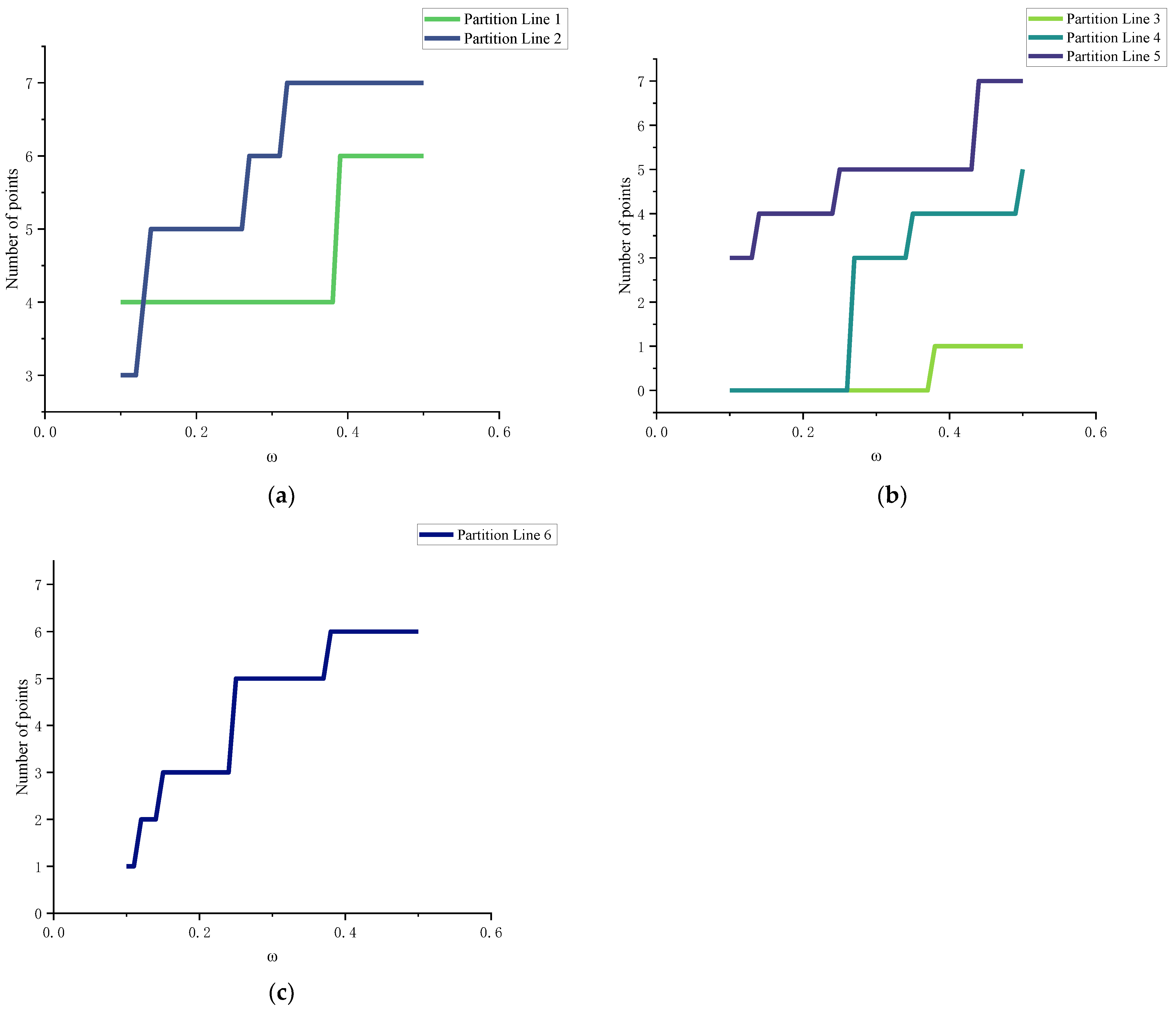
After obtaining the initial partition lines by the one-stage BSP algorithm, the sector boundaries can be further optimized by the A*-based heuristic algorithm. Figure 10 shows the relationship between the number of points connected to all sector partition lines and the weight values for all three time periods. As shown in Figure 10, with the increase of the weight , the more the number of points connected by the partition lines, the more the waypoints and known entry/exit points within the sector are used. In this way, it is more convenient for the ATC to control the aircraft operation and improve efficiency. The smaller the weight value , the smaller the number of points connected to the partition line, and the smoother the sector boundaries.
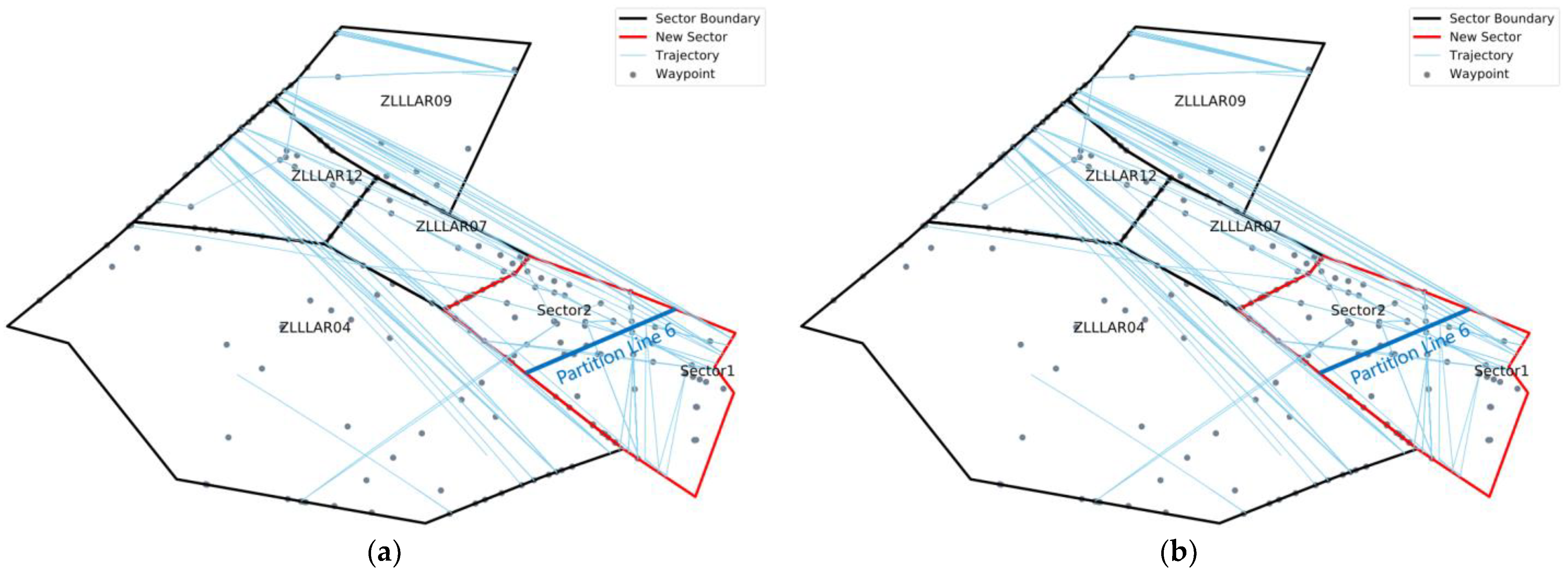
For the three time periods, we choose the weight value of 0.25 to optimize all the partition lines, taking into account the utilization rate of the points within the airspace as well as the smoothness of the sector boundaries. At the same time, it is still necessary to consider whether the optimized segmentation lines and new sectors satisfy the constraints of sector boundary optimization and the requirement that all workloads do not exceed the threshold. After experiments, at the weight value of 0.25, the sector workloads delineated by the optimized partition lines 2 and 6 exceed the threshold, so the one-stage division results are maintained; the rest of the lines meet all requirements.
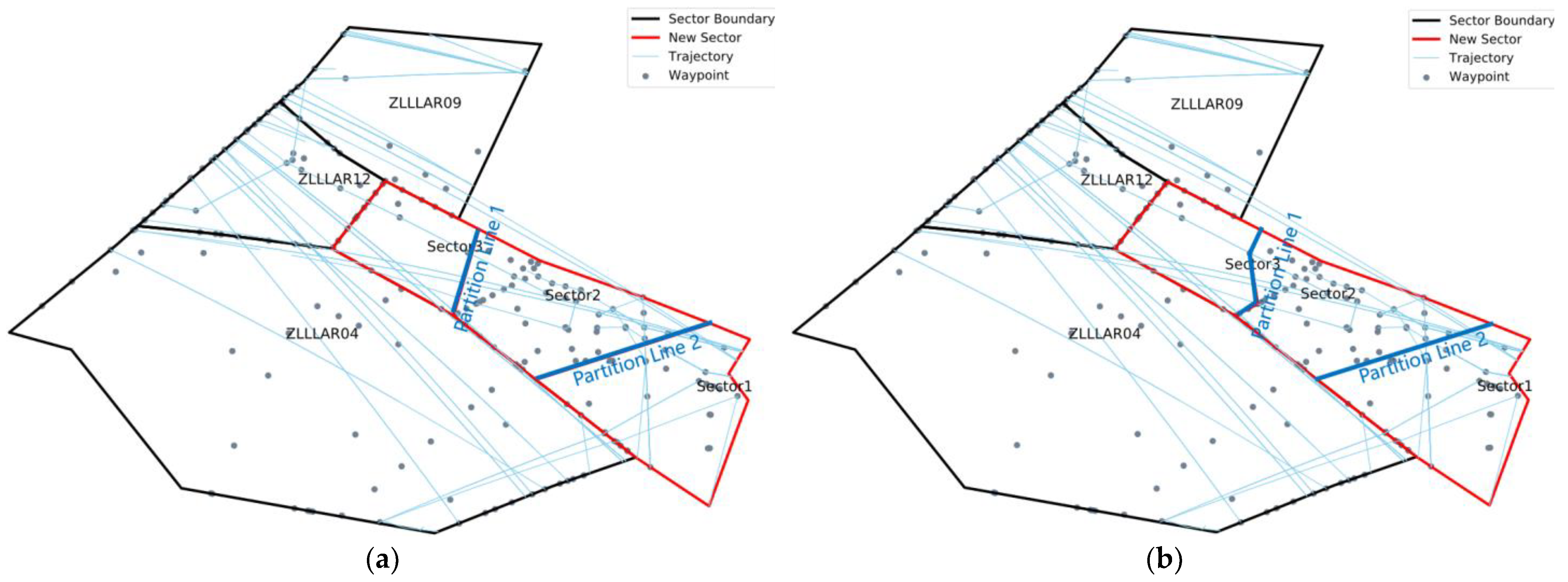
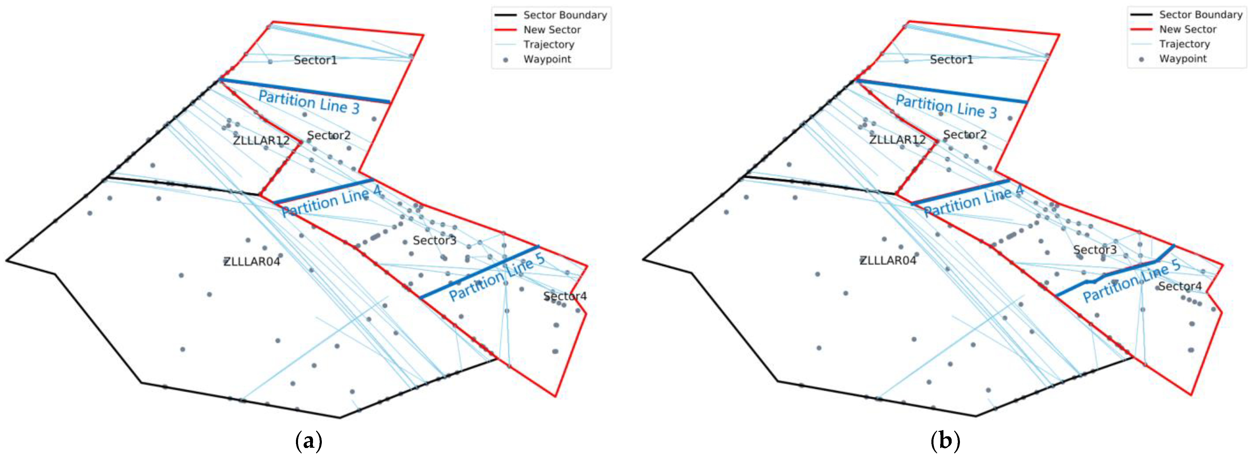
Figure 11a, Figure 12a and Figure 13a show the sector structure after the first stage of partition for the three time periods. Figure 11b, Figure 12b and Figure 13b show the sector boundary optimization results of the second stage. Table 7, Table 8 and Table 9 show the comparison of the workload of each sector before and after the division.
5. Conclusions
In this paper, we propose a DAC method applied to FRA to alleviate traffic capacity-demand imbalance and airspace congestion in pre-tactical phase. Firstly, the ATC workload of FRA sectors is estimated by constructing CIS considering uncertainty. Then a two-stage sector boundary optimization method is proposed. The target airspace is formed by combining the sectors that exceed the workload threshold with the adjacent sectors. The sector boundaries are automatically tuned using BSP and A*-based heuristic algorithms to conform to the FRA operational structure and the “direct to” feature. Finally, the effectiveness of the proposed method for balancing the ATC workload is verified by taking the Lanzhou regional control airspace in China as an example.
Nevertheless, one of the main drawbacks of the proposed methodology in this paper is that the quantified demand uncertainty level is only used to select complexity indicators, rather than providing probability distributions for probability workload estimation, which shall be included in further studies. In addition, the vertical boundaries of the sectors shall be also optimized using more advanced optimization algorithms [60,61].
For future practical implementation, it is essential to carefully validate the results by “Human-In-The Loop” simulation. Collecting real-time operation data including airspace usage, flight trajectory, air-ground communication, etc., is another way of monitoring, verifying, and improving the effectiveness of the overall methodology in a feedback loop. Moreover, a series of procedures and functions need to be upgraded to improve the safety and efficiency of dynamic sector management, e.g., the flexible use of airspace (FUA) procedures, air traffic flow probability prediction, ATC team resource management, airspace situation monitoring, etc.
Author Contributions
Conceptualization, L.Y., J.H., Q.G. and Y.Z.; methodology, L.Y., J.H., Q.G. and Y.Z.; validation, Q.G.; formal analysis, Y.Z. and J.H.; resources, M.H. and H.X.; data curation, H.X.; writing—original draft preparation, L.Y. and J.H.; writing—review and editing, L.Y., M.H. and H.X.; visualization, J.H. and Y.Z.; supervision, L.Y.; project administration, L.Y.; funding acquisition, L.Y. All authors have read and agreed to the published version of the manuscript.
Funding
This research was funded by the National Natural Science Foundation of China (Grant No.61903187, No.71731001), Natural Science Foundation of Jiangsu Province (Grant No. BK20190414).
Data Availability Statement
Not applicable.
Conflicts of Interest
The authors declare no conflict of interest.
Appendix A
Appendix A shows the uncertainty evaluation results of complexity indicators of 76 sectors in the China en-route airspace.
Figure A1.
The uncertainty evaluation results of complexity indicators of 76 sectors in the China en-route airspace.
Figure A1.
The uncertainty evaluation results of complexity indicators of 76 sectors in the China en-route airspace.


Appendix B
In Appendix B, Table A1 shows the cluster labels for each complexity indicator, and Figure A2 shows the cluster centers.

Table A1.
Cluster label of each complexity indicator.
| Cluster 1 | MF |
| Cluster 2 | CI |
| AV | |
| SV | |
| TE | |
| OC | |
| MV | |
| TI | |
| FT | |
| AU | |
| CT |
Figure A2.
Centers of the cluster.

Appendix C
In Appendix C, Table A2 shows the calibrated event-based workload parameters that were iteratively calibrated by three licensed air traffic controllers from Lanzhou ATC center. Through the iterated “parameter adjustment-simulation-comparison-parameter adjustment” process, the Pearson Correlation test indicates a high correlation of 0.957 between simulated and actual workload rated by controllers; the two-tailed probability passes the significance level test with a p-value of 0 < 0.01.
Table A2.
Main control events and their workload parameters set in AirTOp simulator.
| Event | Total Workload | Monitor | Air/Ground Communication | Height Statement | Conflict Detection | Conflict Resolution | Coordination |
|---|---|---|---|---|---|---|---|
| Sector Entry | 0:00:15 | 0:00:05 | 0:00:08 | 0:00:02 | |||
| Sector Exit | 0:00:10 | 0:00:08 | 0:00:02 | ||||
| Level Change | 0:00:08 | 0:00:08 | |||||
| Conflict Detection -crossing both cruising | 0:00:20 | 0:00:20 | |||||
| Conflict Detection—crossing both in vertical | 0:00:30 | 0:00:30 | |||||
| Conflict Detection—crossing one in vertical | 0:00:25 | 0:00:25 | |||||
| Conflict Detection—opposite both cruising | 0:00:20 | 0:00:20 | |||||
| Conflict Detection—opposite both in vertical | 0:00:30 | 0:00:30 | |||||
| Conflict Detection—opposite one in vertical | 0:00:25 | 0:00:25 | |||||
| Conflict Detection—same track both cruising | 0:00:10 | 0:00:10 | |||||
| Conflict Detection—same track both in vertical | 0:00:20 | 0:00:20 | |||||
| Conflict Detection—same track one in vertical | 0:00:15 | 0:00:15 | |||||
| Conflict Resolution—crossing both cruising | 0:00:40 | 0:00:40 | |||||
| Conflict Resolution—crossing both in vertical | 0:01:00 | 0:01:00 | |||||
| Conflict Resolution—crossing one in vertical | 0:00:45 | 0:00:45 | |||||
| Conflict Resolution—opposite both cruising | 0:01:10 | 0:01:10 | |||||
| Conflict Resolution—opposite both in vertical | 0:01:00 | 0:01:00 | |||||
| Conflict Resolution—opposite one in vertical | 0:00:50 | 0:00:50 | |||||
| Conflict Resolution—same track both cruising | 0:00:30 | 0:00:30 | |||||
| Conflict Resolution—same track both in vertical | 0:00:40 | 0:00:40 | |||||
| Conflict Resolution—same track one in vertical | 0:00:30 | 0:00:30 |
References
- Sergeeva, M. Automated Airspace Sectorization by Genetic Algorithm. Ph.D. Thesis, Université Paul Sabatier, Toulouse, France, 2017. [Google Scholar]
- Gaxiola, C.A.N.; Barrado, C.; Royo, P.; Pastor, E. Assessment of the North European free route airspace deployment. J. Air Transp. Manag. 2018, 73, 113–119. [Google Scholar] [CrossRef]
- Eurocontrol. Network Performance Plan 2020–2024; Eurocontrol: Brussels, Belgium, 2022. [Google Scholar]
- Kopardekar, P.; Bilimoria, K.; Sridhar, B. Initial concepts for dynamic airspace configuration. In Proceedings of the 7th AIAA ATIO Conference, 2nd CEIAT International Conference on Innovation and Integrity in Aero Sciences, 17th LTA Systems Tech Conference; Followed by 2nd TEOS Forum, Belfast, Ireland, 18–20 September 2017; AIAA: Belfast, Ireland, 2007; p. 7763. [Google Scholar]
- Hind, H.; El Omri, A.; Abghour, N.; Moussaid, K.; Rida, M. Dynamic airspace configuration: Review and open research issues. In Proceedings of the 2018 4th International Conference on Logistics Operations Management (GOL), Le Havre, France, 10–12 April 2018; pp. 1–7. [Google Scholar]
- Rahman, S.M.A.; Borst, C.; Mulder, M.; van Paassen, R. Sector complexity measures: A comparison. J. Teknol. 2015, 76, 131–139. [Google Scholar]
- Xie, H.; Zhang, M.; Ge, J.; Dong, X.; Chen, H. Learning air traffic as images: A deep convolutional neural network for airspace operation complexity evaluation. Complexity 2021, 2021, 6457246. [Google Scholar] [CrossRef]
- Kudumija, D.; Antulov-Fantulin, B.; Andraši, P.; Rogošić, T. The effect of the Croatian Free Route Airspace implementation on the Air Traffic Complexity. Transp. Res. Procedia 2022, 64, 356–363. [Google Scholar] [CrossRef]
- Cao, X.; Zhu, X.; Tian, Z.; Chen, J.; Wu, D.; Du, W. A knowledge-transfer-based learning framework for airspace operation complexity evaluation. Transp. Res. Part C Emerg. Technol. 2018, 95, 61–81. [Google Scholar] [CrossRef]
- García, A.; Delahaye, D.; Soler, M. Air traffic complexity map based on linear dynamical systems. Aerospace 2022, 9, 230. [Google Scholar]
- Isufaj, R.; Omeri, M.; Piera, M.A.; Saez Valls, J.; Verdonk Gallego, C. From Single Aircraft to Communities: A Neutral Interpretation of Air Traffic Complexity Dynamics. Aerospace 2022, 9, 613. [Google Scholar] [CrossRef]
- Manning, C.A.; Pfleiderer, E.M. Relationship of Sector Activity and Sector Complexity to Air Traffic Controller Taskload; Department of Transportation; Federal Aviation Administration: Washington, DC, USA, 2006. [Google Scholar]
- Gianazza, D.; Guittet, K. Selection and evaluation of air traffic complexity metrics. In Proceedings of the 2006 IEEE/AIAA 25TH Digital Avionics Systems Conference, Portland, OR, USA, 15–18 October 2006; pp. 1–12. [Google Scholar]
- Gianazza, D. Forecasting workload and airspace configuration with neural networks and tree search methods. Artif. Intell. 2010, 174, 530–549. [Google Scholar] [CrossRef] [Green Version]
- Loft, S.; Sanderson, P.; Neal, A.; Mooij, M. Modeling and predicting mental workload in en route air traffic control: Critical review and broader implications. Hum. Factors 2007, 49, 376–399. [Google Scholar] [CrossRef] [Green Version]
- Marr, B.; Lindsay, K. Controller workload-based calculation of monitor alert parameters for en route sectors. In Proceedings of the 15th AIAA Aviation Technology, Integration, and Operations Conference, Dallas, TX, USA, 22–26 June 2015; p. 3178. [Google Scholar]
- Yousefi, A.; Donohue, G. Temporal and spatial distribution of airspace complexity for air traffic controller workload-based sectorization. In Proceedings of the AIAA 4th Aviation Technology, Integration and Operations (ATIO) Forum, Los Angeles, CA, USA, 20 September 2004; p. 6455. [Google Scholar]
- Kulkarni, S.; Ganesan, R.; Sherry, L. Static sectorization approach to dynamic airspace configuration using approximate dynamic programming. In Proceedings of the 2011 Integrated Communications, Navigation, and Surveillance Conference Proceedings, Herndon, VA, USA, 10–12 May 2011; pp. J2-1–J2-9. [Google Scholar]
- Faulkner, L.; McFadyen, A. Air Traffic Configuration Modelling and Dynamic Airspace Allocation using Discrete-Time Markov Chains. In Proceedings of the 2019 IEEE Intelligent Transportation Systems Conference (ITSC), Auckland, New Zealand, 27–30 October 2019; pp. 4483–4488. [Google Scholar]
- Temizkan, S.; SİPahİOĞLu, A. A mathematical model suggestion for airspace sector design. J. Fac. Eng. Archit. Gazi Univ. 2016, 31, 4. [Google Scholar]
- Mohammed, G.; El Bekkaye, M. Fuzzy Dynamic Airspace Sectorization Problem. In Machine Intelligence and Data Analytics for Sustainable Future Smart Cities; Springer: Berlin/Heidelberg, Germany, 2021; pp. 229–250. [Google Scholar]
- Wei, J.; Hwang, I.; Hall, W. Mathematical programming based algorithm for dynamic terminal airspace configuration. In Proceedings of the 12th AIAA Aviation Technology, Integration, and Operations (ATIO) Conference and 14th AIAA/ISSMO Multidisciplinary Analysis and Optimization Conference, Indianapolis, IN, USA, 17–19 September 2012. [Google Scholar]
- Wei, J.; Sciandra, V.J.; Hwang, I.; Hall, W.D. An integer programming based sector design algorithm for terminal dynamic airspace configuration. In Proceedings of the 2013 Aviation Technology, Integration, and Operations Conference, Los Angeles, CA, USA, 12–14 August 2013; p. 4260. [Google Scholar]
- Wei, J.; Sciandra, V.; Hwang, I.; Hall, W.D. Design and evaluation of a dynamic sectorization algorithm for terminal airspace. J. Guid. Control Dyn. 2014, 37, 1539–1555. [Google Scholar] [CrossRef]
- Klein, A.; Rodgers, M.D.; Kaing, H. Dynamic FPAs: A new method for dynamic airspace configuration. In Proceedings of the 2008 Integrated Communications, Navigation and Surveillance Conference, Bethesda, MD, USA, 5–7 May 2008; pp. 1–11. [Google Scholar]
- Xue, M. Airspace sector redesign based on Voronoi diagrams. J. Aerosp. Comput. Inf. Commun. 2009, 6, 624–634. [Google Scholar] [CrossRef]
- Yousefi, A.; Khorrami, B.; Hoffman, R.; Hackney, B. Enhanced Dynamic Airspace Configuration Algorithms and Concepts; Technical Report No. 34N1207-001-R0; Metron Aviation Inc.: Herndon, VA, USA, 2007. [Google Scholar]
- Basu, A.; Mitchell, J.S.; Sabhnani, G.K. Geometric algorithms for optimal airspace design and air traffic controller workload balancing. J. Exp. Algorithm. 2010, 14, 2.3–2.28. [Google Scholar]
- Tang, J.; Alam, S.; Lokan, C.; Abbass, H.A. A multi-objective approach for dynamic airspace sectorization using agent based and geometric models. Transp. Res. Part C Emerg. Technol. 2012, 21, 89–121. [Google Scholar] [CrossRef]
- Li, J.; Wang, T.; Savai, M.; Hwang, I. Graph-based algorithm for dynamic airspace configuration. J. Guid. Control Dyn. 2010, 33, 1082–1094. [Google Scholar] [CrossRef]
- Cao, H.; Wu, X.; Zhou, F.; Wang, T. Dynamic airspace sector configuration based on bi-partitioned method. In Proceedings of the 2015 7th International Conference on Modelling, Identification and Control (ICMIC), Sousse, Tunisia, 18–20 December 2015; pp. 1–4. [Google Scholar]
- Ghorpade, S. Airspace configuration model using swarm intelligence based graph partitioning. In Proceedings of the 2016 IEEE Canadian Conference on Electrical and Computer Engineering (CCECE), Vancouver, BC, Canada, 15–18 May 2016; pp. 1–5. [Google Scholar]
- Zou, X.; Cheng, P.; An, B.; Song, J. Sectorization and configuration transition in airspace design. Math. Probl. Eng. 2016, 2016, 6048326. [Google Scholar] [CrossRef] [Green Version]
- Yao, D.; Wang, Y. Two-Stage Model and Algorithm for Airspace and Traffic Flow Collaborative Programming Based on Dynamic Sectorization. J. Northwest. Polytech. Univ. 2016, 34, 549–557. [Google Scholar]
- Brinton, C.R.; Pledgie, S. Airspace partitioning using flight clustering and computational geometry. In Proceedings of the 2008 IEEE/AIAA 27th Digital Avionics Systems Conference, Salt Lake City, UT, USA, 26–30 October 2008; pp. 3. B. 3-1–3. B. 3-10. [Google Scholar]
- Kopardekar, P.; Magyarits, S. Measurement and prediction of dynamic density. In Proceedings of the 5th USA/Europe Air Traffic Management R&D Seminar, Budapest, Hungary, 23–27 June 2003. [Google Scholar]
- Lucic, P.; Klein, A.; Leiden, K.; Brinton, C. A template-based approach to Dynamic Airspace Configuration in presence of weather. In Proceedings of the 2013 IEEE/AIAA 32nd Digital Avionics Systems Conference (DASC), East Syracuse, NY, USA, 5–10 October 2013; pp. 1D5-1–1D5-14. [Google Scholar]
- Martinez, S.; Chatterji, G.; Sun, D.; Bayen, A. A weighted-graph approach for dynamic airspace configuration. In Proceedings of the Aiaa Guidance, Navigation and Control Conference and Exhibit, Hilton Head, SC, USA, 20–23 August 2007; p. 6448. [Google Scholar]
- Gerdes, I.; Temme, A.; Schultz, M. Dynamic airspace sectorization using controller task load. In Proceedings of the 6th SESAR Innovation Days, Delft, The Netherlands, 8–10 November 2016. [Google Scholar]
- Gerdes, I.; Temme, A.; Schultz, M. Dynamic airspace sectorisation for flight-centric operations. Transp. Res. Part C Emerg. Technol. 2018, 95, 460–480. [Google Scholar] [CrossRef]
- Standfuß, T.; Gerdes, I.; Temme, A.; Schultz, M. Dynamic airspace optimisation. CEAS Aeronaut. J. 2018, 9, 517–531. [Google Scholar] [CrossRef]
- Chen, Y.; Zhang, D. Dynamic airspace configuration method based on a weighted graph model. Chin. J. Aeronaut. 2014, 27, 903–912. [Google Scholar] [CrossRef] [Green Version]
- Lema-Esposto, M.F.; Amaro-Carmona, M.Á.; Valle-Fernández, N.; Iglesias-Martínez, E.; Fabio-Bracero, A. Optimal Dynamic Airspace Configuration (DAC) based on State-Task Networks (STN). In Proceedings of the 11th SESAR Innovation Days, Online, 7–9 December 2021. [Google Scholar]
- Sergeeva, M.; Delahaye, D.; Zerrouki, L.; Schede, N. Dynamic airspace configurations generated by evolutionary algorithms. In Proceedings of the 2015 IEEE/AIAA 34th Digital Avionics Systems Conference (DASC), Prague, Czech Republic, 13–17 September 2015; pp. 1F2-1–1F2-15. [Google Scholar]
- Sergeeva, M.; Delahaye, D.; Mancel, C.; Vidosavljevic, A. Dynamic airspace configuration by genetic algorithm. J. Traffic Transp. Eng. 2017, 4, 300–314. [Google Scholar] [CrossRef]
- Liu, J.; Lan, S.; Jiang, H.; Xu, C. Research on Situational Awareness of Controllers based on Human Factors. Chin. J. Ergon. 2021, 27, 51–56. [Google Scholar]
- Li, H.; Wang, Y.-P. Research on Sector Dynamic Traffic Capacity Based on Airspace Complexity. Aeronaut. Comput. Tech. 2019, 49, 79–83. [Google Scholar]
- Gomez Comendador, V.F.; Arnaldo Valdés, R.M.; Vidosavljevic, A.; Sanchez Cidoncha, M.; Zheng, S. Impact of trajectories’ uncertainty in existing ATC complexity methodologies and metrics for DAC and FCA SESAR concepts. Energies 2019, 12, 1559. [Google Scholar] [CrossRef] [Green Version]
- Gomez Comendador, V.F.; Arnaldo Valdés, R.M.; Villegas Diaz, M.; Puntero Parla, E.; Zheng, D. Bayesian network modelling of ATC complexity metrics for future SESAR demand and capacity balance solutions. Entropy 2019, 21, 379. [Google Scholar] [CrossRef] [Green Version]
- Cong, W.; Hu, M.H.; Xie, H.; Zhang, C. An Evaluation Method of Sector Complexity Based on Metrics System. J. Transp. Syst. Eng. Inf. Technol. 2015, 15, 136. [Google Scholar]
- Djokic, J.; Lorenz, B.; Fricke, H. Air traffic control complexity as workload driver. Transp. Res. Part C Emerg. Technol. 2010, 18, 930–936. [Google Scholar] [CrossRef]
- Li, S.; Qin, J.; He, M.; Paoli, R. Fast Evaluation of Aircraft Icing Severity Using Machine Learning Based on XGBoost. Aerospace 2020, 7, 36. [Google Scholar] [CrossRef]
- Wang, Y. Research on Airspace Sector Dynamic Planning and Optimization. Master’s Thesis, Civil Aviation University of China, Tianjin, China, 2020. [Google Scholar]
- Sherali, H.D.; Hill, J.M. Configuration of airspace sectors for balancing air traffic controller workload. Ann. Oper. Res. 2013, 203, 3–31. [Google Scholar] [CrossRef]
- Zhang, M. Research on Key Problems of Terminal Airspace’s Sector Planning and Operation Management; Nanjing University of Aeronautics and Astronautics: Nanjing, China, 2010. [Google Scholar]
- Wang, C.; Chen, Y. Large-scale airspace sector partitioning based on binary space partitions and dynamic programming. Appl. Res. Comput. 2015, 32, 3259–3263. [Google Scholar]
- Mitchell, J.; Sabhnani, G.; Hoffman, R.; Krozel, J.; Yousefi, A. Dynamic airspace configuration management based on computational geometry techniques. In Proceedings of the AIAA Guidance, Navigation and Control Conference and Exhibit, Monterey, CA, USA, 5–8 August 2008; p. 7225. [Google Scholar]
- Chen, J.; Leung, M.K.; Gao, Y. Noisy logo recognition using line segment Hausdorff distance. Pattern Recognit. 2003, 36, 943–955. [Google Scholar] [CrossRef] [Green Version]
- Zhao, Z.; Feng, S.; Song, M.; Hu, L.; Lu, S. Prediction method of aircraft dynamic taxi time based on XGBoost. Adv. Aeronaut. Sci. Eng. 2022, 13, 76–85. [Google Scholar]
- Nguyen, T.V.; Huynh, N.-T.; Vu, N.-C.; Kieu, V.N.; Huang, S.-C. Optimizing compliant gripper mechanism design by employing an effective bi-algorithm: Fuzzy logic and ANFIS. Microsyst. Technol. 2021, 27, 3389–3412. [Google Scholar] [CrossRef]
- Wang, C.-N.; Yang, F.-C.; Nguyen, V.T.T.; Vo, N.T.M. CFD analysis and optimum design for a centrifugal pump using an effectively artificial intelligent algorithm. Aerospace 2022, 13, 1208. [Google Scholar] [CrossRef]
Figure 1.
Flowchart of sector workload estimation based on XGBoost.

Figure 2.
Flowchart of two-stage boundary generation and tuning in FRA.

Figure 3.
BSP algorithm flow chart.

Figure 4.
Angle distance illustration.

Figure 5.
Vertical distance, parallel distance illustration.

Figure 6.
A*-based heuristic algorithm process.

Figure 7.
Lanzhou regional control airspace scenarios.

Figure 8.
The magnitude of influence of complexity indicators on workload estimation.

Figure 9.
Lanzhou regional control airspace 8 June 2019 10:00–15:59 hourly workload forecast results for each sector.
Figure 9.
Lanzhou regional control airspace 8 June 2019 10:00–15:59 hourly workload forecast results for each sector.

Figure 10.
(a) The relationship between the number of points connected by partition line 1–2 and ; (b) The relationship between the number of points connected by partition line 3–5 and ; (c) The relationship between the number of points connected by partition line 6 and .
Figure 10.
(a) The relationship between the number of points connected by partition line 1–2 and ; (b) The relationship between the number of points connected by partition line 3–5 and ; (c) The relationship between the number of points connected by partition line 6 and .

Figure 11.
(a) 10:00–11:59 After one-stage; (b) 10:00–11:59 After two-stage.

Figure 12.
(a) 12:00–13:59 After one-stage; (b) 12:00–13:59 After two-stage.

Figure 13.
(a) 14:00–15:59 After one-stage; (b) 14:00–15:59 After two-stage.

Table 1.
CIS.
| Complexity Indicator | Abbreviation | Note |
|---|---|---|
| Number of Main Flows [47] | MF | |
| Main Flow Variation | MV | the standard deviation of the distribution of flight volume over the main traffic flows |
| Number of Trajectory Intersection | TI | the number of track intersections formed by the intersection of aircraft trajectories |
| Conflict Intensity | CI | the value of conflict intensity between aircraft pairs increases as the spatial distance between aircraft pairs decreases |
| Airspace uses [49] | AU | |
| Altitude Variation | AV | the standard deviation of the flight altitude for all aircraft |
| Speed Variation | SV | the standard deviation of flight speed for all aircraft |
| Occupancy (per ATCO position) | OC | the number of aircrafts at a given time instant |
| Traffic Entry (per ATCO position) [50] | TE | |
| The total flight time of the aircraft under ATCO responsibility in the given timeframe | FT | the controlled flight time for all aircraft |
| Number of control transfers [51] | CT |
Table 2.
Experimental parameters setting.
| Experimental Parameter Name | Value |
|---|---|
| Maximum number of intersections between the route and the sector boundaries | 2 pcs |
| Time required for the execution of a single control transfer | 5 min |
| The shortest distance between the route intersection and the sector boundary | 10,000 m |
| Minimum intersection angle between route and sector boundary | |
| Minimum Sector Horizontal-to-vertical Ratio | 0.3 |
Table 3.
Uncertainty classification of the complexity indicators.
| High-Level Indicator | MF |
|---|---|
| Medium-level Indicator | CI AV SV |
| Low-level Indicator | TE |
| OC MV TI FT AU CT |
Table 4.
Overall picture of complexity indicators.
| Low Impact | Medium Impact | High Impact | |
|---|---|---|---|
| High uncertainty | MF | ||
| Medium uncertainty | SV | CI | |
| AV | |||
| Low uncertainty | MV | TE | TI AU |
| CT | OC | ||
| FT |
Table 5.
Evaluation results of ATC workload estimation model based on XGBoost.
| Evaluation Parameters | Evaluation Result |
|---|---|
| RMSE | 11.16817 |
| MAE | 6.80012 |
| 0.89597 |
Table 6.
Estimation accuracy of ATC workload.
| Error | ±2 | ±4 | ±6 | ±8 | ±10 |
| Accuracy | 43.635% | 60.447 | 81.692% | 94.956% | 96.884% |
Table 7.
10:00–11:59 Workload values for each sector before and after optimization.
| Before | After One-Stage | After Two-Stage | |||||
|---|---|---|---|---|---|---|---|
| 10:00–10:59 | 11:00–11:59 | 10:00–10:59 | 11:00–11:59 | 10:00–10:59 | 11:00–11:59 | ||
| ZLLLAR06 | 23.5529 | 23.8674 | Sector 1 | 68.8843 | 60.4926 | 68.8843 | 60.4926 |
| ZLLLAR07 | 11.5431 | 21.3622 | Sector 2 | 65.5155 | 58.6889 | 65.5155 | 58.6889 |
| ZLLLAR08 | 77.3584 | 69.3848 | Sector 3 | 14.9662 | 12.2904 | 14.9662 | 12.2904 |
Table 8.
12:00–13:59 Workload values for each sector before and after optimization.
| Before | After One-Stage | After Two-Stage | |||||
|---|---|---|---|---|---|---|---|
| 12:00–12:59 | 13:00–13:59 | 12:00–12:59 | 13:00–13:59 | 12:00–12:59 | 13:00–13:59 | ||
| ZLLLAR06 | 62.0566 | 26.6573 | Sector 1 | 23.8674 | 65.2802 | 23.8674 | 65.2802 |
| ZLLLAR07 | 16.336 | 16.336 | Sector 2 | 63.8403 | 57.8604 | 63.8403 | 57.8604 |
| ZLLLAR08 | 73.7572 | 71.565 | Sector 3 | 69.565 | 51.9123 | 68.7609 | 51.9123 |
| ZLLLAR09 | 75.7915 | 63.5467 | Sector 4 | 68.5118 | 59.1439 | 68.5118 | 59.9098 |
Table 9.
14:00–15:59 Workload values for each sector before and after optimization.
| Before | After One-Stage | After Two-Stage | |||||
|---|---|---|---|---|---|---|---|
| 14: 00–14:59 | 15:00–15:59 | 14: 00–14:59 | 15:00–15:59 | 14: 00–14:59 | 15:00–15:59 | ||
| ZLLLAR06 | 22.5844 | 21.813 | Sector 1 | 69.142 | 37.879 | 69.142 | 37.879 |
| ZLLLAR08 | 70.7609 | 21.813 | Sector 2 | 23.8674 | 21.813 | 23.8674 | 21.813 |
Publisher’s Note: MDPI stays neutral with regard to jurisdictional claims in published maps and institutional affiliations. |
© 2022 by the authors. Licensee MDPI, Basel, Switzerland. This article is an open access article distributed under the terms and conditions of the Creative Commons Attribution (CC BY) license (https://creativecommons.org/licenses/by/4.0/).
Share and Cite
MDPI and ACS Style
Yang, L.; Huang, J.; Gao, Q.; Zhou, Y.; Hu, M.; Xie, H. Dynamic Boundary Optimization of Free Route Airspace Sectors. Aerospace 2022, 9, 832. https://doi.org/10.3390/aerospace9120832
AMA Style
Yang L, Huang J, Gao Q, Zhou Y, Hu M, Xie H. Dynamic Boundary Optimization of Free Route Airspace Sectors. Aerospace. 2022; 9(12):832. https://doi.org/10.3390/aerospace9120832
Chicago/Turabian StyleYang, Lei, Jue Huang, Qi Gao, Yi Zhou, Minghua Hu, and Hua Xie. 2022. "Dynamic Boundary Optimization of Free Route Airspace Sectors" Aerospace 9, no. 12: 832. https://doi.org/10.3390/aerospace9120832
Note that from the first issue of 2016, this journal uses article numbers instead of page numbers. See further details here.