An M^[X]/G(a,b)/1 Queueing System with Breakdown and Repair, Stand-By Server, Multiple Vacation and Control Policy on Request for Re-Service

Abstract

In this paper, we discuss a non-Markovian batch arrival general bulk service single-server queueing system with server breakdown and repair, a stand-by server, multiple vacation and re-service. The main server’s regular service time, re-service time, vacation time and stand-by server’s service time are followed by general distributions and breakdown and repair times of the main server with exponential distributions. There is a stand-by server which is employed during the period in which the regular server remains under repair. The probability generating function of the queue size at an arbitrary time and some performance measures of the system are derived. Extensive numerical results are also illustrated.

1. Introduction

Queueing systems with general bulk service and vacations have been studied by many researchers because they deal with effective utilization of the server’s idle time for secondary jobs. Such queueing systems have a wide range of application in many real-life situations such as production line systems, inventory systems, digital communications and computer networks. Doshi [1] and Takagi [2] have made a comprehensive survey of queueing systems with vacations. A batch arrival $M^{\left[X\right]}/G/1$ queueing system with multiple vacations was first studied by Baba [3]. Krishna Reddy et al. [4] have discussed an $M^{\left[X\right]}/G(a,b)/1$ model with an N-policy, multiple vacations and setup times. Jeyakumar and Senthilnathan [5] analyzed the bulk service queueing system with multiple working vacations and server breakdown.

The first work on re-service was done by Madan [6]. He consider an M/G /1 queueing model, in which the server performs the first essential service for all arriving customers. As soon as the first service is executed, they may leave the system with probability $(1-\theta )$, and the second optional service is provided with $\theta$. Madan et al. [7] considered a bulk arrival queue with optional re-service. Jeyakumar and Arumuganathan [8] discussed a bulk queue with multiple vacation and a control policy on request for re-service. Recently, Haridass and Arumuganathan [9] analyzed a batch service queueing system with multiple vacations, setup times and server choice of admitting re-service.

No system is found to be perfect in the real world, since all the devices fail more or less frequently. Thus, the random failures and systematic repair of components of a machining system have a significant impact on the output and the productivity of the machining system. A detailed survey on queues with interruptions was undertaken by Krishnamoorthy et al. [10]. Ayyappan and Shyamala [11] derived the transient solution to an $M^{\left[X\right]}/G/1$ queueing system with feedback, random breakdowns, Bernoulli schedule server vacation and random setup time. An M/G/1 queue with two phases of service subject to random breakdown and delayed repair was examined by Choudhury and Tadj [12]. Senthilnathan and Jeyakumar [13] studied the behavior of the server breakdown without interruption in an $M^{\left[X\right]}/G(a,b)/1$ queueing system with multiple vacations and closedown time. An M/G/1 two-phase multi-optional retrial queue with Bernoulli feedback, non-persistent customers and breakdown and repair was analyzed by Lakshmi and Ramanath [14]. Recently, a discrete time queueing system with server breakdowns and changes in the repair times was investigated by Atencia [15].

The operating machine may fail in some cases, but due to the standby machines of the queueing machining system, it remains operative and continues to perform the assigned job. The provision of stand-by and repairmen support to the queueing system maintains the smooth functioning of the system. In the field of computer and communications systems, distribution and service systems, production/manufacturing systems, etc., the applications of queueing models with standby support may be noted.

This paper is organized as follows. A literature survey is given in Section 2. In Section 3, the queuing problem is defined. The system equations are developed in Section 4. The Probability Generating Function (PGF) of the queue length distribution in the steady state is obtained in Section 5. Various performance measures of the queuing system are derived in Section 6. A computational study is illustrated in Section 7. Conclusions are given in Section 8.

2. Literature Survey

Various authors have analyzed queueing problems of server vacation with several combinations. A batch arrival queue with a vacation time under a single vacation policy was analyzed by Choudhury [16]. Jeyakumar and Arumuganathan [17] have discussed steady state analysis of an $M^{\left[X\right]}]/G/1$ queue with two service modes and multiple vacation, in which they obtained PGF of the queue size and some performance measures. Balasubramanian et al. [18] discussed steady state analysis of a non-Markovian bulk queueing system with overloading and multiple vacations. Haridass and Arumuganathan [19] discussed a batch arrival general bulk service queueing system with a variant threshold policy for secondary jobs. Recently, Choudhury and Deka [20] discussed a batch arrival queue with an unreliable server and delayed repair, with two phases of service and Bernoulli vacation under multiple vacation policy.

Queueing systems, where the service discipline involves more than one service, have been receiving much attention recently. They are said to have an additional service channel, or to have feedback, or to have optional re-service, or to have two phases of heterogeneous service. Madan [21] analyzed a queueing system with feedback. Madan [22], generalized his previous model by incorporating server vacation. Medhi [23] discussed a single server Poisson input queue with a second optional channel. Arumugananathan and Maliga [24] also examined a bulk queue with re-service of the service station and setup time. Baruah et al. [25] studied a batch arrival queue with two types of service, balking, re-service and vacation. Ayyappan and Sathiya [11] derived the PGF of the non-Markovian queue with two types of service and optional re-service with a general vacation distribution.

One can find an enormous amount of work done on queueing systems with breakdowns. For some papers on random breakdowns in queueing systems, the reader may see Aissani et al. [26], Maraghi et al. [27] and Fadhil et al. [28]. Rajadurai et al. [29] analyzed an $M^{\left[X\right]}/G/1$ retrial queue with two phases of service under Bernoulli vacation and random breakdown. Jiang et al. [30] have made a computational analysis of a queue with working breakdown and delayed repair.

The operating system may fail in some cases, but due to stand-by machines, it remains operative and continuous to perform the assigned job. Madan [31] studied the steady state behavior of a queuing system with a stand-by server to serve customers only during the repair period. In that work, repair times were assumed to follow an exponential distribution. Khalaf [32] examined the queueing system with four different main servers’ interruption and a stand-by server. Jain et al. [33] have made a cost analysis of the machine repair problem with standby, working vacation and server breakdown. Kumar et al. [34] discussed a bi-level control of a degraded machining system with two unreliable servers, multiple standbys, startup and vacation. Murugeswari et al. [35] analyzed the bulk arrival queueing model with a stand-by server and compulsory server vacation. Recently, we provided an excellent survey on standby by Kolledath et al. [36].

3. Model Description

This paper deals with a queueing model whose arrival follows a compound Poisson process with intensity rate $\lambda$. The main server and stand-by servers serve the customers under the general bulk service rule. The general bulk service rule was first introduced by Neuts [37]. The general bulk service rule states that the server will start to provide service only when at least ‘a’ units are present in the queue, and the maximum service capacity is ‘b’ (b > a). On completion of a batch service, if less than ‘a’ customers are present in the queue, then the server has to wait until the queue length reaches the value ‘a’. If less than or equal to ‘b’ and greater than or equal to ‘a’ customers are in the queue, then all the existing customers are taken into service. If greater than or equal to ‘b’ customers are in the queue, then ‘b’ customers are taken into service. The main server may breakdown at any time during regular service with exponential rate $\alpha$, and in such cases, the main server immediately goes for a repair, which follows an exponential distribution with rate $\eta$, while the service to the current batch is interrupted. Such a batch of customers is changed to the stand-by server, which starts service to that batch afresh. The stand-by server remains in the system until the main server’s repair is completed. At the instant of repair completion, if the stand-by server is busy, then the current batch of customers is exchanged to the main server, which starts that batch service afresh. At the completion of a regular service (by the main server), the leaving batch may request for a re-service with probability $\pi$. However, the re-service is rendered only when the number of customers waiting in the queue is less than a. If no request for re-service is made after the completion of a regular service and the number of customers in the queue is less than a, then the server will avail itself of a vacation of a random length. The server takes a sequence of vacations until the queue size reaches at least a. In addition, we assume that the service time of the main server and stand-by server, re-service and vacation time of the main server are independent of each other and follow a general (arbitrary) distribution.

Notations

Let X be the group size random variable of arrival, $g_k$ be the probability of ‘k’ customers arriving in a batch and $X\left(z\right)$ be its PGF. $S_b(.)$, $R(.)$, $S_s(.)$ and $V(.)$ represent the Cumulative Distribution Functions (CDF) of the regular service and re-service time of the main server, the service time of the stand-by server and the vacation time of the main server with corresponding probability density functions of $s_b\left(x\right)$, $r\left(x\right)$, $s_s\left(x\right)$ and $v\left(x\right)$, respectively. $S_b^0\left(t\right)$, $R^0\left(t\right)$, $S_s^0\left(t\right)$ and $V^{\left(0\right)}\left(t\right)$ represent the remaining regular service and re-service time of service given by the main server, the remaining service time of service given by the stand-by server and the remaining vacation time of the main server at time ‘t’, respectively. ${\tilde{S}}_b\left(\theta \right)$, $\tilde{R}\left(\theta \right)$, ${\tilde{S}}_s\left(\theta \right)$ and $\tilde{V}\left(\theta \right)$ represent the Laplace–Stieltjes Transform (LST) of $S_b$, R, $S_s$ and V, respectively.

For further development of the queueing system, let us define the following:

• $\epsilon \left(t\right)$ = $1,2,3,4,5\mathrm{and}6$ at time t; the main server is in regular service, re-service and vacation, and at time t, the stand-by server is in service and idle, respectively.
• $Z\left(t\right)=j$, if the server is on the j-th vacation.
• $N_s\left(t\right)$ = number of customers in service station at time t.
• $N_q\left(t\right)$ = number of customers in the queue at time t.

Define the probabilities:

$$\begin{array}{c}{T}_n\left(t\right)\Delta t=Pr\left\{N_q\left(t\right)=n,\epsilon \left(t\right)=5\right\},0\le n\le a-1,\hfill \\ P_{m,n}(x,t)\Delta t=Pr\left\{N_s\left(t\right)=m,N_q\left(t\right)=n,x\le S_b^0\left(t\right)\le x+\Delta t,\epsilon \left(t\right)=1\right\},\hfill \\ a\le m\le b,n\ge 0,\hfill \\ R_n(x,t)\Delta t=Pr\left\{N_s\left(t\right)=m,N_q\left(t\right)=n,x\le R^0\left(t\right)\le x+\Delta t,\epsilon \left(t\right)=2\right\},\hfill \\ a\le m\le b,n\ge 0,\hfill \\ B_{m,n}(x,t)\Delta t=Pr\left\{N_s\left(t\right)=m,N_q\left(t\right)=n,x\le S_s^0\left(t\right)\le x+\Delta t,\epsilon \left(t\right)=4\right\},\hfill \\ a\le m\le b,n\ge 0,\hfill \\ Q_{l,j}(x,t)\Delta t=Pr\left\{Z\left(t\right)=l,N_q\left(t\right)=j,x\le V^0\left(t\right)\le x+\Delta t,\epsilon \left(t\right)=3\right\},\hfill \\ l\ge 1,j\ge 0.\hfill \end{array}$$

4. Queue Size Distribution

From the above-defined probabilities, we can easily construct the following steady state equations:

$$\begin{array}{c}\mathrm{(1)}& (\lambda +\eta )T_0=\sum _{m=a}^b{B}_{m,0}\left(0\right),\hfill \mathrm{(2)}& (\lambda +\eta )T_n=\sum _{m=a}^b{B}_{m,n}\left(0\right)+\sum _{k=1}^n{T}_{n-k}\lambda g_k,1\le n\le a-1,\hfill -P_{i,0}^{{}^{\prime }}\left(x\right)=-(\lambda +\alpha )P_{i,0}\left(x\right)+\sum _{m=a}^b{P}_{m,i}\left(0\right)s_b\left(x\right)+\eta {\int }_0^{\infty }{B}_{i,0}\left(y\right)dy{s}_b\left(x\right)\hfill \\ \mathrm{(3)}& +R_i\left(0\right)s_b\left(x\right)+\sum _{l=1}^{\infty }{Q}_{l,i}\left(0\right)s_b\left(x\right),a\le i\le b,\hfill -P_{i,j}^{{}^{\prime }}\left(x\right)=-(\lambda +\alpha )P_{i,j}\left(x\right)+\eta {\int }_0^{\infty }{B}_{i,j}\left(y\right)dy{s}_b\left(x\right)+\sum _{k=1}^j{P}_{i,j-k}\left(x\right)\lambda g_k,\hfill \\ \mathrm{(4)}& j\ge 1,a\le i\le b-1,\hfill -P_{b,j}^{{}^{\prime }}\left(x\right)=-(\lambda +\alpha )P_{b,j}\left(x\right)+\sum _{m=a}^b{P}_{m,b+j}\left(0\right)s_b\left(x\right)+\eta {\int }_0^{\infty }{B}_{b,j}\left(y\right)dy{s}_b\left(x\right)\hfill \\ \mathrm{(5)}& +R_{b+j}\left(0\right)s_b\left(x\right)+\sum _{l=1}^{\infty }{Q}_{l,b+j}\left(0\right)s_b\left(x\right)+\sum _{k=1}^j{P}_{b,j-k}\left(x\right)\lambda g_k,j\ge 1,\hfill -B_{i,0}^{{}^{\prime }}\left(x\right)=-(\lambda +\eta )B_{i,0}\left(x\right)+\sum _{m=a}^b{B}_{m,i}\left(0\right)s_s\left(x\right)+\alpha {\int }_0^{\infty }{P}_{i,0}\left(y\right)dy{s}_s\left(x\right)\hfill \\ \mathrm{(6)}& +\sum _{k=0}^{a-1}{T}_k\lambda g_{i-k}{s}_s\left(x\right),a\le i\le b,\hfill -B_{i,j}^{{}^{\prime }}\left(x\right)=-(\lambda +\eta )B_{i,j}\left(x\right)+\alpha {\int }_0^{\infty }{P}_{i,j}\left(y\right)dy{s}_s\left(x\right)+\sum _{k=1}^j{B}_{i,j-k}\left(x\right)\lambda g_k,\hfill \\ \mathrm{(7)}& j\ge 1,a\le i\le b-1,\hfill -B_{b,j}^{{}^{\prime }}\left(x\right)=-(\lambda +\eta )B_{b,j}\left(x\right)+\sum _{m=a}^b{B}_{m,b+j}\left(0\right)s_s\left(x\right)+\sum _{k=1}^j{B}_{b,j-k}\left(x\right)\lambda g_k\hfill \\ \mathrm{(8)}& +\alpha {\int }_0^{\infty }{P}_{b,j}\left(y\right)dy{s}_s\left(x\right)+\sum _{k=0}^{a-1}{T}_k\lambda g_{b+j-k}{s}_s\left(x\right),j\ge 1,\hfill \mathrm{(9)}& -R_0^{{}^{\prime }}\left(x\right)=-\lambda R_0\left(x\right)+\pi \sum _{m=a}^b{P}_{m,0}\left(0\right)r\left(x\right),\hfill \mathrm{(10)}& -R_n^{{}^{\prime }}\left(x\right)=-\lambda R_n\left(x\right)+\pi \sum _{m=a}^b{P}_{m,n}\left(0\right)r\left(x\right)+\sum _{k=1}^n{R}_{n-k}\left(x\right)\lambda g_k,1\le n\le a-1,\hfill \mathrm{(11)}& -R_n^{{}^{\prime }}\left(x\right)=-\lambda R_n\left(x\right)+\sum _{k=1}^n{R}_{n-k}\left(x\right)\lambda g_k,n\ge a,\hfill \mathrm{(12)}& -Q_{1,0}^{{}^{\prime }}\left(x\right)=-\lambda Q_{1,0}\left(x\right)+(1-\pi )\sum _{m=a}^b{P}_{m,0}\left(0\right)v\left(x\right)+R_0\left(0\right)v\left(x\right)+\eta T_{0}v\left(x\right),\hfill -Q_{1,n}^{{}^{\prime }}\left(x\right)=-\lambda Q_{1,n}\left(x\right)+(1-\pi )\sum _{m=a}^b{P}_{m,n}\left(0\right)v\left(x\right)+R_n\left(0\right)v\left(x\right)+\eta T_{n}v\left(x\right)\hfill \\ \mathrm{(13)}& +\sum _{k=1}^n{Q}_{1,n-k}\left(x\right)\lambda g_k,1\le n\le a-1,\hfill \mathrm{(14)}& -Q_{1,n}^{{}^{\prime }}\left(x\right)=-\lambda Q_{1,n}\left(x\right)+\sum _{k=1}^n{Q}_{1,n-k}\left(x\right)\lambda g_k,n\ge a,\hfill \mathrm{(15)}& -Q_{j,0}^{{}^{\prime }}\left(x\right)=-\lambda Q_{j,0}\left(x\right)+Q_{j-1,0}\left(0\right)v\left(x\right),j\ge 2,\hfill -Q_{j,n}^{{}^{\prime }}\left(x\right)=-\lambda Q_{j,n}\left(x\right)+Q_{j-1,n}\left(0\right)v\left(x\right)+\sum _{k=1}^n{Q}_{j,n-k}\left(x\right)\lambda g_k,j\ge 2,\hfill \\ \mathrm{(16)}& 1\le n\le a-1,\hfill \mathrm{(17)}& -Q_{j,n}^{{}^{\prime }}\left(x\right)=-\lambda Q_{j,n}\left(x\right)+\sum _{k=1}^n{Q}_{j,n-k}\left(x\right)\lambda g_k,j\ge 2,n\ge a.\hfill \end{array}$$

Taking the LST on both sides of Equations $\left(3\right)$–$\left(17\right)$, we get

$$\begin{array}{c}\theta {\tilde{P}}_{i,0}\left(\theta \right)-P_{i,0}\left(0\right)=(\lambda +\alpha ){\tilde{P}}_{i,0}\left(\theta \right)-\sum _{m=a}^b{P}_{m,i}\left(0\right){\tilde{S}}_b\left(\theta \right)-\eta {\int }_0^{\infty }{B}_{i,0}\left(y\right)dy{\tilde{S}}_b\left(\theta \right)\hfill \\ \mathrm{(18)}& -R_i\left(0\right){\tilde{S}}_b\left(\theta \right)-\sum _{l=1}^{\infty }{Q}_{l,i}\left(0\right){\tilde{S}}_b\left(\theta \right),a\le i\le b,\hfill \theta {\tilde{P}}_{i,j}\left(\theta \right)-P_{i,j}\left(0\right)=(\lambda +\alpha ){\tilde{P}}_{i,j}\left(\theta \right)-\eta {\int }_0^{\infty }{B}_{i,j}\left(y\right)dy{\tilde{S}}_b\left(\theta \right)-\sum _{k=1}^j{\tilde{P}}_{i,j-k}\left(\theta \right)\lambda g_k,\hfill \\ \mathrm{(19)}& a\le i\le b-1,j\ge 1,\hfill \theta {\tilde{P}}_{b,j}\left(\theta \right)-P_{b,j}\left(0\right)=(\lambda +\alpha ){\tilde{P}}_{b,j}\left(\theta \right)-\sum _{m=a}^b{P}_{m,b+j}\left(0\right){\tilde{S}}_b\left(\theta \right)-\eta {\int }_0^{\infty }{B}_{b,j}\left(y\right)dy{\tilde{S}}_b\left(\theta \right)\hfill \\ \mathrm{(20)}& -R_{b+j}\left(0\right){\tilde{S}}_b\left(\theta \right)-\sum _{l=1}^{\infty }{Q}_{l,b+j}\left(0\right){\tilde{S}}_b\left(\theta \right)-\sum _{k=1}^j{\tilde{P}}_{b,j-k}\left(\theta \right)\lambda g_k,j\ge 1,\hfill \theta {\tilde{B}}_{i,0}\left(\theta \right)-B_{i,0}\left(0\right)=(\lambda +\eta ){\tilde{B}}_{i,0}\left(\theta \right)-\sum _{m=a}^b{B}_{m,i}\left(0\right){\tilde{S}}_s\left(\theta \right)-\alpha {\int }_0^{\infty }{P}_{i,0}\left(y\right)dy{\tilde{S}}_s\left(\theta \right)\hfill \\ \mathrm{(21)}& -\sum _{k=0}^{a-1}{T}_k\lambda g_{i-k}{\tilde{S}}_s\left(\theta \right),a\le i\le b,\hfill \theta {\tilde{B}}_{i,j}\left(\theta \right)-B_{i,j}\left(0\right)=(\lambda +\eta ){\tilde{B}}_{i,j}\left(\theta \right)-\alpha {\int }_0^{\infty }{P}_{i,j}\left(y\right)dy{\tilde{S}}_s\left(\theta \right)-\sum _{k=1}^j{\tilde{B}}_{i,j-k}\left(\theta \right)\lambda g_k,\hfill \\ \mathrm{(22)}& j\ge 1,a\le i\le b-1,\hfill \theta {\tilde{B}}_{b,j}\left(\theta \right)-B_{b,j}\left(0\right)=(\lambda +\eta ){\tilde{B}}_{b,j}\left(\theta \right)-\sum _{m=a}^b{B}_{m,b+j}\left(0\right){\tilde{S}}_s\left(\theta \right)-\sum _{k=1}^j{\tilde{B}}_{b,j-k}\left(\theta \right)\lambda g_k\hfill \\ \mathrm{(23)}& -\alpha {\int }_0^{\infty }{P}_{b,j}\left(y\right)dy{\tilde{S}}_s\left(\theta \right)-\sum _{k=0}^{a-1}{T}_k\lambda g_{b+j-k}{\tilde{S}}_s\left(\theta \right),j\ge 1,\hfill \mathrm{(24)}& \theta {\tilde{R}}_0\left(\theta \right)-R_0\left(0\right)=\lambda {\tilde{R}}_0\left(\theta \right)-\pi \sum _{m=a}^b{P}_{m,0}\left(0\right)\tilde{R}\left(\theta \right),\hfill \theta {\tilde{R}}_n\left(\theta \right)-R_n\left(0\right)=\lambda {\tilde{R}}_n\left(\theta \right)-\pi \sum _{m=a}^b{P}_{m,n}\left(0\right)\tilde{R}\left(\theta \right)-\sum _{k=1}^n{\tilde{R}}_{n-k}\left(\theta \right)\lambda g_k,\hfill \\ \mathrm{(25)}& 1\le n\le a-1,\hfill \mathrm{(26)}& \theta {\tilde{R}}_n\left(\theta \right)-R_n\left(0\right)=\lambda {\tilde{R}}_n\left(\theta \right)-\sum _{k=1}^n{\tilde{R}}_{n-k}\left(\theta \right)\lambda g_k,n\ge a,\hfill \theta {\tilde{Q}}_{1,0}\left(\theta \right)-Q_{1,0}\left(0\right)=\lambda {\tilde{Q}}_{1,0}\left(\theta \right)-(1-\pi )\sum _{m=a}^b{P}_{m,0}\left(0\right)\tilde{V}\left(\theta \right)-R_0\left(0\right)\tilde{V}\left(\theta \right)\hfill \\ \mathrm{(27)}& -\eta T_0\tilde{V}\left(\theta \right),\hfill \theta {\tilde{Q}}_{1,n}\left(\theta \right)-Q_{1,n}\left(0\right)=\lambda {\tilde{Q}}_{1,n}\left(\theta \right)-(1-\pi )\sum _{m=a}^b{P}_{m,n}\left(0\right)\tilde{V}\left(\theta \right)-R_n\left(0\right)\tilde{V}\left(\theta \right)\hfill \\ \mathrm{(28)}& -\eta T_n\tilde{V}\left(\theta \right)-\sum _{k=1}^n{\tilde{Q}}_{1,n-k}\left(\theta \right)\lambda g_k,1\le n\le a-1,\hfill \mathrm{(29)}& \theta {\tilde{Q}}_{1,n}\left(\theta \right)-Q_{1,n}\left(0\right)=\lambda {\tilde{Q}}_{1,n}\left(\theta \right)-\sum _{k=1}^n{\tilde{Q}}_{1,n-k}\left(\theta \right)\lambda g_k,n\ge a,\hfill \mathrm{(30)}& \theta {\tilde{Q}}_{j,0}\left(\theta \right)-Q_{j,0}\left(0\right)=\lambda {\tilde{Q}}_{j,0}\left(\theta \right)-Q_{j-1,0}\left(0\right)\tilde{V}\left(\theta \right),j\ge 2,\hfill \theta {\tilde{Q}}_{j,n}\left(\theta \right)-Q_{j,n}\left(0\right)=\lambda {\tilde{Q}}_{j,n}\left(\theta \right)-Q_{j-1,n}\left(0\right)\tilde{V}\left(\theta \right)-\sum _{k=1}^n{\tilde{Q}}_{j,n-k}\left(\theta \right)\lambda g_k,j\ge 2,\hfill \\ \mathrm{(31)}& 1\le n\le a-1,\hfill \mathrm{(32)}& \theta {\tilde{Q}}_{j,n}\left(\theta \right)-Q_{j,n}\left(0\right)=\lambda {\tilde{Q}}_{j,n}\left(\theta \right)-\sum _{k=1}^n{\tilde{Q}}_{j,n-k}\left(\theta \right)\lambda g_k,j\ge 2,n\ge a.\hfill \end{array}$$

To find the Probability Generating Function (PGF) for the queue size, we define the following PGFs:

$$\begin{array}{c}{\tilde{P}}_i(z,\theta )=\sum _{j=0}^{\infty }{\tilde{P}}_{i,j}\left(\theta \right)z^j,P_i(z,0)=\sum _{j=0}^{\infty }{P}_{i,j}\left(0\right)z^j,a\le i\le b,\hfill \\ \tilde{R}(z,\theta )=\sum _{j=0}^{\infty }{\tilde{R}}_j\left(\theta \right)z^j,R(z,0)=\sum _{j=0}^{\infty }{R}_j\left(0\right)z^j,\hfill \\ {\tilde{B}}_i(z,\theta )=\sum _{j=0}^{\infty }{\tilde{B}}_{i,j}\left(\theta \right)z^j,B_i(z,0)=\sum _{j=0}^{\infty }{B}_{i,j}\left(0\right)z^j,a\le i\le b,\hfill \\ {\tilde{Q}}_l(z,\theta )=\sum _{j=0}^{\infty }{\tilde{Q}}_{l,j}\left(\theta \right)z^j{Q}_l(z,0)=\sum _{j=0}^{\infty }{Q}_{l,j}\left(0\right)z^j,l\ge 1.\hfill \end{array}$$

(33)

By multiplying Equations (18)–(32) with suitable power of $z^n$ and summing over n (n = 0 to ∞) and using Equation (33), we get:

$$\begin{array}{c}(\theta -u\left(z\right)){\tilde{P}}_i(z,\theta )=P_i(z,0)-{\tilde{S}}_b\left(\theta \right)\left[\sum _{m=a}^b{P}_{m,i}\left(0\right)+R_i\left(0\right)+\sum _{j=0}^{\infty }{Q}_{l,i}\left(0\right)+\eta {\tilde{B}}_i(z,0)\right],\hfill \\ \mathrm{(34)}& a\le i\le b-1,\hfill z^b(\theta -u\left(z\right)){\tilde{P}}_b(z,\theta )=(z^b-{\tilde{S}}_b\left(\theta \right))P_b(z,0)\hfill \\ -{\tilde{S}}_b\left(\theta \right)[\sum _{m=a}^{b-1}{P}_m(z,0)+R(z,0)+\sum _{l=1}^{\infty }{Q}_l(z,0)+z^b\eta {\tilde{B}}_b(z,0)\hfill \\ \mathrm{(35)}& -\sum _{j=0}^{b-1}\left(\sum _{m=a}^b{P}_{m,j}\left(0\right)z^j+R_j\left(0\right)z^j+\sum _{j=0}^{\infty }{Q}_{l,j}\left(0\right)z^j\right)],\hfill (\theta -v\left(z\right)){\tilde{B}}_i(z,\theta )=B_i(z,0)-{\tilde{S}}_s\left(\theta \right)\left[\alpha {\tilde{P}}_i(z,0)+\sum _{m=a}^b{B}_{m,i}\left(0\right)+\sum _{k=0}^{a-1}{T}_k\lambda g_{i-k}\right],\hfill \\ \mathrm{(36)}& a\le i\le b-1,\hfill z^b(\theta -v\left(z\right)){\tilde{B}}_b(z,\theta )=(z^b-{\tilde{S}}_s\left(\theta \right))B_b(z,0)-{\tilde{S}}_s\left(\theta \right)[\sum _{m=a}^{b-1}{B}_m(z,0)+z^b\alpha {\tilde{P}}_b(z,0)\hfill \\ \mathrm{(37)}& +\lambda \sum _{k=0}^{a-1}\sum _{j=b}^{\infty }{T}_k{z}^k{g}_{j-k}{z}^{j-k}-\sum _{j=0}^{b-1}\sum _{m=a}^b{B}_{m,j}\left(0\right)z^j],\hfill \mathrm{(38)}& (\theta -w\left(z\right))\tilde{R}(z,\theta )=R(z,0)-\pi \tilde{R}\left(\theta \right)\sum _{n=0}^{a-1}\sum _{m=a}^b{P}_{m,n}\left(0\right)z^n,\hfill (\theta -w\left(z\right)){\tilde{Q}}_1(z,\theta )=Q_1(z,0)-\tilde{V}\left(\theta \right)\sum _{n=0}^{a-1}[(1-\pi )\sum _{m=a}^b{P}_{m,n}\left(0\right)z^n+R_n\left(0\right)z^n\hfill \\ \mathrm{(39)}& +\eta T_n{z}^n],\hfill \mathrm{(40)}& (\theta -w\left(z\right)){\tilde{Q}}_j(z,\theta )=Q_j(z,0)-\tilde{V}\left(\theta \right)\sum _{n=0}^{a-1}{Q}_{j-1,n}\left(0\right)z^n,j\ge 2,\hfill \mathrm{where}\hfill \\ u\left(z\right)=\lambda +\alpha -\lambda X\left(z\right),v\left(z\right)=\lambda +\eta -\lambda X\left(z\right),w\left(z\right)=\lambda -\lambda X\left(z\right).\hfill \\ \mathrm{Substitute}\theta =u\left(z\right)\mathrm{in}\left(34\right)\mathrm{and}\left(35\right),\mathrm{we}\mathrm{get},\hfill \\ P_i(z,0)={\tilde{S}}_b\left(u\left(z\right)\right)\left[\sum _{m=a}^b{P}_{m,i}\left(0\right)+R_i\left(0\right)+\sum _{j=0}^{\infty }{Q}_{l,i}\left(0\right)+\eta {\tilde{B}}_i(z,0)\right],\hfill \\ \mathrm{(41)}& a\le i\le b-1,\hfill P_b(z,0)=\frac{{\tilde{S}}_b\left(u\left(z\right)\right)}{(z^b-{\tilde{S}}_b\left(u\left(z\right)\right))}[\sum _{m=a}^{b-1}{P}_m(z,0)+R(z,0)+\sum _{l=1}^{\infty }{Q}_l(z,0)\hfill \\ \mathrm{(42)}& +z^b\eta {\tilde{B}}_b(z,0)-\sum _{j=0}^{b-1}\left(\sum _{m=a}^b{P}_{m,j}\left(0\right)z^j+R_j\left(0\right)z^j+\sum _{j=0}^{\infty }{Q}_{l,j}\left(0\right)z^j\right)],\hfill \mathrm{substitute}\theta =v\left(z\right)\mathrm{in}\left(36\right)\mathrm{and}\left(37\right),\mathrm{we}\mathrm{get},\hfill \\ \mathrm{(43)}& B_i(z,0)={\tilde{S}}_s\left(v\left(z\right)\right)\left[\alpha {\tilde{P}}_i(z,0)+\sum _{m=a}^b{B}_{m,i}\left(0\right)+\sum _{k=0}^{a-1}{T}_k\lambda g_{i-k}\right],a\le i\le b-1,\hfill B_b(z,0)=\frac{{\tilde{S}}_s\left(v\left(z\right)\right)}{(z^b-{\tilde{S}}_s\left(v\left(z\right)\right))}[\sum _{m=a}^{b-1}{B}_m(z,0)+z^b\alpha {\tilde{P}}_b(z,0)\hfill \\ \mathrm{(44)}& +\lambda \sum _{k=0}^{a-1}\sum _{j=b}^{\infty }{T}_k{z}^k{g}_{j-k}{z}^{j-k}-\sum _{j=0}^{b-1}\sum _{m=a}^b{B}_{m,j}\left(0\right)z^j],\hfill \mathrm{substitute}\theta =w\left(z\right)\mathrm{in}\left(38\right)\mathrm{to}\left(40\right),\mathrm{we}\mathrm{get}\hfill \\ \mathrm{(45)}& R(z,0)=\pi \tilde{R}\left(w\left(z\right)\right)\sum _{n=0}^{a-1}\sum _{m=a}^b{P}_{m,n}\left(0\right)z^n,\hfill \mathrm{(46)}& Q_1(z,0)=\tilde{V}\left(w\left(z\right)\right)\sum _{n=0}^{a-1}\left[(1-\pi )\sum _{m=a}^b{P}_{m,n}\left(0\right)z^n+R_n\left(0\right)z^n+\eta T_n{z}^n\right],\hfill \mathrm{(47)}& Q_j(z,0)=\tilde{V}\left(w\left(z\right)\right)\sum _{n=0}^{a-1}{Q}_{j-1,n}\left(0\right)z^n,j\ge 2.\hfill \end{array}$$

Substitute Equations $\left(41\right)$–$\left(47\right)$ in Equations $\left(34\right)$–$\left(40\right)$ after simplification, and we get,

$$\begin{array}{c}(\theta -u\left(z\right)){\tilde{P}}_i(z,\theta )=({\tilde{S}}_b\left(u\left(z\right)\right)-{\tilde{S}}_b\left(\theta \right))[\sum _{m=a}^b{P}_{m,i}\left(0\right)+R_i\left(0\right)+\sum _{j=0}^{\infty }{Q}_{l,i}\left(0\right)\hfill \\ \mathrm{(48)}& +\eta {\tilde{B}}_i(z,0)],a\le i\le b-1,\hfill (\theta -u\left(z\right)){\tilde{P}}_b(z,\theta )=\frac{({\tilde{S}}_b\left(u\left(z\right)\right)-{\tilde{S}}_b\left(\theta \right))}{(z^b-{\tilde{S}}_b\left(u\left(z\right)\right))}[\sum _{m=a}^{b-1}{P}_m(z,0)+R(z,0)+\sum _{l=1}^{\infty }{Q}_l(z,0)\hfill \\ \mathrm{(49)}& +z^b\eta {\tilde{B}}_b(z,0)-\sum _{j=0}^{b-1}\left(\sum _{m=a}^b{P}_{m,j}\left(0\right)z^j+R_j\left(0\right)z^j+\sum _{j=0}^{\infty }{Q}_{l,j}\left(0\right)z^j\right)],\hfill (\theta -v\left(z\right)){\tilde{B}}_i(z,\theta )=({\tilde{S}}_s\left(v\left(z\right)\right)-{\tilde{S}}_s\left(\theta \right))\left[\alpha {\tilde{P}}_i(z,0)+\sum _{m=a}^b{B}_{m,i}\left(0\right)+\sum _{k=0}^{a-1}{T}_k\lambda g_{i-k}\right],\hfill \\ \mathrm{(50)}& a\le i\le b-1,\hfill (\theta -v\left(z\right)){\tilde{B}}_b(z,\theta )=\frac{({\tilde{S}}_s\left(v\left(z\right)\right)-{\tilde{S}}_s\left(\theta \right))}{(z^b-{\tilde{S}}_s\left(v\left(z\right)\right))}[\sum _{m=a}^{b-1}{B}_m(z,0)+z^b\alpha {\tilde{P}}_b(z,0)\hfill \\ \mathrm{(51)}& +\lambda \sum _{k=0}^{a-1}\sum _{j=b}^{\infty }{T}_k{z}^k{g}_{j-k}{z}^{j-k}-\sum _{j=0}^{b-1}\sum _{m=a}^b{B}_{m,j}\left(0\right)z^j],\hfill \mathrm{(52)}& (\theta -w\left(z\right))\tilde{R}(z,\theta )=(\tilde{R}\left(w\left(z\right)\right)-\tilde{R}\left(\theta \right))\pi \sum _{n=0}^{a-1}\sum _{m=a}^b{P}_{m,n}\left(0\right)z^n,\hfill (\theta -w\left(z\right)){\tilde{Q}}_1(z,\theta )=(\tilde{V}\left(w\left(z\right)\right)-\tilde{V}\left(\theta \right))\sum _{n=0}^{a-1}[(1-\pi )\sum _{m=a}^b{P}_{m,n}\left(0\right)z^n\hfill \\ \mathrm{(53)}& +R_n\left(0\right)z^n+\eta T_n{z}^n],\hfill \mathrm{(54)}& (\theta -w\left(z\right)){\tilde{Q}}_j(z,\theta )=(\tilde{V}\left(w\left(z\right)\right)-\tilde{V}\left(\theta \right))\sum _{n=0}^{a-1}{Q}_{j-1,n}\left(0\right)z^n,j\ge 2.\hfill \end{array}$$

5. Probability Generating Function of the Queue Size

5.1. The PGF of the Queue Size at an Arbitrary Time Epoch

Let $P\left(z\right)$ be the PGF of the queue size at an arbitrary time epoch. Then,

$$\begin{array}{c}P\left(z\right)=\sum _{i=a}^b{\tilde{P}}_i(z,0)+\sum _{i=a}^b{\tilde{B}}_i(z,0)+\tilde{R}(z,0)+\sum _{l=1}^{\infty }{\tilde{Q}}_l(z,0)+T\left(z\right).\hfill \end{array}$$

(55)

By substituting $\theta =0$ in Equations $\left(48\right)$–$\left(54\right)$, then Equation $\left(55\right)$ becomes:

$$\begin{array}{cc}\hfill P\left(z\right)=& \frac{\begin{array}{c}{K}_1\left(z\right)\sum _{i=a}^{b-1}(z^b-z^i)c_i+(1-\tilde{V}\left(w\left(z\right)\right))K_3\left(z\right)\sum _{n=0}^{a-1}{c}_n{z}^n\hfill \\ +K_2\left(z\right)\sum _{i=a}^{b-1}(z^b-z^i)d_i+(\tilde{V}\left(w\left(z\right)\right)-\tilde{R}\left(w\left(z\right)\right))K_3\left(z\right)\sum _{n=0}^{a-1}\pi p_n{z}^n\hfill \\ +\left[\eta [Y_1\left(z\right)-\tilde{V}\left(w\left(z\right)\right)K_3\left(z\right)]-v\left(z\right)K_2\left(z\right)+w\left(z\right)Y_1\left(z\right)\right]\sum _{k=0}^{a-1}{T}_k{z}^k\hfill \end{array}}{w\left(z\right)Y_1\left(z\right)}\hfill \end{array}$$

(56)

where $p_i={\sum }_{m=a}^b{P}_{m,i}\left(0\right),v_i={\sum }_{l=1}^{\infty }{Q}_{l,i}\left(0\right),q_i={\sum }_{m=a}^b{B}_{m,i}\left(0\right),R_i\left(0\right)=r_i,c_i=p_i+v_i+r_i$ and $d_i=q_i+{\sum }_{k=0}^{a-1}{T}_k\lambda g_{i-k}$ and the expressions for $K_1\left(z\right)$, $K_2\left(z\right)$, $K_3\left(z\right)$ and $Y_1\left(z\right)$ are defined in Appendix A.

5.2. Steady State Condition

The probability generating function has to satisfy $P\left(1\right)=1$. In order to satisfy this condition, applying L’Hopital’s rule and evaluating ${\displaystyle \underset{z\to 1}{lim}P\left(z\right)}$, then equating the expression to one, we have, $H=(-\lambda X_1)F_1$, where the expressions H and $F_1$ are defined in Appendix B.

Since $p_i$, $c_i$, $d_i$ and $T_i$ are probabilities of ‘i’ customers being in the queue, it follows that H must be positive. Thus, $P\left(1\right)=1$ is satisfied iff $(-\lambda X_1)F_1$ > 0. If:

$$\rho =\frac{\lambda X_1(\alpha +\eta )(1-{\tilde{S}}_b\left(\alpha \right))(1-{\tilde{S}}_s\left(\eta \right))}{b\alpha \eta [{\tilde{S}}_b\left(\alpha \right)(1-{\tilde{S}}_s\left(\eta \right))+{\tilde{S}}_s\left(\eta \right)(1-{\tilde{S}}_b\left(\alpha \right))]}$$

then $\rho <1$ is the condition for the existence of the steady state for the model under consideration.

5.3. Computational Aspects

Equation $\left(56\right)$ has $2b+a$ unknowns $c_0,c_1,\dots ,c_{b-1},d_a,\dots ,d_{b-1},$ $p_0,p_1,\dots ,p_{a-1}$ and $T_0,T_1,\dots ,T_{a-1}$. Now, Equation $\left(56\right)$ gives the PGF of the number of customers involving only $2b+a$ unknowns. We can express $c_i(0\le i\le a-1)$ in terms of $p_i$ and $T_i$ in such a way that the numerator has only $2b$ constants. Now, Equation $\left(56\right)$ gives the PGF of the number of customers involving only $2b$ unknowns. By Rouche’s theorem, it can be proven that $Y_1\left(z\right)$ has $2b-1$ zeros inside and one on the unit circle $\left|z\right|=1$. Since $P\left(z\right)$ is analytic within and on the unit circle, the numerator must vanish at these points, which gives $2b$ equations in $2b$ unknowns. We can solve these equations by any suitable numerical technique.

5.4. Result 1

The probability that $n(0\le n\le a-1)$ customers are in queue during the main server’s re-service completion $r_n$ can be expressed as the probability of n customers in the queue during the main server’s regular busy period $p_n$ as,

$$\begin{array}{c}\hfill r_n=\pi \sum _{k=0}^n{\gamma }_{n-k}{p}_k,n=0,1,2\dots ,a-1\end{array}$$

(57)

where ${\gamma }_n$ are the probabilities of n customers arriving during the main server’s re-service time.

5.5. Result 2

The probability that $n(0\le n\le a-1)$ customers are in queue $c_n$ can be expressed as the sum of the probability of n customers in the queue during the main server’s busy period and the stand-by server’s idle time $p_n$ and $T_n$ as,

$$c_n=\sum _{k=0}^n{\tau }_{n-k}^{\left(1\right)}{p}_k+{\tau }_{n-k}^{\left(2\right)}{T}_k,0\le n\le a-1.$$

(58)

where:

$$\begin{array}{c}{\tau }_n^{\left(1\right)}=\frac{\pi ({\gamma }_n-{\beta }_n)+{\sum }_{k=1}^n{\beta }_k{\tau }_{n-k}^{\left(1\right)}}{1-{\beta }_0}\hfill \\ {\tau }_n^{\left(2\right)}=\frac{\eta {\beta }_n+{\sum }_{k=1}^n{\beta }_k{\tau }_{n-k}^{\left(2\right)}}{1-{\beta }_0}\hfill \end{array}$$

(59)

${\gamma }_n,{\beta }_n$ are the probabilities of n customers arriving during the main server’s re-service and vacation time, respectively.

5.6. Particular Case

Case 1:

When there is no breakdown and re-service, then Equation $\left(65\right)$ reduces to:

$$\begin{array}{c}\hfill P\left(z\right)=\frac{({\tilde{S}}_b\left(w\left(z\right)\right)-1){\sum }_{i=a}^{b-1}(z^b-z^i)c_i+(z^b-1)(\tilde{V}\left(w\left(z\right)\right)-1){\sum }_{n=0}^{a-1}{c}_n{z}^n}{(-w\left(z\right))(z^b-{\tilde{S}}_b\left(w\left(z\right)\right))}\end{array}$$

(60)

which coincides with the PGF of Senthilnathan et al. [19] without closedown.

Case 2:

When there is no breakdown, then Equation $\left(65\right)$ reduces to:

$$\begin{array}{cc}\hfill P\left(z\right)=& \frac{\begin{array}{c}(1-{\tilde{S}}_b\left(w\left(z\right)\right))\sum _{i=a}^{b-1}(z^b-z^i)c_i+(z^b-1)(1-\tilde{V}\left(w\left(z\right)\right))\sum _{n=0}^{a-1}{c}_n{z}^n\hfill \\ +(z^b-1)(\tilde{V}\left(w\left(z\right)\right)-\tilde{R}\left(w\left(z\right)\right))\sum _{n=0}^{a-1}\pi p_n{z}^n\hfill \end{array}}{\left(w\left(z\right)\right)(z^b-{\tilde{S}}_b\left(w\left(z\right)\right))}\hfill \end{array}$$

(61)

which is the PGF of Jeyakumar et al. [38].

5.7. PGF of the Queue Size in Various Epochs

5.7.1. PGF of the Queue Size in the Main Server’s Service Completion Epoch

The probability generating function of the main server’s service completion epoch $M\left(z\right)$ is obtained from Equations $\left(48\right)$ and $\left(49\right)$:

$$\begin{array}{cc}\hfill M\left(z\right)=& \frac{\begin{array}{c}(1-{\tilde{S}}_b\left(u\left(z\right)\right))\left[v\left(z\right)(z^b-{\tilde{S}}_s\left(v\left(z\right)\right))\right(\sum _{i=a}^{b-1}(z^b-z^i)c_i-\sum _{k=0}^{a-1}{c}_k{z}^k\hfill \\ +\pi \tilde{R}\left(w\left(z\right)\right)\sum _{n=0}^{a-1}{p}_n{z}^n+\tilde{V}\left(w\left(z\right)\right)\sum _{n=0}^{a-1}((1-\pi )p_n+r_n+\eta T_n+v_n)z^n)\hfill \\ +z^b\eta (1-{\tilde{S}}_s\left(v\left(z\right)\right))\left(\sum _{i=a}^{b-1}(z^b-z^i)(q_i+r_i^{\left(2\right)}+\sum _{k=0}^{a-1}{T}_k\lambda g_{i-k})\right)-v\left(z\right)T\left(z\right)]\hfill \end{array}}{Y_1\left(z\right)}\hfill \end{array}$$

(62)

5.7.2. PGF of the Queue Size in the Vacation Completion Epoch

The PGF of the main server’s vacation completion epoch $V\left(z\right)$ is obtained from Equations (53) and (54); we get,

$$\begin{array}{c}V\left(z\right)=\frac{(1-\tilde{V}\left(w\left(z\right)\right)){\sum }_{n=0}^{a-1}((1-\pi )p_n+r_n+\eta T_n+v_n)z^n}{w\left(z\right)}\hfill \end{array}$$

(63)

5.7.3. PGF of the Queue Size in the Main Server’s Re-Service Completion Epoch

The PGF of the main server’s re-service completion epoch $R\left(z\right)$ is obtained from Equation (52); we get,

$$\begin{array}{c}R\left(z\right)=\frac{(1-\tilde{R}\left(w\left(z\right)\right)){\sum }_{n=0}^{a-1}\pi p_n{z}^n}{w\left(z\right)}\hfill \end{array}$$

(64)

5.7.4. PGF of the Queue Size in the Stand-by Server’s Service Completion Epoch

The probability generating function of the stand-by server’s service completion epoch $N\left(z\right)$ is derived from Equations (50) and (51); we get,

$$\begin{array}{cc}\hfill N\left(z\right)=& \frac{\begin{array}{c}(1-{\tilde{S}}_s\left(v\left(z\right)\right))\left[z^b\alpha (1-{\tilde{S}}_b\left(u\left(z\right)\right))\right(\sum _{i=a}^{b-1}(z^b-z^i)c_i-\sum _{k=0}^{a-1}{c}_k{z}^k\hfill \\ +\pi \tilde{R}\left(w\left(z\right)\right)\sum _{n=0}^{a-1}{p}_n{z}^n+\tilde{V}\left(w\left(z\right)\right)\sum _{n=0}^{a-1}((1-\pi )p_n+r_n+\eta T_n+v_n)z^n)\hfill \\ +u\left(z\right)(z^b-{\tilde{S}}_b\left(u\left(z\right)\right))\left(\sum _{i=a}^{b-1}(z^b-z^i)(q_i+\sum _{k=0}^{a-1}{T}_k\lambda g_{i-k})-v\left(z\right)T\left(z\right)\right)]\hfill \end{array}}{Y_1\left(z\right)}\hfill \end{array}$$

(65)

6. Some Performance Measures

6.1. The Main Server’s Expected Length of Idle Period

Let K be the random variable denoting the ‘idle period due to multiple vacation processes’. Let Y be the random variable defined by:

$$Y=\left\{\begin{array}{cc}0\hfill & \mathrm{if}\mathrm{the}\mathrm{server}\mathrm{finds}\mathrm{at}\mathrm{least}‘a’\mathrm{customers}\mathrm{after}\mathrm{the}\mathrm{first}\mathrm{vacation}\hfill \\ 1\hfill & \mathrm{if}\mathrm{the}\mathrm{server}\mathrm{finds}\mathrm{less}\mathrm{than}‘a’\mathrm{customers}\mathrm{after}\mathrm{the}\mathrm{first}\mathrm{vacation}\hfill \end{array}\right.$$

Now,

$$\begin{array}{cc}\hfill E\left(K\right)& =E(K/Y=0)P(Y=0)+E(K/Y=1)P(Y=1)\hfill \\ & =E\left(V\right)P(Y=0)+\left(E\right(V)+E(K\left)\right)P(Y=1),\hfill \end{array}$$

Solving for $E\left(K\right)$, we get:

$$\begin{array}{c}\hfill E\left(K\right)=\frac{E\left(V\right)}{(1-P(Y=1\left)\right)}=\frac{E\left(V\right)}{\left(1-{\sum }_{n=0}^{a-1}{\sum }_{i=0}^n\left[{\beta }_i[p_n+r_n+\eta T_n]\right]\right)}\end{array}$$

6.2. Expected Queue Length

The mean number of customers waiting in the queue $E\left(Q\right)$ in an arbitrary time epoch is obtained by differentiating $P\left(z\right)$ at $z=1$ and is given by:

$$E\left(Q\right)=\frac{\begin{array}{c}{f}_1(X,S_b,S_s)\left[\sum _{i=a}^{b-1}[b(b-1)-i(i-1)]c_i\right]\hfill \\ +f_1(X,S_b,S_s)\left[\sum _{i=a}^{b-1}(b(b-1)-i(i-1))d_i\right]\hfill \\ +f_2(X,S_b,S_s)\left[\sum _{i=a}^{b-1}(b-i)c_i\right]+f_3(X,S_b,S_s)\sum _{i=a}^{b-1}(b-i)d_i\hfill \\ +f_4(X,S_b,S_s,V)\sum _{n=0}^{a-1}n{c}_n+f_5(X,S_b,S_s,V)\sum _{n=0}^{a-1}{c}_n\hfill \\ +f_6(X,S_b,S_s,R,V)\sum _{n=0}^{a-1}\pi n{p}_n+f_7(X,S_b,S_s,R,V)\sum _{n=0}^{a-1}\pi p_n\hfill \\ +f_8(X,S_b,S_s,V)\sum _{n=0}^{a-1}n{T}_n+f_9(X,S_b,S_s,V)\sum _{n=0}^{a-1}{T}_n\hfill \end{array}}{3{\left(F_{12}\right)}^2},$$

(66)

the expressions for $f_i(i=1,2,\dots ,9)$ are defined in Appendix B.

6.3. Expected Waiting Time

The expected waiting time is obtained using Little’s formula as:

$$\begin{array}{c}\hfill E\left(W\right)=\frac{E\left(Q\right)}{\lambda E\left(X\right)}\end{array}$$

(67)

where $E\left(Q\right)$ is given in Equation $\left(66\right)$.

7. Numerical Example

A numerical example of our model is analyzed for a particular case with the following assumptions:

• The batch size distribution of the arrival is geometric with mean 2.
• Take a = 5 and b = 8, and the service time distribution is Erlang-2 (both servers).
• The vacation and re-service time of the main server follow an exponential distribution with parameter $\omega =5,ϵ=3$, respectively.
• Let $m_1$ be the service rate for the main server.
• Let $m_2$ be the service rate for the stand-by server.

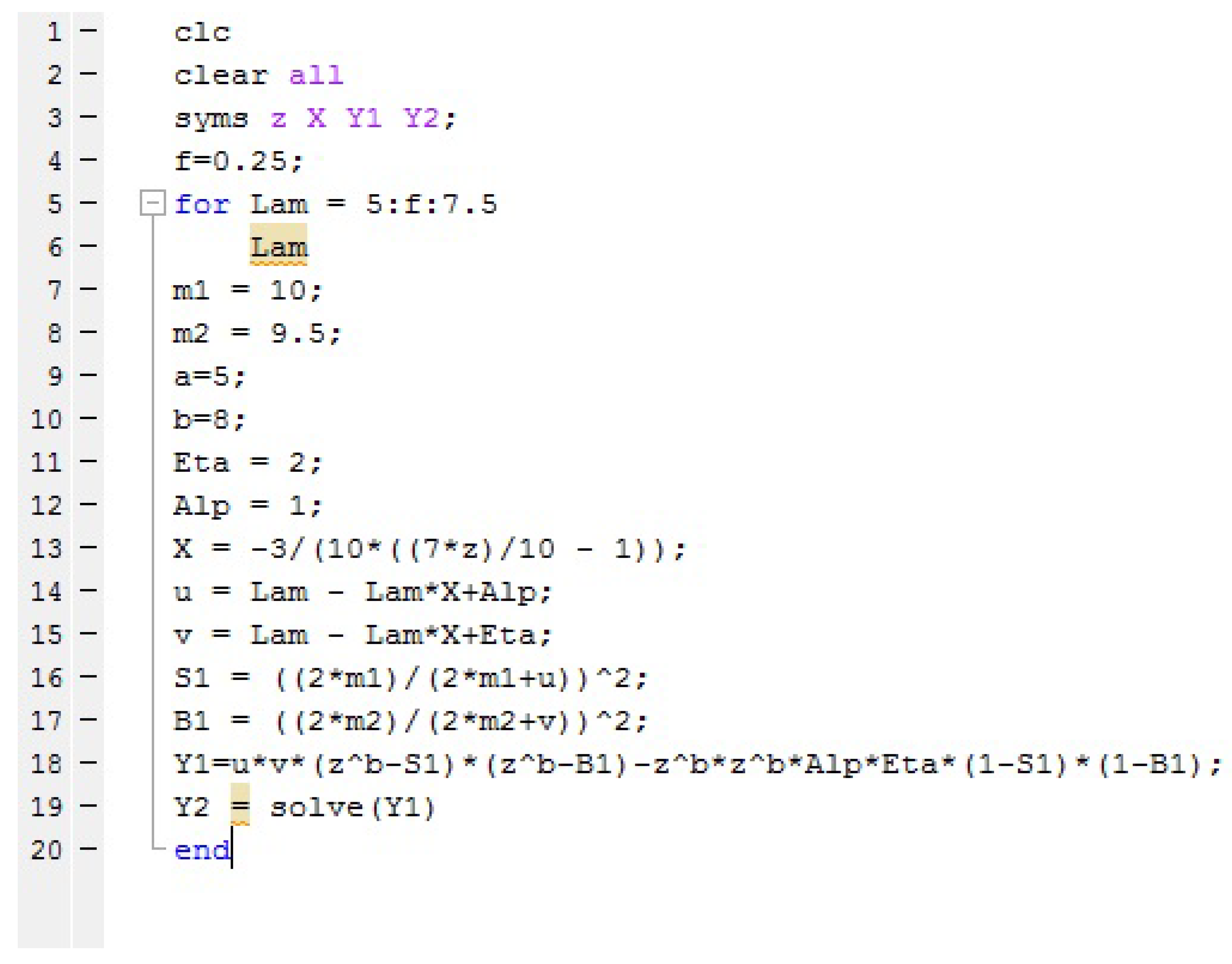
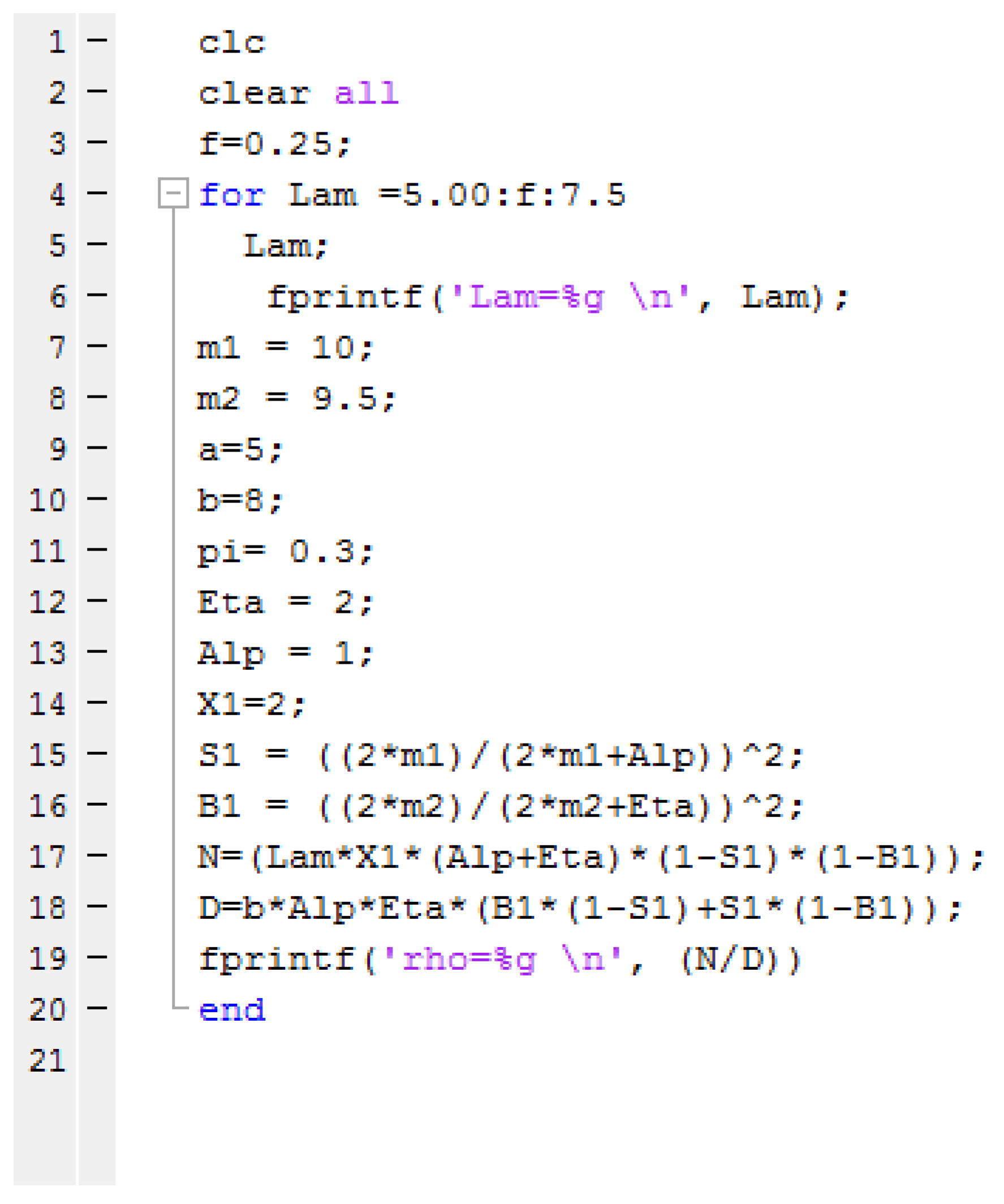
The unknown probabilities of the queue size distribution are computed using numerical techniques. The zeros of the function $Y_1\left(z\right)$ are obtained (see Figure 1) , and simultaneous equations are solved by using MATLAB. The values which are satisfies the stability condition (see Figure 2) are used for calculating the table values.

The expected queue length $E\left(Q\right)$ and the expected waiting time $E\left(W\right)$ are calculated for various arrival rate sand service rates, and the results are tabulated.

From

Table 1. Arrival rate vs. expected queue length and expected waiting time for the values $m_1=10,m_2=9.5,\alpha =1,\eta =2,\pi =0.3,ϵ=3,\mathrm{and}\omega =5$.

$\mathit{\lambda }$	$\mathit{\rho }$	$\mathit{E}\left(\mathit{Q}\right)$	$\mathit{E}\left(\mathit{W}\right)$
5.00	0.131407	8.657374	0.865737
5.25	0.137978	9.539724	0.908545
5.50	0.144548	10.375816	0.943256
5.75	0.151119	11.149076	0.969485
6.00	0.157689	11.843026	0.986919
6.25	0.164259	12.441064	0.995285
6.50	0.170830	12.927026	0.994387
6.75	0.177400	13.285663	0.984123
7.00	0.183970	13.502456	0.964461
7.25	0.190541	13.563622	0.935422
7.50	0.197111	13.456834	0.897122

,

Table 2. Main server’s service rate vs. expected queue length and expected waiting time for the values $\lambda =5,m_2=5,\alpha =1,\eta =2,$$\pi =0.3,ϵ=3,\mathrm{and}\omega =5$.

${\mathit{m}}_1$	$\mathit{\rho }$	$\mathit{E}\left(\mathit{Q}\right)$	$\mathit{E}\left(\mathit{W}\right)$
5.25	0.257410	26.824821	2.682482
5.50	0.248885	26.082729	2.608273
5.75	0.240905	25.388555	2.538855
6.00	0.233420	24.735574	2.473557
6.25	0.226385	24.117976	2.411798
6.50	0.219761	23.531054	2.353105
6.75	0.213513	22.971202	2.297120
7.00	0.207610	22.435611	2.243561
7.25	0.202024	21.921511	2.192151
7.50	0.196731	21.427009	2.142701
7.75	0.191707	20.950354	2.095035
8.00	0.186934	20.490051	2.049005

,

Table 3. Stand-by server’s service rate vs. expected queue length and expected waiting time for the values $\lambda =5,m_1=10,\alpha =1,\eta =2,$$\pi =0.3,ϵ=3,\mathrm{and}\omega =5$.

${\mathit{m}}_2$	$\mathit{\rho }$	$\mathit{E}\left(\mathit{Q}\right)$	$\mathit{E}\left(\mathit{W}\right)$
4.0	0.260103	65.007246	4.062953
4.5	0.254645	59.415276	3.713455
5.0	0.249401	53.808260	3.363016
5.5	0.244361	48.320593	3.020037
6.0	0.239515	43.028238	2.689265
6.5	0.234853	37.970425	2.373152
7.0	0.230366	33.162455	2.072653
7.5	0.226045	28.605406	1.787838
8.0	0.22188	24.292435	1.518277
8.5	0.217865	20.212075	1.263255
9.0	0.213991	16.351005	1.021938

and

Table 4. The effect of the main server’s vacation rate on expected queue length for the values

$\lambda =5,m_1=10,m_2=9.5,\alpha =1,\eta =2,\pi =0.3,\mathrm{and}ϵ=3$.

$\mathit{\omega }$	Erlang	Exponential
5.00	8.657374	8.279153
5.25	8.808004	8.448114
5.50	8.950939	8.607757
5.75	9.086640	8.758748
6.00	9.215535	8.901685
6.25	9.338068	9.037158
6.50	9.454625	9.165674
6.75	9.565595	9.287730
7.00	9.671330	9.403767
7.25	9.772165	9.514200
7.50	9.868410	9.619407
7.75	9.960351	9.719734
8.00	10.048247	9.815494

, the following observations can be made.

• As arrival rate $\lambda$ increases, the expected queue size and expected waiting time are also increase.
• When the main server’s and stand-by server’s service rate increases, the expected queue size and expected waiting time decrease.
• When the main server’s vacation rate increases, the expected queue size increases.

8. Conclusions

In this paper, a batch arrival general bulk service queueing system with breakdown and repair, stand-by server, multiple vacation and control policy on request for re-service is analyzed. The probability generating function of the queue size distribution at an arbitrary time is obtained. Some performance measures are calculated. The particular cases of the model are also deduced. From the numerical results, it is observed that when the arrival rate increases, the expected queue length and waiting time of the customers are also increase; if the service rate increases (for both server’s), then the expected queue length and expected waiting time decrease. It is also observed that, if the main server’s vacation rate increases, then the expected queue length increases.

References

- Doshi, B.T. Queueing systems with vacations—A survey. Queueing Syst. 1986, 1, 29–66. [Google Scholar] [CrossRef]
- Takagi, H. Vacation and Priority Systems. Queuing Analysis: A Foundation of Performance Evaluation; North-Holland: Amsterdam, The Netherlands, 1991; Volume I. [Google Scholar]
- Baba, Y. On the M[X]/G/1 queue with vacation time. Oper. Res. Lett. 1986, 5, 93–98. [Google Scholar] [CrossRef]
- Krishna Reddy, G.V.; Nadarajan, R.; Arumuganathan, R. Analysis of a bulk queue with N policy multiple vacations and setup times. Comput. Oper. Res. 1998, 25, 957–967. [Google Scholar] [CrossRef]
- Jeyakumar, S.; Senthilnathan, B. Modelling and analysis of a bulk service queueing model with multiple working vacations and server breakdown. RAIRO-Oper. Res. 2017, 51, 485–508. [Google Scholar] [CrossRef]
- Madan, K.C. An M/G/1 queue with second optional service. Queueing Syst. 2000, 34, 37–46. [Google Scholar] [CrossRef]
- Madan, K.C. On M[X]/(G1,G2)/1 queue with optional re-service. Appl. Math. Comput. 2004, 152, 71–88. [Google Scholar]
- Jeyakumar, S.; Arumuganathan, R. A Non-Markovian Bulk Queue with Multiple Vacations and Control Policy on Request for Re-Service. Qual. Technol. Quant. Manag. 2011, 8, 253–269. [Google Scholar] [CrossRef]
- Haridass, M.; Arumuganathan, R. A batch service queueing system with multiple vacations, setup time and server’s choice of admitting re-service. Int. J. Oper. Res. 2012, 14, 156–186. [Google Scholar] [CrossRef]
- Krishnamoorthy, A.; Pramod, P.K.; Chakravarthy, S.R. Queues with interruptions: A survey. Oper. Res. Decis. Theory 2014, 22, 290–320. [Google Scholar] [CrossRef]
- Ayyappan, G.; Shyamala, S. Transient solution of an M[X]/G/1 queueing model with feedback, random breakdowns, Bernoulli schedule server vacation and random setup time. Int. J. Oper. Res. 2016, 25, 196–211. [Google Scholar] [CrossRef]
- Choudhury, G.; Tadj, L. An M/G/1 queue with two phases of service subject to the server breakdown and delayed repair. Appl. Math. Model. 2009, 33, 2699–2709. [Google Scholar] [CrossRef]
- Senthilnathan, B.; Jeyakumar, S. A study on the behaviour of the server breakdown without interruption in a M[X]/G(a,b)/1 queueing system with multiple vacations and closedown time. Appl. Math. Comput. 2012, 219, 2618–2633. [Google Scholar]
- Lakshmi, K.; Kasturi Ramanath, K. An M/G/1 two phase multi-optional retrial queue with Bernoulli feedback, non-persistent customers and breakdown and repair. Int. J. Oper. Res. 2014, 19, 78–95. [Google Scholar] [CrossRef]
- Atencia, I. A discrete-time queueing system with server breakdowns and changes in the repair times. Ann. Oper. Res. 2015, 235, 37–49. [Google Scholar] [CrossRef]
- Choudhury, G. A batch arrival queue with a vacation time under single vacation policy. Comput. Oper. Res. 2002, 29, 1941–1955. [Google Scholar] [CrossRef]
- Jeyakumar, S.; Arumuganathan, R. Analysis of Single Server Retrial Queue with Batch Arrivals, Two Phases of Heterogeneous Service and Multiple Vacations with N-Policy. Int. J. Oper. Res. 2008, 5, 213–224. [Google Scholar]
- Balasubramanian, M.; Arumuganathan, R.; Senthil Vadivu, A. Steady state analysis of a non-Markovian bulk queueing system with overloading and multiple vacations. Int. J. Oper. Res. 2010, 9, 82–103. [Google Scholar] [CrossRef]
- Haridass, M.; Arumuganathan, R. Analysis of a batch arrival general bulk service queueing system with variant threshold policy for secondary jobs. Int. J. Math. Oper. Res. 2011, 3, 56–77. [Google Scholar] [CrossRef]
- Choudhury, G.; Deka, M. A batch arrival unreliable server delaying repair queue with two phases of service and Bernoulli vacation under multiple vacation policy. Qual. Technol. Quant. Manag. 2018, 15, 157–186. [Google Scholar] [CrossRef]
- Madan, K.C. A cyclic queueing system with three servers and optional two-way feedback. Microelectron. Reliabil. 1988, 28, 873–875. [Google Scholar] [CrossRef]
- Madan, K.C. On a single server queue with two-stage heterogeneous service and deterministic server vacations. Int. J. Syst. Sci. 2001, 32, 837–844. [Google Scholar] [CrossRef]
- Medhi, J. A Single Server Poisson Input Queue with a Second Optional Channel. Queueing Syst. 2002, 42, 239–242. [Google Scholar] [CrossRef]
- Arumuganathan, R.; Malliga, T.J. Analysis of a bulk queue with repair of service station and setup time. Int. J. Can. Appl. Math. Quart. 2006, 13, 19–42. [Google Scholar]
- Baruah, M.; Madan, K.C.; Eldabi, T. A Two Stage Batch Arrival Queue with Reneging during Vacation and Breakdown Periods. Am. J. Oper. Res. 2013, 3, 570–580. [Google Scholar] [CrossRef]
- Aissani, A.; Artalejo, J. On the single server retrial queue subject to breakdowns. Queueing Syst. 1988, 30, 309–321. [Google Scholar] [CrossRef]
- Maraghi, F.A.; Madan, K.C.; Darby-Dowman, K. Bernoulli schedule vacation queue with batch arrivals and random system breakdowns having general repair time distribution. Int. J. Oper. Res. 2010, 7, 240–256. [Google Scholar] [CrossRef]
- Fadhil, R.; Madan, K.C.; Lukas, A.C. An M(X)/G/1 Queue with Bernoulli Schedule General Vacation Times, Random Breakdowns, General Delay Times and General Repair Times. Appl. Math. Sci. 2011, 5, 35–51. [Google Scholar]
- Rajadurai, P.; Varalakshmi, M.; Saravanarajan, M.C.; Chandrasekaran, V.M. Analysis of M[X]/G/1 retrial queue with two phase service under Bernoulli vacation schedule and random breakdown. Int. J. Math. Oper. Res. 2015, 7, 19–41. [Google Scholar] [CrossRef]
- Jiang, T.; Xin, B. Computational analysis of the queue with working breakdowns and delaying repair under a Bernoulli-schedule-controlled policy. J. Commun. Stat. Theory Methods 2018, 1–16. [Google Scholar] [CrossRef]
- Madan, K.C. A bulk input queue with a stand-by. S. Afr. Stat. J. 1995, 29, 1–7. [Google Scholar]
- Khalaf, R.F. Queueing Systems With Four Different Main Server’s Interruptions and a Stand-By Server. Int. J. Oper. Res. 2014, 3, 49–54. [Google Scholar] [CrossRef]
- Jain, M.; Preeti. Cost analysis of a machine repair problem with standby, working vacation and server breakdown. Int. J. Math. Oper. Res. 2014, 6, 437–451. [Google Scholar] [CrossRef]
- Kumar, K.; Jain, M. Bi-level control of degraded machining system with two unreliable servers, multiple standbys, startup and vacation. Int. J. Oper. Res. 2014, 21, 123–142. [Google Scholar] [CrossRef]
- Murugeswari, N.; Maragatha Sundari, S. A Standby server bulk arrival Queuing model of Compulsory server Vacation. Int. J. Eng. Dev. Res. 2017, 5, 337–341. [Google Scholar]
- Kolledath, S.; Kumar, K.; Pippal, S. Survey on queueing models with standbys support. Yugoslav J. Oper. Res. 2018, 28, 3–20. [Google Scholar] [CrossRef]
- Neuts, M.F. A general class of bulk queues with poisson input. Ann. Math. Stat. 1967, 38, 759–770. [Google Scholar] [CrossRef]
- Ayyappan, G.; Sathiya, S. Non Markovian Queue with Two Types service Optional Re-service and General Vacation Distribution. Appl. Appl. Math. Int. J. 2016, 11, 504–526. [Google Scholar]
Figure 1.
MATLAB code for finding the roots.
Figure 2.
MATLAB code for finding the rho value.