Bifurcation Analysis of a Certain Hodgkin-Huxley Model Depending on Multiple Bifurcation Parameters

Abstract

In this paper, we study the dynamics of a certain Hodgkin-Huxley model describing the action potential (AP) of a cardiac muscle cell for a better understanding of the occurrence of a special type of cardiac arrhythmia, the so-called early afterdepolarisations (EADs). EADs are pathological voltage oscillations during the repolarisation or plateau phase of cardiac APs. They are considered as potential precursors to cardiac arrhythmia and are often associated with deficiencies in potassium currents or enhancements in the calcium or sodium currents, e.g., induced by ion channel diseases, drugs or stress. Our study is focused on the enhancement in the calcium current to identify regions, where EADs related to enhanced calcium current appear. To this aim, we study the dynamics of the model using bifurcation theory and numerical bifurcation analysis. Furthermore, we investigate the interaction of the potassium and calcium current. It turns out that a suitable increasing of the potassium current adjusted the EADs related to an enhanced calcium current. Thus, one can use our result to balance the EADs in the sense that an enhancement in the potassium currents may compensate the effect of enhanced calcium currents.

1. Introduction

The aim of this manuscript is the mathematical and numerical investigation of a three-dimensional Hodgkin-Huxley model from [1] to study early afterdepolarisations (EADs) in a cardiac muscle cell. Here, we are interested in the dynamics of this system and mainly in reasons for the occurrence of EADs. More precisely, we are interested in the sudden change from a normal action potential (AP) to this special type of cardiac arrhythmia. In general, EADs are additional small amplitude spikes during the plateau or the repolarisation phase of the AP. The presence of EADs strongly correlates with the onset of dangerous cardiac arrhythmias, including torsades de pointes (TdP), which is a specific type of abnormal heart rhythm that can lead to sudden cardiac death, see [2,3,4]. Please see for more (biological/physiological) details [5,6,7,8,9,10,11]. In this paper, we will use the bifurcation analysis similar to [12,13,14] to study the system introduced in [1]. We want to highlight that we can use our approach to investigate also more complex models, see for instance [15,16,17]. The numerical effort will be higher but we can use this basic principle for further studies. Moreover, our approach can be utilised to study the ion current interaction of all ion currents; this approach is not restricted to the investigation of the potassium–calcium current interaction. In addition, the general aim is to extend this research to models of the complete heart, cf. [18,19]. The main novelty of this paper is the consideration of a bifurcation problem depending on two bifurcation parameters to investigate the ion current interaction and the occurrence of EADs related to the calcium current. Furthermore, we want to mention that the intention of our manuscript is to present our results to a wide range of scientific researcher with different background in biology, mathematics, physics and physiology.

In last decades, the mathematical investigation of phenomena from life science, especially mathematical modelling and mathematical analysis, aroused more and more importance, as well as interdisciplinary research involving mathematics. A very important topic in recent years is the mathematical investigation of (human) diseases, e.g., tumor growth as well as diseases in neurons or cardiac muscle cells. Also here we have the aim to push forward this progress using our knowledge from mathematics to refine and extend existing theory and results. To this goal we choose the model from [1] for our study of EADs, where the authors studies two types of cardiac arrhythmias for instance EADs related to a deficit in the potassium current. Later we will give more details on their approach and how it differs from our ansatz, please see Section 3.2. In this paper, the authors chose the model from [20] and considered a modified reduced version, which they final reduced to a two-dimensional model (fast subsystem) for their investigation. Using their approach the authors in [1] have shown that EADs can occur during the transition between stable steady states. Moreover, they argued their study shows that a stable limit cycle in the fast subsystem is not required for EAD generation. In Section 3.2, we will explain and show why this approach is not applicable to study and to understand EADs related to an enhancement in the calcium current.

Moreover, there are several cardiac cell models available, e.g., the famous Luo-Rudy model [17] describing a cardiac muscle cell of guinea pigs. Furthermore, we want to refer to the review article on cardiac cell modelling [16], where the authors give a nice overview on existing cardiac cell models, as well as to the review article on cardiac tissue modelling [15].

In addition to the modelling of phenomena in the real life it is very important to analyse the behaviour of the corresponding model and to study its dynamics. To this aim we are using the bifurcation theory, since this theory provides a strategy for investigating the bifurcations and the behaviour of the system, please see Section 3. Furthermore, we want to highlight the monographs [12,13,14]. These monographs give a very good introduction and nice overview on this topic. In [12] the author does not only explain and discuss the bifurcation theory, he also provides the numerical background for the numerical bifurcation analysis. Moreover, the books [13,14] are focused on the qualitative study of high-dimensional nonlinear dynamical systems and chaos. Beside these books there are plenty of further good books dealing with the topics of dynamical systems, bifurcations and chaos, but we cannot cite them all in this manuscript.

The paper is organised as follows. First of all in Section 2, we will give a brief introduction into the topic of cardiac APs and arrhythmia, i.e., afterdepolarisations. Then, we will go on with the mathematical modelling of the cardiac AP using a Hodgkin-Huxley type formalism, which is the usual approach for the modelling of AP for neurons and cardiac muscle cells. In Section 3 and Section 4, we will explain the behaviour of the considered model using the bifurcation analysis. The desired bifurcation diagram we will derive utilising MATLAB together with the toolboxes MATCONT and CL_MATCONT [21,22,23], which are numerical continuation packages for the interactive bifurcation analysis of dynamical systems. In Section 5, we show how we can compensate or control the occurrence of EADs. Finally, we will finish this paper with a discussion.

2. Biological Background and Mathematical Modelling

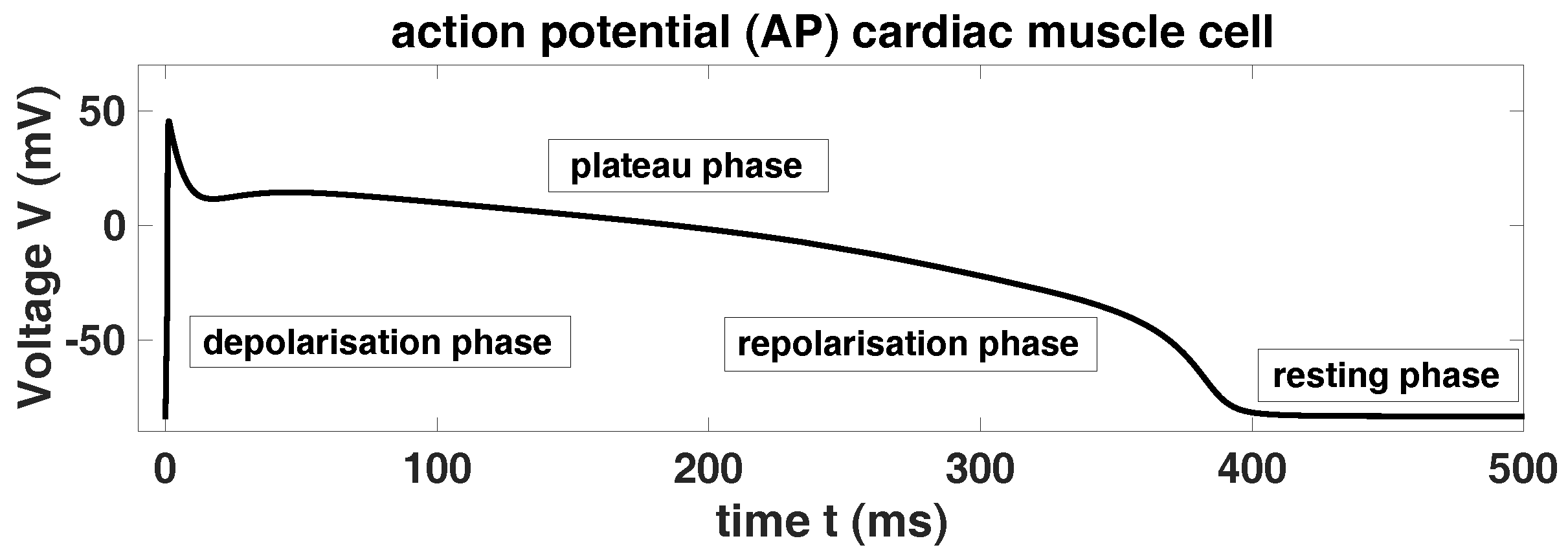
Action potential. An AP is a temporary, characteristic variance of the membrane potential of an excitable biological cell, e.g., neuron or cardiac muscle cell, from its resting potential. The molecular mechanism of an AP is based on the interaction of voltage-sensitive ion channels. The reason for the formation and the special properties of the AP is established in the properties of different groups of ion channels in the plasma membrane. An initial stimulus activates the ion channels as soon as a certain threshold potential is reached. Then, these ion channels break open and/or up such that this interaction allows an ion current, which changes the membrane potential. A normal AP is always uniform and the cardiac muscle cell AP is typically divided in four phases, i.e., the resting phase, the upstroke phase, the (long) plateau phase and the repolarisation phase, see Figure 1:

The resting phase/potential is designated by high potassium (K${}^{+}$) currents, while after the initial stimulus the sodium (Na${}^{+}$) conductance increases rapidly and the Na${}^{+}$ current flux into the cardiac muscle cell until a spike potential (ca. +30 mV) is achieved. This spike potential is the so-called upstroke or overshot. Then, the Na${}^{+}$ current inactivates rapidly followed by the activation of L-type calcium (Ca${}^{2+}$) current. The Ca${}^{2+}$ current is more slowly than the Na${}^{+}$ current and plays a key role in maintaining the long plateau phase, which is characteristic for the cardiac muscle cell. The overall duration of this long AP is at 220–400 ms. Moreover, while the Ca${}^{2+}$ conductance increases the K${}^{+}$ conductance decreases. The plateau phase is followed by the repolarisation phase, where the intrinsic K${}^{+}$ ion channels are activated and this is connected with the reduction of the Ca${}^{2+}$ conductance. Finally, the K${}^{+}$ current increases until the resting potential respectively the resting phase is reached. In contrast to the Na${}^{+}$ and Ca${}^{2+}$ currents is the K${}^{+}$ current an outward current.

Afterdepolarisation. If there are depolarising variations of the membrane voltage, then we are speaking about afterdepolarisations. These afterdepolarisations are divided in early afterde-polarisations (EADs) and delayed afterdepolarisations (DADs). This division depends on the timing obtaining of the AP. EADs occur either in the plateau or the repolarisation phase of the AP. EADs are benefited by an elongation of the AP, while the DADs occur after the repolarisation phase is completed. EADs are additional small amplitude spikes during the plateau or the repolarisation phase of the AP, cf. Figure 2.

They are resulting, e.g., from a reduction of the repolarising K${}^{+}$ currents or from an intensification of depolarising Na${}^{+}$ currents or Ca${}^{2+}$ currents. Triggers for this are congenital disorders of the ion channels (congenital Long- QT-Syndrome) or the ingestion of some medicaments. The elongation of the AP could generate afterpolarisations by reactivation L-type Ca${}^{2+}$ influx. Also chronic cardiac insufficiency could appear with an elongation of the AP by a reduction of the repolarising K${}^{+}$ currents. This means, EADs are often associated with deficits in the potassium currents or enhancements in the calcium currents.

The model. In general, APs of excitable biological cells such as neurons and cardiac muscle cells are often modelled as an ODE system using a Hodgkin-Huxley type formalism, please see the paper of Hodgkin and Huxley [24] and the book of Izhikevich [25]. In this paper, we will study the model from [1]—a toy model—which depends only on two ion currents, the potassium (K${}^{+}$) current and the calcium (Ca${}^{2+}$) current, as a simplification for the study of EADs. Please notice that in this model the sodium current is not considered. Furthermore, the system is self-oscillating, which means that we do not need an initial stimulus. Nevertheless, this is a suitable starting point for the study of EADs, since EADs appear either in the plateau or the repolarisation phase. Here, the potassium (K${}^{+}$) and the calcium (Ca${}^{2+}$) currents are important, see [1,26]. The model is a three-dimensional ODE system, which contains the potassium current $I_K=G_{\mathrm{K}}·x·(V-E_{\mathrm{K}})$ and the calcium current $I_{\mathrm{Ca}}=G_{\mathrm{Ca}}·f·d_{\infty }\left(V\right)·(V-E_{\mathrm{Ca}})$, where V denotes the membrane voltage, $d_{\infty }\left(V\right)$ is the steady state of the gating variable d given in (2), $G_{\mathrm{K}}=0.05\frac{\mathrm{mS}}{{\mathrm{cm}}^2}$ and $G_{\mathrm{Ca}}=0.025\frac{\mathrm{mS}}{{\mathrm{cm}}^2}$ denote the ion current conductances, while x and f represent the gating variables, which are important for the opening and closing of the different ion channels. Moreover, $E_{\mathrm{K}}$ and $E_{\mathrm{Ca}}$ denote the Nernst potential of the ion currents, cf.

Table 1. System parameters of model (1).

Abbr.	Value	Unit	Abbr.	Value	Unit	Abbr.	Value	Unit
$V_{T_d}$	−35.0	mV	$k_d$	−6.24	mV	$E_{\mathrm{K}}$	−80.0	mV
$V_{T_f}$	−20.0	mV	$k_f$	8.6	mV	$E_{\mathrm{Ca}}$	100.0	mV
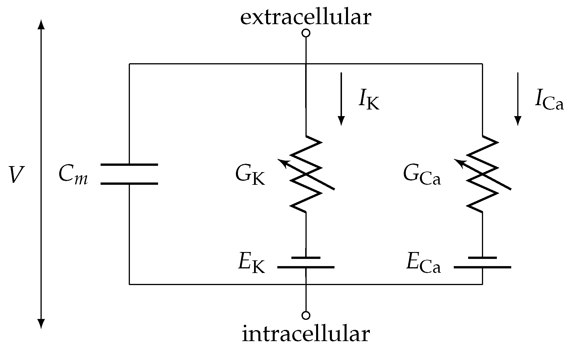
$V_{T_x}$	−40.0	mV	$k_x$	−5	mV	V	(−80; 100)	mV

. The physical system (Figure 3) one has in mind is the following

and the corresponding mathematical model read as follows:

$$\begin{array}{c}\hfill \left\{\begin{array}{cc}{\displaystyle \frac{\mathrm{d}V}{\mathrm{d}t}}\hfill & {\displaystyle =-\frac{I_{\mathrm{K}}+I_{\mathrm{Ca}}}{C_m}=:F_1(V,f,x),}\hfill \\ {\displaystyle \frac{\mathrm{d}f}{\mathrm{d}t}}\hfill & {\displaystyle =\frac{f_{\infty }\left(V\right)-f}{{\tau }_f}=:F_2(V,f,x),}\hfill \\ {\displaystyle \frac{\mathrm{d}x}{\mathrm{d}t}}\hfill & {\displaystyle =\frac{x_{\infty }\left(V\right)-x}{{\tau }_x}=:F_3(V,f,x),}\hfill \end{array}\right.\end{array}$$

(1)

where ${\tau }_f=80$ ms and ${\tau }_x=300$ ms denote the relaxation time constant of the corresponding channel gating variables. Further, the membrane capacitance is given by $C_m=1\mathsf{\mu }$F/cm${}^2$, cf. [1,20,27]. As we already mentioned, the gating variables are important for the opening and closing of the different ion channels. This means (for instance explained for $I_K$ and $x\in [0,1]$) that if $x=0$ the potassium channel is closed, i.e., there is no potassium current flow ($I_K=0$), while if $x=1$ the potassium channel is complete open. We have also to mention that the calcium current is depending on a second gating variable d, which is assumed to be equal to its equilibrium, cf. (2).

Conductance-based models are based on an equivalent circuit representation of a cell membrane. These models represent a minimal biophysical interpretation for an excitable biological cell in which current flow across the membrane is due to charging of the membrane capacitance and movement of ions across ion channels. Ion channels are selective for particular ionic species, such as calcium or potassium, giving rise to currents $I_{\mathrm{Ca}}$ or $I_{\mathrm{K}}$, respectively. In addition, the equilibria of the gating variables are represented by

$$\begin{array}{c}\hfill y_{\infty }\left(V\right):={\left(1+exp\left(\frac{V-V_{T_y}}{k_y}\right)\right)}^{-1},\end{array}$$

(2)

where y represents the gating variables d, f and x we will use the abbreviations $y_{\infty }:=y_{\infty }\left(V\right)$ with

In this setting there are no EADs, but it is well known that the reduction of the potassium or the enhancements in the calcium current or a combination of both may yield EADs. In this manuscript we are focused on the enhancements in the $I_{\mathrm{Ca}}$ current and the resulting behaviour of system (1).

3. Bifurcation Theory

A bifurcation of a dynamical system is a qualitative change in its dynamics produced by varying parameters. We consider an autonomous system of ordinary differential equations, where the right hand side of this system is depending on several state variables and parameter(s), cf. system (1). V, f and x denote the state variables, while $G_{\mathrm{K}}$ and $G_{\mathrm{Ca}}$ are the parameters of our interest. Since we study the occurrence of EADs induced by an enhancement in the calcium current $I_{\mathrm{Ca}}$, we will choose the conductance $G_{\mathrm{Ca}}$ as the bifurcation parameter to be able to simulate the decreasing or mainly the increasing of the current $I_{\mathrm{Ca}}$. In general, a bifurcation occurs at some parameter p (in our case $G_{\mathrm{Ca}}$), if there are parameter values arbitrarily close to p with dynamics topologically inequivalent from those at p. For example, an equilibrium of the considered system may lose or win stability at a bifurcation, or a limit cycle may occur. The bifurcation theory provides a strategy for investigating the bifurcations and the behaviour of the system. This basic idea we will use to study the dynamics of (1) and the reasons for the appearing of EADs. Therefore, we choose the conductance $G_{\mathrm{Ca}}$ as bifurcation parameter and we start determining the equilibrium of model (1). This yields $f\equiv f_{\infty }\left(V\right)$ and $x\equiv x_{\infty }\left(V\right)$. Moreover, we have the following condition for the equilibrium of the voltage V:

$$\begin{array}{c}\hfill -G_{\mathrm{K}}·x_{\infty }\left(V\right)·(V-E_{\mathrm{K}})-G_{\mathrm{Ca}}·f_{\infty }\left(V\right)·d_{\infty }\left(V\right)·(V-E_{\mathrm{Ca}})=0.\end{array}$$

(3)

Please note that in system (1) we have at least four system parameters, which are important for the behaviour of the system, i.e., $G_{\mathrm{Ca}}$, $G_{\mathrm{K}}$, ${\tau }_f$ and ${\tau }_x$. Here, we are focused mainly on the dependences on $G_{\mathrm{Ca}}$ but also on $G_{\mathrm{K}}$. Further, we want to emphasise, if we change ${\tau }_f$ and/or ${\tau }_x$, then this has also an effect on the behaviour of the model (1).

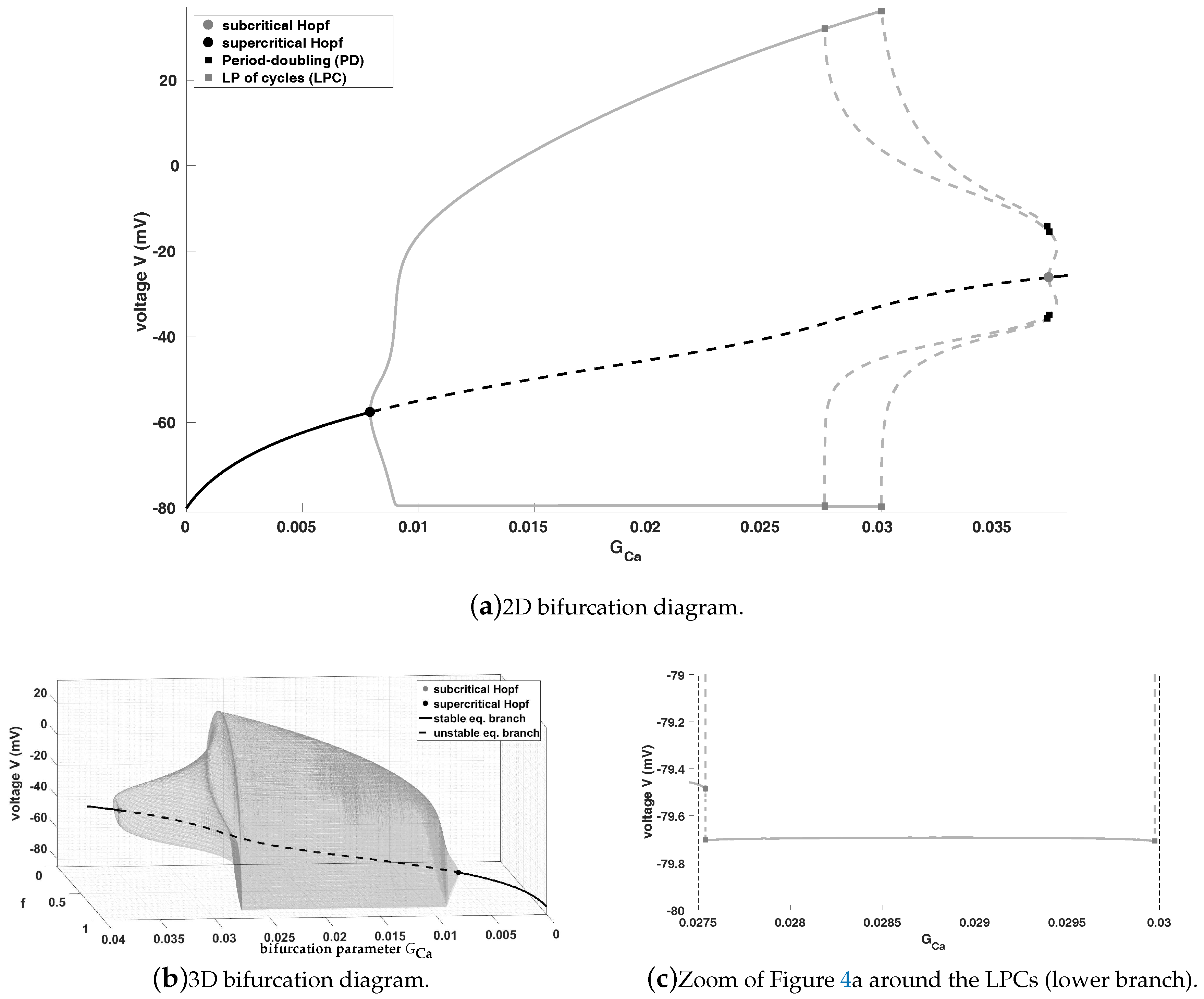
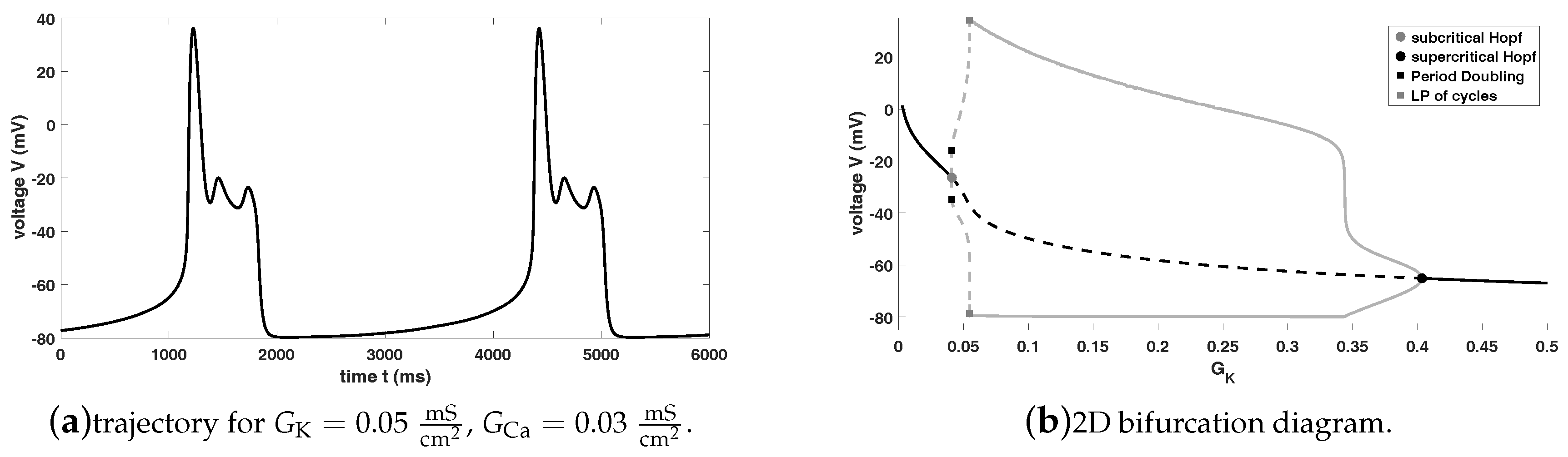
At this stage, we see—cf. condition (3)—that the choice of $G_{\mathrm{Ca}}$ has a direct influence on the location of the equilibrium and its stability (considering the corresponding eigenvalues). Therefore, varying the bifurcation parameter $G_{\mathrm{Ca}}$ yields different equilibria with probably different stability. Figure 4 shows the bifurcation diagram of system (1), where we use $G_{\mathrm{Ca}}$ as the bifurcation parameter for fixed $G_{\mathrm{K}}=0.05\frac{\mathrm{mS}}{{\mathrm{cm}}^2}$. For our bifurcation analysis and the calculation of our bifurcation diagram we are using MATCONT in combination with MATLAB. Please notice that all figures are produced using MATLAB. Figure 4a shows the bifurcation diagram ($G_{\mathrm{Ca}},V$) with two limit cycle branches, while Figure 4b shows the bifurcation diagram ($G_{\mathrm{Ca}},f,V$) with (only) the first limit cycle branch. Furthermore, in Figure 4c we state the zoom of Figure 4a around the LPCs (lower limit cycle branches) including two vertical dashed lines for an easier comprehension.

This bifurcation diagram shows that the equilibrium curve loses stability via a subcritical Andronov-Hopf bifurcation (grey dot) and wins stability via a supercritical Andronov-Hopf bifurcation (black dot)—Figure 4a from right to left and Figure 4b from left to right. Moreover, an unstable limit cycle branch bifurcates from the subcritical Andronov-Hopf bifurcation (positive first Lyapunov coefficient), which becomes stable via a limit point bifurcation (LP) of cycles (also known as fold or saddle-node bifurcation of cycles, which generically corresponds to a turning point of a curve of limit cycles) and finally, disappears via the supercritical Andronov-Hopf bifurcation (negative first Lyapunov coefficient). Please notice that after the supercritical Andronov-Hopf bifurcation the steady state becomes an unstable saddle-focus for $G_{\mathrm{Ca}}$ values approximately between $(0.080;0.0138)$. For values approximately between $(0.0138;0.0320)$ it turns into a saddle before it becomes again an unstable saddle-focus and gains again stability via the subcritical Andronov-Hopf bifurcation. Please note that the saddle has always two positive and one negative (real) eigenvalue, i.e., we have a two-dimensional unstable and an one-dimensional stable manifold. From this bifurcation diagram it is obvious that oscillations (in the sense of periodic orbits, which are not converging into an equilibrium or which no more reach the resting potential) can occur only between the two Andronov-Hopf bifurcations—also trajectories, which are not related to EADs. Notice that the system (1) exhibits also oscillations for values of $G_{\mathrm{Ca}}$ close to the right hand side of the subcritical Andronov-Hopf bifurcation, but the trajectory will either converge into a stable focus after a certain amount of time, which would be related to the sudden death if this behaviour spread over the heart, or oscillations occur, which exhibit no resting phase and oscillate continuously (depending on the initial values). Since the aim of this paper is to identify the region, where EADs appear, to be able to control them and to prevent the sudden death, we are focused on the distinction of the spiking regions (related to normal AP) and the bursting region (with periodic orbits related to EADs). However, EADs are in general complex oscillatory phenomena and could have one or more additional small oscillations. For simplicity we will analyse and point out, where system (1) have no additional small oscillations and for which values of $G_{\mathrm{Ca}}$ EADs appear.

At this stage, we have to notice that increasing of $G_{\mathrm{Ca}}$ and therefore, increasing of the calcium current $I_{\mathrm{Ca}}$ may yields EADs, which was expected. Moreover, this bifurcation diagram implies that EADs can appear only for values of $G_{\mathrm{Ca}}$ between the subcritical Andronov-Hopf bifurcation ($G_{\mathrm{Ca}}\approx 0.0372\frac{\mathrm{mS}}{{\mathrm{cm}}^2}$) and LP of cycles ($G_{\mathrm{Ca}}\approx 0.0275\frac{\mathrm{mS}}{{\mathrm{cm}}^2}$), which is the separatrix between EADs and no EADs, since “after” the first LP of cycles there are no additional small oscillations. From this LP of cycles we have the stable limit cycle branch, while from the first period doubling bifurcation again an unstable limit cycle branch bifurcates, which becomes stable after a further LP of cycles, again unstable via a third LP of cycles before this branch converges into the first unstable limit cycle branch. 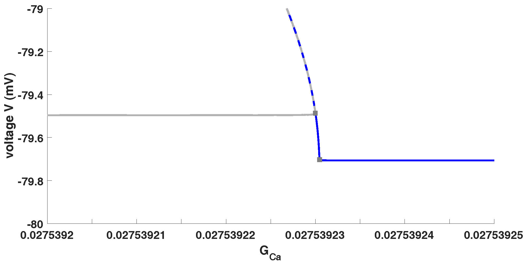Please notice that we do not have isolas as in [28] but we also have a similar splitting into a spiking and a bursting region, see Figure 4c and its refined view in Figure 5.

In Figure 5 we plot the continuation from the first PD (the second limit cycle branch) as a solid blue line to illustrate in a better way the situation we mentioned above. Furthermore, we want to highlight that such models (which exhibit one or more PD) might exhibit isolas as in [28] or a PD cascade as in [27]. In the case that there exists a (stable) PD cascade then the model contains chaos depending on the value of the bifurcation parameter. This is depending on the choices of the system parameters, e.g., ${\tau }_f$ and ${\tau }_x$. However, the (unforced) system (1) exhibits no chaotic pattern or trajectories. But, chaotic trajectories may occur for different values of ${\tau }_f$ and ${\tau }_x$. Please see for more details [27], where we have shown that system (1) may have a (stable) PD cascade, which is usually the route to chaos.

3.1. Bifurcation Analysis with $G_{\mathrm{K}}$ as Bifurcation Parameter

Our next observation is, if we choose $G_{\mathrm{Ca}}=0.03\frac{\mathrm{mS}}{{\mathrm{cm}}^2}$ and $G_{\mathrm{K}}=0.05\frac{\mathrm{mS}}{{\mathrm{cm}}^2}$, since we know from Figure 4c that we have two small oscillations (second LPC at $G_{\mathrm{Ca}}\approx 0.029976\frac{\mathrm{mS}}{{\mathrm{cm}}^2}$), i.e, an EAD—cf. Figure 6a—and we use now $G_{\mathrm{K}}$ as bifurcation parameter with fixed $G_{\mathrm{Ca}}=0.03\frac{\mathrm{mS}}{{\mathrm{cm}}^2}$, it turns out that increasing of the potassium current can balance the effect of an enhanced calcium current. From the bifurcation diagram in Figure 6b, we get that there are no EADs for $G_{\mathrm{Ca}}=0.03\frac{\mathrm{mS}}{{\mathrm{cm}}^2}$ and $G_{\mathrm{K}}$ values greater than $G_{\mathrm{K}}\approx 0.0548\frac{\mathrm{mS}}{{\mathrm{cm}}^2}$ (LP of cycles), while for values between $G_{\mathrm{K}}\approx 0.0408\frac{\mathrm{mS}}{{\mathrm{cm}}^2}$ (subcritical Andronov-Hopf bifurcation) and $G_{\mathrm{K}}\approx 0.0548\frac{\mathrm{mS}}{{\mathrm{cm}}^2}$ there are EADs, similar to the discussion from above. Therefore, the effect of an enhanced calcium current $I_{\mathrm{Ca}}$ can be compensated by an increasing of the potassium current $I_{\mathrm{K}}$.

Regarding Figure 6b, we see that if we choose a $G_{\mathrm{K}}$ value too close to the supercritical Andronov-Hopf bifurcation, then the voltage does not reach the resting potential. This indicates that we have normal AP as long as we choose a $G_{\mathrm{K}}$ value such that this value is greater than the value of the LP of cycles and the lower branch of the limit cycle branch is equal to the resting potential of the voltage.

3.2. Multiple Time Scales

Here, we want to remark that for instance in [1,26] the occurrence of EADs via the reduction of the potassium current is studied. The authors used a time scale separation argument (not explicit) to identify the gating variable x as the slowest variable and then, they argued in principle that EADs are Hopf-induced, cf. [29,30,31], by considering a fast subsystem using x as bifurcation parameter. This approach is not applicable in our situation, since the gating variable f is much faster than x. This one can realise since ${\tau }_f\ll {\tau }_x$, but we can show this also by the following time scale separation argument. To this aim we introduce a new (dimensionless) time variable $\tau$ satisfying $t:=k_t·\tau$, where $k_t$ is a reference time we have to choose. Choosing $k_t={\tau }_x$ and re-writing system (1) we get:

$$\begin{array}{c}\hfill \left\{\begin{array}{cc}{\displaystyle \epsilon \frac{\mathrm{d}V}{\mathrm{d}\tau }}\hfill & =-(I_{\mathrm{K}}+I_{\mathrm{Ca}}),\hfill \\ {\displaystyle \delta \frac{\mathrm{d}f}{\mathrm{d}\tau }}\hfill & =(f_{\infty }\left(V\right)-f),\hfill \\ \hfill {\displaystyle \frac{\mathrm{d}x}{\mathrm{d}\tau }}& =(x_{\infty }\left(V\right)-x),\hfill \end{array}\right.\end{array}$$

(4)

where we divided also the first equation by $G:=max\left\{G_{\mathrm{K}},G_{\mathrm{Ca}}\right\}$ and defined ${\overline{G}}_{\mathrm{K}}:=\frac{G_{\mathrm{K}}}{G}$ and ${\overline{G}}_{\mathrm{Ca}}:=\frac{G_{\mathrm{Ca}}}{G}$ to derive the dimensionless singular perturbation parameters $\epsilon :=\frac{C_m}{{\tau }_x·G}$ and $\delta :=\frac{{\tau }_f}{{\tau }_x}$. Please note that we chose as reference time $k_t$ the maximum of all relaxation time constants. Using the setting from above we have that $0\le \epsilon <\delta \ll 1$, i.e., three different time scales. Furthermore, we want to highlight that also different choices of the singular perturbation parameters yield that the gating variable x is always the slowest variable and the corresponding fast subsystem is either 1 dimensional (if $\epsilon \to 0$ and $\delta \ne 0$ fixed), i.e., it cannot exhibit an Andronov-Hopf bifurcation, or 2 dimensional (if $\delta \equiv \epsilon$, $\epsilon \to 0$):

$$\begin{array}{c}\hfill \left\{\begin{array}{cc}\hfill {\displaystyle \frac{\mathrm{d}V}{\mathrm{d}{\tau }_{\mathrm{fast}}}}& =-(I_{\mathrm{K}}+I_{\mathrm{Ca}}),\hfill \\ \hfill {\displaystyle \frac{\mathrm{d}f}{\mathrm{d}{\tau }_{\mathrm{fast}}}}& {\displaystyle =\frac{G}{{\tau }_f{C}_m}(f_{\infty }\left(V\right)-f),}\hfill \\ \hfill x& =\mathrm{const}.,\hfill \end{array}\right.\end{array}$$

where we rescaled in time, i.e., ${\tau }_{\mathrm{fast}}=\tau /\epsilon$, and considered the singular limit ${\tau }_x\to \infty$ yielding $\epsilon \to 0$. Therefore, EADs appearing in system (1) via an enhanced calcium current are not Hopf-induced in the sense of geometric singular perturbation theory, please see the book of Kuehn [31] for more details. Again, we want to highlight that EADs may occur as Hopf-induced mixed mode oscillations via a reduction of the potassium current, but not via an enhancement in the calcium current.

4. Two bifurcation problem

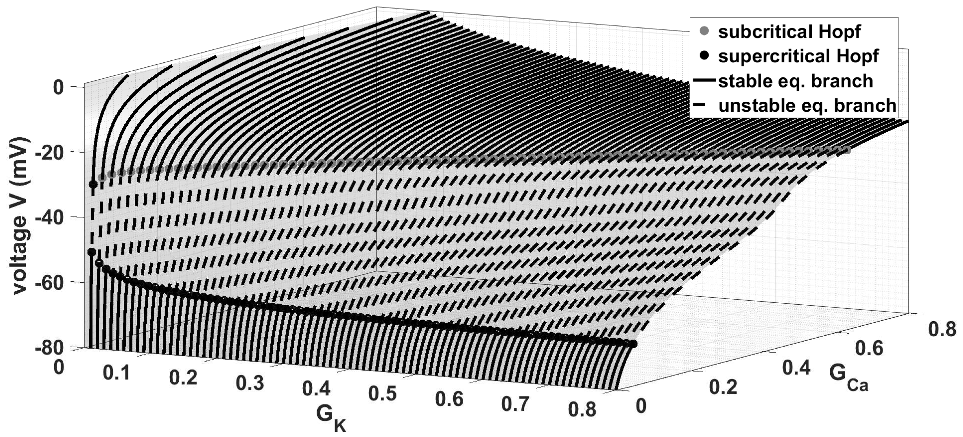
Our next aim is to use the previous result to investigate the ion current interactions by considering a two bifurcation problems. First of all, we have to notice that varying simultaneous the conductances $G_{\mathrm{K}}$ and $G_{\mathrm{Ca}}$ yields the equilibrium curves in Figure 7. For suitable values of $G_{\mathrm{K}}$ and $G_{\mathrm{Ca}}$ the stable equilibrium branch loses stability via an Andronov-Hopf bifurcation (sub- or supercritical) and becomes stable via a further (supercritical) Andronov-Hopf bifurcation. The range, where system (1) oscillates, increases for increased values of $G_{\mathrm{K}}$ and $G_{\mathrm{Ca}}$.

This has also a huge influence on the behaviour of the complete system. Moreover, for each new limit cycle branch the trajectory has a further small oscillation (via a PD cascade or isolas), depending on the choice of $G_{\mathrm{Ca}}$. This means—cf. Figure 4—that the trajectory has one small oscillation for $G_{\mathrm{Ca}}$ values approximately between $[0.02754;0.02997]$. At this stage, we emphasise that our approach can be extended to a multiple bifurcation problem of system (1) with up to five main important parameters, i.e., $G_{\mathrm{K}}$, $G_{\mathrm{Ca}}$, $C_m$, ${\tau }_f$ and ${\tau }_x$. 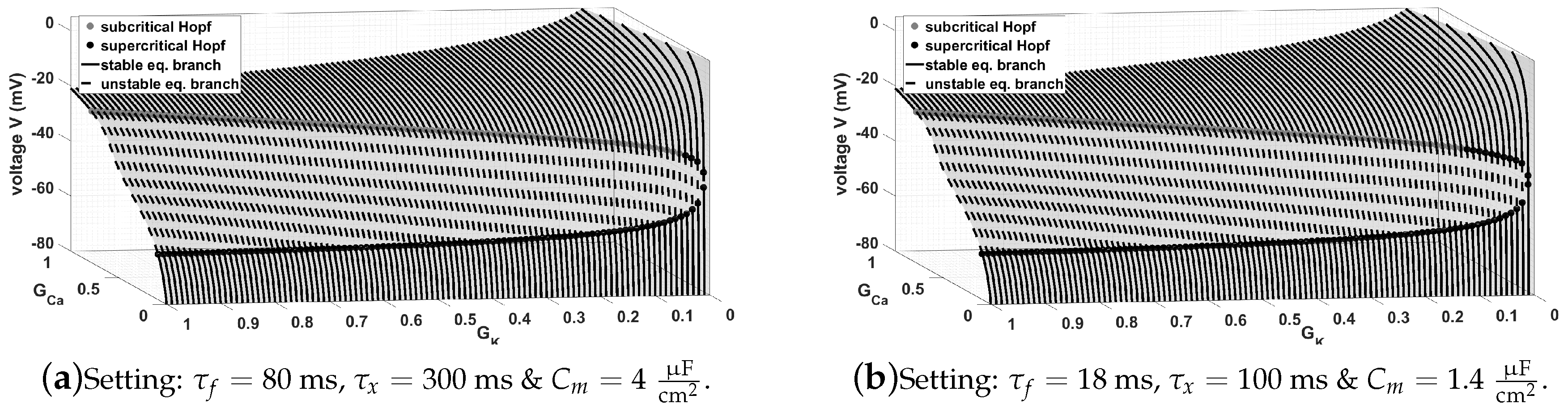While the shape of the equilibrium curves are depending on $G_{\mathrm{K}}$ and $G_{\mathrm{Ca}}$, the shape of the equilibrium curves remain the same by varying $C_m$, ${\tau }_f$ or ${\tau }_x$, but the behaviour is depending on these parameters, cf. Figure 8. Moreover, the Andronov-Hopf bifurcations in Figure 7 and Figure 8 form two “Hopf-curves”, which continuously depend on $G_{\mathrm{K}}$ and $G_{\mathrm{Ca}}$. This we can also prove by the Routh-Hurwitz criterion, see [13]. For this aim we determine the characteristic equation

$$\begin{array}{c}\hfill -det(A-\lambda {𝟙}_3)={\lambda }^3+a_1{\lambda }^2+a_2\lambda +a_3=0,\end{array}$$

(5)

where A denotes the Jacobian of system (1) evaluated at the equilibrium of system (1). The Routh-Hurwitz criterion implies that all characteristic exponents of Equation (5) have negative real parts if and only if the conditions

$$\begin{array}{c}\hfill {\Delta }_1=a_1>0,{\Delta }_2=a_1{a}_2-a_3>0\mathrm{and}{\Delta }_3=a_3(a_1{a}_2-a_3)>0\end{array}$$

are satisfied, which implies that the equilibrium is asymptotically stable, where $a_1=\left(\frac{1}{{\tau }_f}+\frac{1}{{\tau }_x}-\frac{\partial F_1}{\partial V}\right)$, $a_2=\left(\frac{1}{{\tau }_f{\tau }_x}-\left(\frac{1}{{\tau }_f}+\frac{1}{{\tau }_x}\right)\frac{\partial F_1}{\partial V}-\frac{1}{{\tau }_f}\frac{\partial f_{\infty }}{\partial V}\frac{\partial F_1}{\partial f}-\frac{1}{{\tau }_x}\frac{\partial x_{\infty }}{\partial V}\frac{\partial F_1}{\partial x}\right),$ $a_3=-\frac{1}{{\tau }_f{\tau }_x}\left(\frac{\partial x_{\infty }}{\partial V}\frac{\partial F_1}{\partial x}+\frac{\partial f_{\infty }}{\partial V}\frac{\partial F_1}{\partial f}+\frac{\partial F_1}{\partial V}\right)$ and

$$\begin{array}{cc}\hfill {\Delta }_2& =\frac{1}{{\tau }_f}\left(\frac{1}{{\tau }_f}-\frac{\partial F_1}{\partial V}\right)\left(\frac{1}{{\tau }_x}-\frac{\partial F_1}{\partial V}-\frac{\partial f_{\infty }}{\partial V}\frac{\partial F_1}{\partial f}\right)+\frac{1}{{\tau }_x}\left(\frac{1}{{\tau }_x}-\frac{\partial F_1}{\partial V}\right)\left(\frac{1}{{\tau }_f}-\frac{\partial F_1}{\partial V}-\frac{\partial x_{\infty }}{\partial V}\frac{\partial F_1}{\partial x}\right).\hfill \end{array}$$

Moreover, if ${\Delta }_1>0$, ${\Delta }_2=0$ and $a_3>0$ the equilibrium of system (1) is an Andronov-Hopf bifurcation with ${\lambda }_{1,2}=\pm \mathbf{i}{\omega }_0$, where ${\omega }_0^2=a_2>0$ and ${\lambda }_3=-a_1$, since

$$\begin{array}{c}\hfill {\lambda }^3+a_1{\lambda }^2+a_2\lambda +a_3={\lambda }_3+a_1{\lambda }^2+a_2\lambda +a_1{a}_2=({\lambda }^2+a_2)(\lambda +a_1)=0,\end{array}$$

where we used ${\Delta }_2=0$, cf. [14]. Furthermore, $a_1>0$ implies that ${\lambda }_3$ is negative. Especially, if ${\Delta }_2<0$ oscillations occur, which implies that $X\left(t\right)-X(t+T)=0$, where $X=\left\{V,f,x\right\}$ and T denotes the period of the periodic orbit. 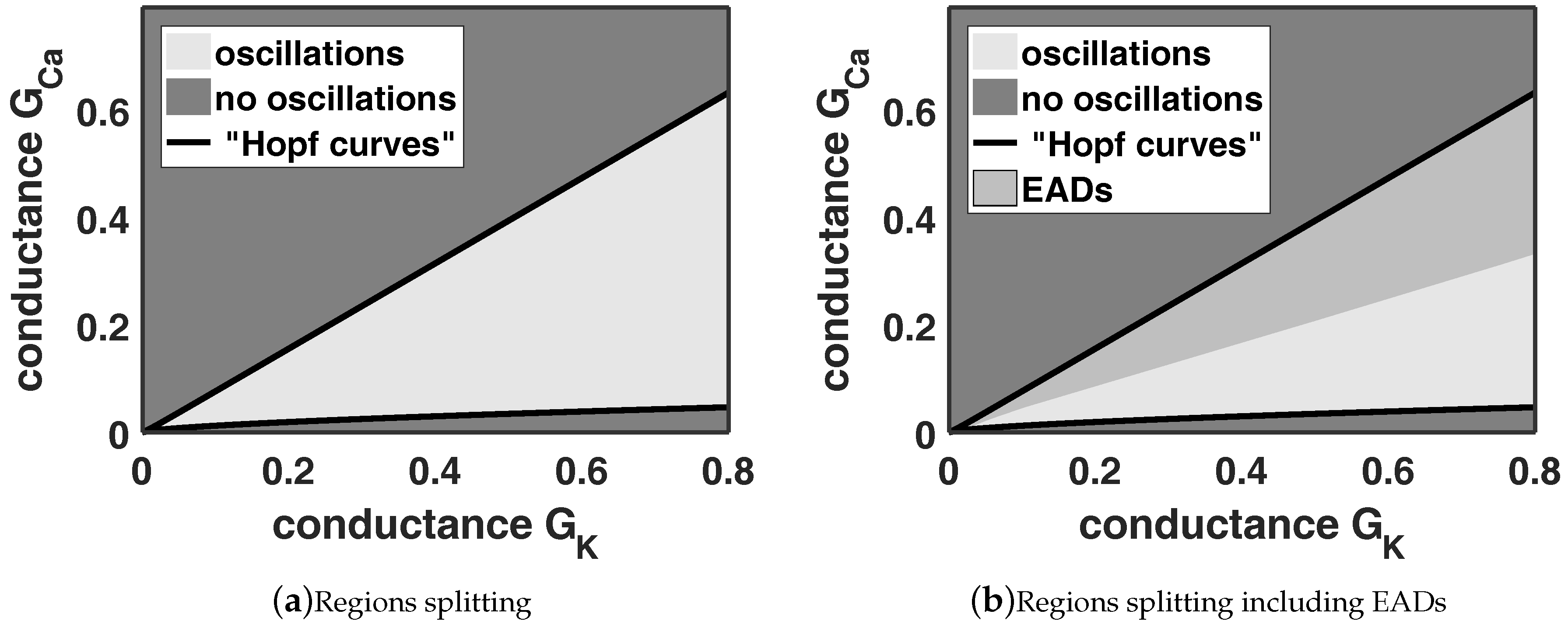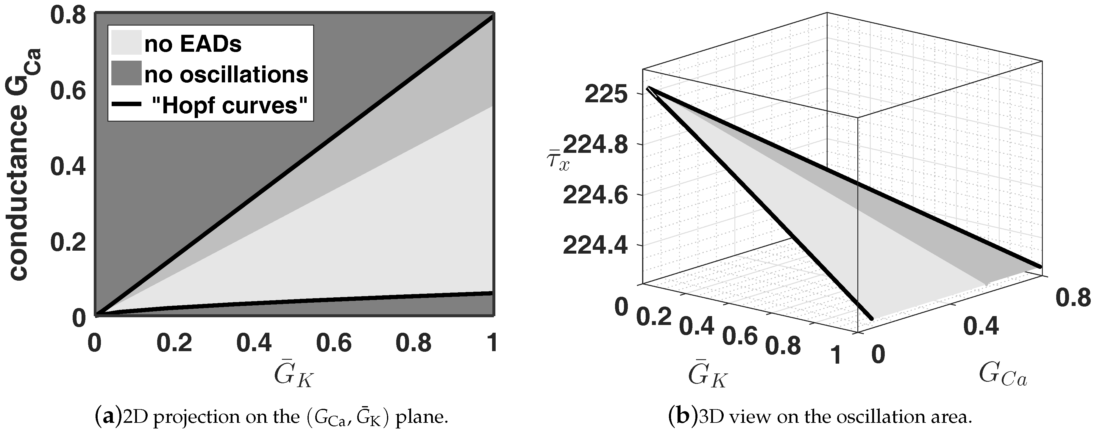Thus, the conditions $a_1>0$, ${\Delta }_2=0$ and $a_3>0$ with condition (3), $f=f_{\infty }$ and $x=x_{\infty }$ yields (numerically) in dependence on $G_{\mathrm{K}}$ and $G_{\mathrm{Ca}}$ the “Hopf-curves” in Figure 7 or Figure 9, respectively. Mainly, we are interested in the separatrix between EADs and no EADs.

In Figure 9 we see that also the region, where EADs appear, is linearly depending on $G_{\mathrm{Ca}}$ and $G_{\mathrm{K}}$. Moreover, the dangerous region is also growing if we increase the two conductances $G_{\mathrm{Ca}}$ and $G_{\mathrm{K}}$. Nevertheless, this investigation shows that one can balance EADs utilising the ion current interaction.

5. Controlling the Early Afterdepolarisations

Our final aim is to control the EADs. To this goal we use our observations from above and the knowledge of the ion current interaction. From Figure 9 we know how we have to shift $G_{\mathrm{K}}$ to smooth out the impact of the enhanced calcium current. However, there are several possibilities to achieve this. First, we can control the EADs by varying the conductance $G_{\mathrm{K}}$ in the potassium current $I_{\mathrm{K}}$ (in the case that the choice of $G_{\mathrm{Ca}}$ yields an EAD) or we can introduce a control parameter $p_{\mathrm{control}}$ and replace $G_{\mathrm{K}}$ by

$$\begin{array}{c}\hfill {\overline{G}}_{\mathrm{K}}:=(G_{\mathrm{K}}-p_{\mathrm{control}}).\end{array}$$

(6)

Then, using $p_{\mathrm{control}}$ as control or bifurcation parameter, respectively, we can balance the EAD. A further approach is to replace $G_{\mathrm{Ca}}$ and $G_{\mathrm{K}}$ by

$$\begin{array}{c}\hfill {\overline{G}}_{\mathrm{Ca}}:=(G_{\mathrm{Ca}}+p_{\mathrm{control}})\mathrm{and}{\overline{G}}_{\mathrm{K}}:=(G_{\mathrm{K}}-p_{\mathrm{control}}),\end{array}$$

(7)

respectively. In this case we control simultaneous both ion currents $I_{\mathrm{Ca}}$ and $I_{\mathrm{K}}$, i.e., we exploit the ion current interaction. Here, we are now able to study the two bifurcation parameter problem from above, but in this bifurcation problem we only vary one bifurcation parameter, i.e., the control parameter. Moreover, we want to emphasise that we shift $G_{\mathrm{Ca}}$ and $G_{\mathrm{K}}$ simultaneous. This yields the same, which we showed exemplary in Figure 6 and corresponds to the regions in Figure 9. Furthermore, we have to highlight that we have to choose the sign of $p_{\mathrm{control}}$ opposed in ${\overline{G}}_{\mathrm{Ca}}$ and ${\overline{G}}_{\mathrm{K}}$, since we know that decreasing of $I_{\mathrm{K}}$ and increasing of $I_{\mathrm{Ca}}$ may yield in both cases EADs. This means that these ion currents behave in same sense reverse (outward and inward currents) and this we want to exploit. The advantage in this approach is also that we do not have to change one current “dramatically”. Please notice in both cases using (6) or (7) we get different values of $p_{\mathrm{control}}$. However, utilising the definitions of ${\overline{G}}_{\mathrm{K}}$ (and ${\overline{G}}_{\mathrm{Ca}}$) in (6) or (7) and relabelling ${\overline{G}}_{\mathrm{K}}$ (and ${\overline{G}}_{\mathrm{Ca}}$) by $G_{\mathrm{K}}$ (and $G_{\mathrm{Ca}}$) we get the conclusion of Figure 9. Finally, we are utilising a further approach, i.e., we consider the following system

$$\begin{array}{c}\hfill \left\{\begin{array}{cc}{\displaystyle \frac{\mathrm{d}V}{\mathrm{d}t}}\hfill & {\displaystyle =-\frac{{\overline{I}}_{\mathrm{K}}+I_{\mathrm{Ca}}}{C_m}=:F_1(V,f,x),}\hfill \\ {\displaystyle \frac{\mathrm{d}f}{\mathrm{d}t}}\hfill & {\displaystyle =\frac{f_{\infty }\left(V\right)-f}{{\tau }_f}=:F_2(V,f,x),}\hfill \\ {\displaystyle \frac{\mathrm{d}x}{\mathrm{d}t}}\hfill & {\displaystyle =\frac{x_{\infty }\left(V\right)-x}{{\overline{\tau }}_x}=:F_3(V,f,x),}\hfill \end{array}\right.\end{array}$$

(8)

with

$$\begin{array}{c}\hfill {\overline{I}}_{\mathrm{K}}:={\overline{G}}_{\mathrm{K}}·x·(V-E_{\mathrm{K}}),{\overline{G}}_{\mathrm{K}}:=(G_{\mathrm{K}}-p_{\mathrm{control}}),{\overline{\tau }}_x:=0.75·({\tau }_x+p_{\mathrm{control}}).\end{array}$$

Here, we again consider only the potassium current to control the effect of the enhanced calcium current. However, we are not only focused on the conductance $G_{\mathrm{K}}$, we are paying attention also to the relaxation time constant ${\tau }_x$. This has influence on the gating variable x and therefore, again on the potassium current, i.e., decreasing of $p_{\mathrm{control}}$ increases ${\overline{G}}_{\mathrm{K}}$ and x. The choices of the signs of the control parameter in ${\overline{G}}_{\mathrm{K}}$ and ${\overline{\tau }}_x$ is again related to the aim to increase the potassium current. This yields the regions in Figure 10.

Here, we see that choosing the approach from (8) yields different region, where oscillations appear, i.e., EADs and no EADs, please cf. Figure 9. We see that – regarding Figure 10a—we have a much bigger range with respect to the conductances $G_{\mathrm{Ca}}$ and ${\overline{G}}_{\mathrm{K}}$, where no EADs appear. To achieve this a reduction of the time relaxation constant ${\tau }_x$ or ${\overline{\tau }}_x$, respectively, is necessary, cf. Figure 10b. Moreover, as a general remark we want to emphasise that all these approaches can be modified, i.e., we can add weight to the control parameter depending on the system specific properties, as we already did in system (8). In system (8), e.g., we can modify ${\overline{G}}_{\mathrm{K}}$ and ${\overline{\tau }}_x$ as follows

$$\begin{array}{c}\hfill {\overline{G}}_{\mathrm{K}}:=(G_{\mathrm{K}}-a·p_{\mathrm{control}})\mathrm{and}{\overline{\tau }}_x:=b·({\tau }_x+c·p_{\mathrm{control}}),\end{array}$$

(9)

where $a,c\in {\mathbb{R}}^{+}$, $a\ne c$ and $0<b$ or similar modifications. Especially, in this paper we are focused on balancing the enhanced calcium current via the increasing the potassium current. Please remark also that all these approaches we have for $p_{\mathrm{control}}=0$ and $b=1$ the initial situation. Moreover, we know that we can compensate the enhancement of the calcium current by increasing the potassium current.

Furthermore, notice that to balance an EAD induced by an enhanced calcium current the control parameter $p_{\mathrm{control}}$ in system (8) has to be negative. Using the approach (8) together with (9) and the choices $a=b=c=1$ yields also a different regions as in Figure 9, but the ”Hopf-curves” are still less steep as in Figure 10. This means we can control the slope of the “Hopf-curves”.

Finally, we want to remark that this approach we can also use for more general systems, e.g., including the sodium current $I_{Na}$ or relaxation time constants, which are depending on the voltage V, cf. [17]. This yields then more possible choices of the parameters and the parameter space will grow, but this has also potential to study and to control cardiac arrhythmia in a more specific way.

6. Discussion

In this paper, we studied the Hodgkin-Huxley model from [1] to investigate the occurrence of EADs related to an enhanced calcium current and the ion current interaction of the potassium and calcium current. For this aim we used the bifurcation theory and the numerical bifurcation analysis to derive a separatix between EADs, i.e., mixed mode oscillations [30,31] with one large and one or more small oscillations, and no EADs in system (1), cf. Figure 9. It turns out that our system loses stability and oscillates (in the sense of periodic orbits mentioned in Section 3) between two Andronov-Hopf bifurcations, where EADs as well as no EADs appear (periodic orbits). In this region stable periodic orbits occur, where the number of small oscillations are depending on the numbers of (unstable) limit cycle branches, cf. Figure 4 and [28], where we adumbrated this fact.

Moreover, we showed that no EADs occur in a region between the supercritical Andronov-Hopf bifurcation (related to small values of the conductance $G_{\mathrm{Ca}}$) and the first LP of cycles of the first Hopf continuation—which generically corresponds to a turning point of a curve of limit cycles—from this supercritical Andronov-Hopf bifurcation, cf. Figure 4. This corresponds also with the circumstance that EADs may appear by the enhancement in the calcium current. Please notice that also the phenomena of isolas may occur for different settings of the system parameters, cf. for instance [28], but not in our setting, please cf. Figure 5. Furthermore, we restricted our bifurcation diagram to the first two limit cycle branches. The continuation from an Andronov-Hopf bifurcation is comparably easy and fast, while already the continuation of the second limit cycle branch becomes challenging and needs a lot of computational power. Since we are interested in the region, where EADs appear, and because of these numerical efforts, it makes sense to focus on the first limit cycle branch (mainly if one consider a multiple bifurcation problem).

Furthermore, we highlighted that the effect of an enhanced calcium current can be compensated by an increasing of the potassium current, cf. Figure 6. Since we considered only the toy model (1) depending on two ion currents our study is limited to the ion current interaction of the potassium and the calcium current. However, a similar result, we can expect also from the interaction of the potassium and sodium current. Then, these observations motivate the study of system (1) as a multiple bifurcation problem, i.e., our investigation was not only focused on one bifurcation parameter. Please note that EADs can be induced by an increase of the L-type calcium conductance and by the application of potassium current blockers, cf. [3]. Using two bifurcation parameters, yields that the area, where oscillations in system (1) appear, increases by increasing of $G_{\mathrm{Ca}}$ and $G_{\mathrm{K}}$ (simultaneously), see Figure 9.

At this stage we want to emphasise, that the study of model (1) as a multiple bifurcation problem with up to five (most important) parameters yields further cognitions, cf. Figure 8 and Figure 9. Moreover, we can use this approach to study more general Hodgkin-Huxley models or we can utilise this strategy to show that EADs related to a reduction of the potassium current can be compensated by a decreasing of the calcium current.

Summarising, we have shown four main result. Obviously, the increasing of the calcium current may yield EADs. Second, one can use an increased potassium current (e.g., induced by some drug) to compensate EADs derived by an enhanced calcium current (e.g., induced by ion channel disease). On the other hand, one can also balance EADs induced by a reduced potassium current, via the reduction of the calcium current. This means if one is not able to decline the influence of a potassium blocker, one may vanish the effect of the potassium blocker by a “calcium blocker”. Third, from our study one can expect that EADs may occur via a combination of an enhanced calcium current and a reduced potassium current, cf. [3]. Therefore, the effect of both phenomena can be mutually reinforcing. Thus, EADs may also appear in a “safe region” focused only on one ion current. Fourth, we showed that EADs related to an enhancement in the calcium current are not Hopf-induced in the sense of the geometric singular perturbation theory [32].

Furthermore, in the paper we used several control approach to balance the effect of the enhancement in the calcium current. Here, it turns out that EADs can be compensated using the approach in (8) in a very effective way. The reason is that we increase simultaneous $G_{\mathrm{K}}$ and ${\tau }_x$, where we added a weight to ${\tau }_x$, i.e., we increased the speed of the gating variable x. This yields very different regions if we compare Figure 9b and Figure 10a.

In addition, if we study models containing also a sodium current, then the effects of the different ion currents can be balanced by increasing or decreasing the other ion currents. The investigation of the three main ion currents by considering three parameters $G_{\mathrm{Ca}}$, $G_{\mathrm{K}}$ and $G_{\mathrm{Na}}$ will yield a three dimensional parameter space and therefore, we will have more possible choices to prevent the EADs. Even more, we are able to investigate and to understand the ion current interactions by means of the bifurcation theory in a very general way, which is useful for the treatment of cardiac diseases. This short study emphasise the importance of the inclusion of the two or three main ion currents, which are related to the occurrence of EADs and the beneficing of bifurcation analysis in the investigation of cardiac arrhythmia.

Finally, we want to outline that our study was only focused on a toy model of dimension three containing two ion currents and it is as a future project mandatory to consider more complex models to be able to understand all effects yielding EADs. Nevertheless, we can use our approach also in more complex situations for the investigation of EADs. Beside the extension of this study to more general ion current models, one has to think about to the study of multi-domain models to be able to study the effect of EADs on the complete heart. A first good starting point would be to observe a mono-domain model as in [4].