The Impact of Global Sensitivities and Design Measures in Model-Based Optimal Experimental Design
by
 ,
,
René Schenkendorf
1,2,*,† ,
,
Xiangzhong Xie
1,2,3, 
Moritz Rehbein
2,4,
Stephan Scholl
2,4 and
Ulrike Krewer
1,2 1
Institute of Energy and Process Systems Engineering, TU Braunschweig, Franz-Liszt-Straße 35, 38106 Braunschweig, Germany
2
Center of Pharmaceutical Engineering (PVZ), TU Braunschweig, Franz-Liszt-Straße 35a, 38106 Braunschweig, Germany
3
International Max Planck Research School (IMPRS) for Advanced Methods in Process and Systems Engineering, Sandtorstraße 1, 39106 Magdeburg, Germany
4
Institute for Chemical and Thermal Process Engineering, TU Braunschweig, Langer Kamp 7, 38106 Braunschweig, Germany
*
Author to whom correspondence should be addressed.
†
Current address: Institute of Energy and Process Systems Engineering, TU Braunschweig, Franz-Liszt-Straße 35, 38106 Braunschweig, Germany.
Processes 2018, 6(4), 27; https://doi.org/10.3390/pr6040027
Submission received: 14 February 2018
/
Revised: 15 March 2018
/
Accepted: 19 March 2018
/
Published: 21 March 2018
(This article belongs to the Special Issue Feature Papers for the Fifth Year Anniversary of the Founding of Processes)
Abstract
:In the field of chemical engineering, mathematical models have been proven to be an indispensable tool for process analysis, process design, and condition monitoring. To gain the most benefit from model-based approaches, the implemented mathematical models have to be based on sound principles, and they need to be calibrated to the process under study with suitable model parameter estimates. Often, the model parameters identified by experimental data, however, pose severe uncertainties leading to incorrect or biased inferences. This applies in particular in the field of pharmaceutical manufacturing, where usually the measurement data are limited in quantity and quality when analyzing novel active pharmaceutical ingredients. Optimally designed experiments, in turn, aim to increase the quality of the gathered data in the most efficient way. Any improvement in data quality results in more precise parameter estimates and more reliable model candidates. The applied methods for parameter sensitivity analyses and design criteria are crucial for the effectiveness of the optimal experimental design. In this work, different design measures based on global parameter sensitivities are critically compared with state-of-the-art concepts that follow simplifying linearization principles. The efficient implementation of the proposed sensitivity measures is explicitly addressed to be applicable to complex chemical engineering problems of practical relevance. As a case study, the homogeneous synthesis of 3,4-dihydro-1H-1-benzazepine-2,5-dione, a scaffold for the preparation of various protein kinase inhibitors, is analyzed followed by a more complex model of biochemical reactions. In both studies, the model-based optimal experimental design benefits from global parameter sensitivities combined with proper design measures.
1. Introduction
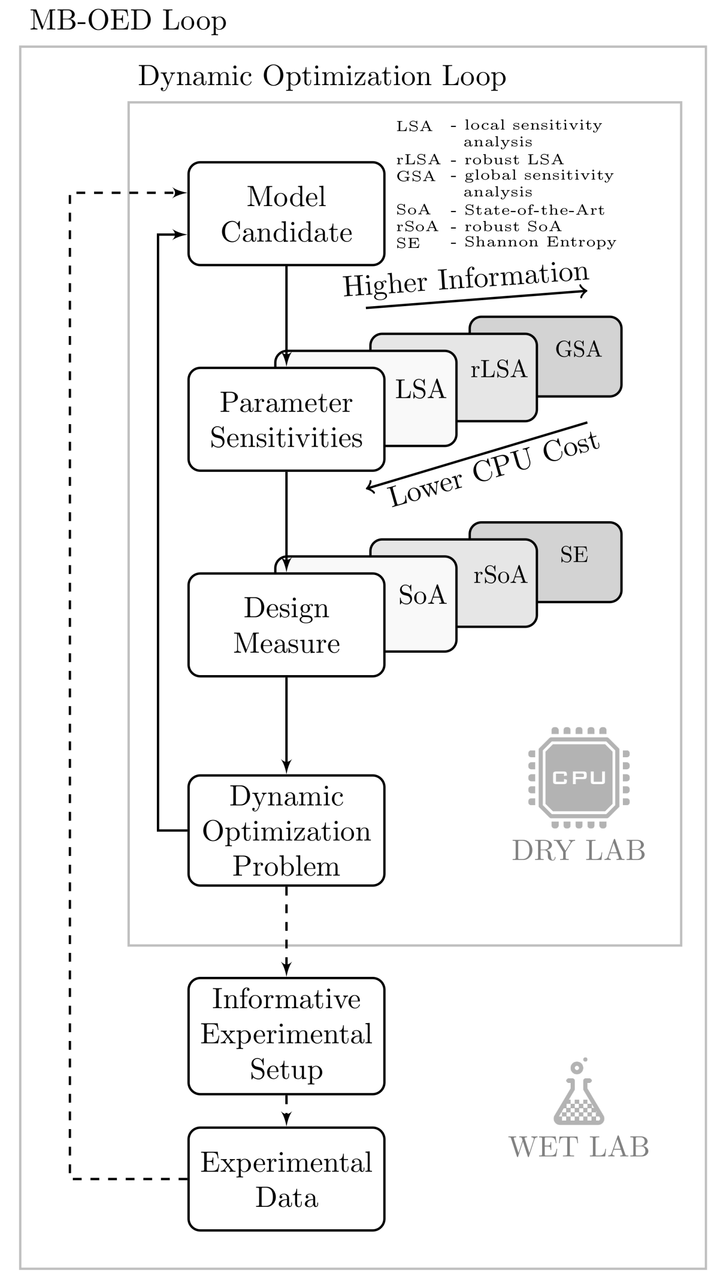
Mathematical models have been proven to be an indispensable tool in chemical engineering research and design. For instance, model-based and computer-aided concepts are the standard in process analysis [1,2,3], process design [4,5,6], and condition monitoring [7,8,9]. To gain the most benefit of model-based approaches, the model-building process itself becomes a crucial step in computer-aided process analysis and design. When it comes to mathematical modeling and model-based design, model developers are challenged by the problem of providing meaningful results. The situation is the same for the computer-aided process design of pharmaceutical processes and active pharmaceutical ingredients (API) syntheses [10,11]. In addition to a proper model structure determining the interconnection of involved quantities and species, the most critical part is to identify related model parameters [12,13]. When assuming a correct model structure, any mismatch of measurement data and simulation results is mainly attributed to biased model parameters. Optimal tuning of those model parameters according to the experimental data is an essential step in the process of model development where model parameters are iteratively adapted until simulation results fit the given measurement data best [12,14]. Thus, the quality of model-based results depends significantly on the quality of the parameter estimates. The parameter quality itself, however, depends on the quality of the measurement data and the conducted experiments, respectively. The operating conditions of the experiment indirectly determine the sensitivity of the model parameters to the simulation results. The parameters with a high sensitivity are likely to be reliably identified. Model parameters with low sensitivity, in turn, can be changed by an order of magnitude with little to no effect. Any attempt at a manual or algorithmic tuning of such insensitive parameters is error prone by definition. To avoid this kind of ill-posed parameter identification problem, model-based optimal experimental design (MB-OED) comes into play [14,15,16,17]. The aim of MB-OED is to redesign the experimental setup ensuring high sensitivities of all parameters over the course of the experimental run. To this end, a dynamic optimization problem has to be solved, which typically includes the following generic steps; see also Figure 1 for their interaction. First, the parameter sensitivities of a given model candidate have to be quantified. Based on the parameter sensitivities, a suitable design measure is defined and evaluated, which translates parameter sensitivities into algorithmically evaluable quantities. After specifying potential design variables of the experimental setup, which are practically feasible and allow the control of the main process states, an optimizer routine adapts the experimental setup iteratively. The resulting optimal design variables determine the setup of the next experimental run, which is expected to produce new informative measurement data. These data, in turn, represent operating conditions at which, in general, the model parameters show an increased sensitivity leading to more precise parameter estimates. This MB-OED loop is reiterated until the parameter estimates fulfill the needs of particular modeling tasks. While following the proposed work flow, i.e., (1) sensitivity quantification, (2) design measure evaluation, (3) dynamic optimization, and (4) running an optimally designed experiment, the final result depends critically on the sensitivity measure and its proper implementation. Any improper choice at this point will lead to sub-optimal experimental designs and non-informative data. Thus, reliable sensitivity measures are mandatory for MB-OED to provide the most informative data possible. This aspect is particularly relevant for syntheses of active pharmaceutical ingredients, where typically the number of novel drugs and the number of experimental runs are limited.
In the literature, most implementations of MB-OED are based on local sensitivities as part of the Fisher information matrix (FIM) [12,14,16,18,19,20]. Technically, the inverse of the FIM is used to approximate the covariance matrix of the parameter estimates [12,14,18]. This local approach assumes a linear relation between parameter perturbations and model responses—at least locally in the neighborhood of the correct reference parameter values. As the actual parameter values, however, are typically unknown, their current best estimates have to be inserted instead. Thus, the calculated local sensitivities may fall short as they do not describe the underlying nonlinearities and because of biased reference parameters [16,21]. To compensate for biased references, sensitivity gradients can be evaluated at various but representative parameter values within the given parameter domain following a Bayesian experimental design principle [22,23,24]. Here, the basic idea is to get an improved approximation of the local sensitivities based on an averaged measure [25]. Nonlinear effects, however, still remain unaddressed. Most parameter identification problems of practical relevance in the field of pharmaceutical processes are characterized by nonlinear impacts of model parameters on model responses [19]. Thus, local sensitivities, in general, might lead to oversimplified inferences, less robust experimental designs, and an unnecessarily high number of experimental reiterations [21]. This last point, as mentioned previously, is of critical relevance when analyzing novel but exceedingly rare drug candidates.
Alternatively, in the last decade, the implementation of global sensitivities for MB-OED has been introduced in the literature [25,26,27]. Global sensitivities by definition take into account nonlinear effects and multivariate parameter dependencies. To the best of the authors’ knowledge, the usefulness of GSA and its practical implementation for pharmaceutical and (bio)chemical processes have not been analyzed thus far. This manuscript shows how global sensitivities can be determined efficiently by a deterministic sampling rule even for complex models with a large number of model parameters, which makes GSA available for advanced MD-OED strategies.
The focus of this study is to compare and assess different parameter sensitivity measures, as well as an analysis of the need for novel design criteria for MB-OED. In particular, local sensitivity analysis (LSA), robust local sensitivity analysis (rLSA), and global sensitivity analysis (GSA) are introduced. In addition to state-of-the-art (SoA) design criteria, further alternatives are discussed in the following. Thus, the paper unfolds as follows. First, the basics of parameter sensitivity analysis as a key element of optimal experimental design are presented in Section 2. Here, the focus is also on the efficient implementation of global parameter sensitivities. Based on the derived sensitivity measures, optimal design metrics are derived in Section 3. In Section 4, the proposed concept is illustrated by two pharmaceutically relevant processes, the homogeneous synthesis of 3,4-dihydro-1H-1-benzazepine-2,5-dione, a scaffold for the preparation of various protein kinase inhibitors, and a more complex biochemical synthesis example. The conclusions are given in Section 5.
2. Sensitivity Measures
In the literature, different methods and concepts for parameter sensitivity analysis (SA) exist, ranging from local to global approaches [28,29,30]. In the context of MD-OED, sensitivity analysis is an inherent part of the optimization problem aiming to provide an optimal range of sensitivities over the course of the experimental run. In the following, we consider nonlinear state-space models of the form
where is the vector of model states (), is the vector of system inputs (), is the vector of parameters (), and is the vector of model outputs (). Typically, only a minor subset of the states can be measured directly or indirectly; i.e., . The proposed concepts can be extended to more general model types, e.g., differential algebraic or partial differential equation systems, but are discussed here solely for nonlinear state space models for the sake of clarity. As the model parameters are typically unknown, they have to be identified by minimizing the error between simulation results, , and measurement data, . By following a maximum likelihood estimation procedure and assuming additive white measurement noise with a standard deviation of one [14], the parameter identification problem simplifies toRegarding the least squares problem, the parameter identification problem reads as
where K is the number of measurement time points. According to the measurement noise and the Doob–Dynkin lemma [31], the identified model parameters are random variables as well; for example, measurement uncertainties induce stochastic parameter uncertainties. The resulting parameter uncertainties, in turn, are determined by the data quality and parameter sensitivities alike.
2.1. Local Parameter Sensitivities
In practice, local sensitivities are the standard for analyzing the effect of parameter variations on model-based results [28,29,32]. Local sensitivities are typically expressed by partial derivatives of the j-th model output, , with respect to the i-th model parameters, , as
and summarized by the sensitivity matrix while and . In the field of dynamical systems, the governing equations of the original model (Equation (2)) have to be extended by sensitivity terms of the states, , which are solved in parallel according to
Thus, the output sensitivities can be expressed as
Alternatively, the gradients (Equation (4)) can be calculated with various numerical methods, e.g., automatic differentiation or finite differences. Here, the interested reader is referred to [32,33] and references therein.
Technically, local sensitivities provide information about the relevance of model parameters in the neighborhood of a reference point within the defined parameter space, a reference which is typically unknown for most practical problems. In an ideal world, hypothetically, the reference point corresponds to the exact model parameters. Moreover, the general idea of local SA measures is based on linearization principles; i.e., the original, nonlinear model (Equation (2)) is linearized at the (unknown) reference point. Thus, nonlinear effects are ignored although the analyzed models may have strong nonlinearities involved [21]. The resulting approximation errors may render the outcome of such a sensitivity analysis meaningless and difficult to interpret in general. To compensate for the dependency of unknown reference points, a multi-point averaging approach can be applied as described in the following sections.
2.2. Robustification: Multi-Point Averaging Approach
As the reference points for the sensitivity gradients are typically unknown, local sensitivities may provide artifacts; i.e., insensitive parameters are identified as sensitive or vice versa. To avoid this kind of mis-classification, an averaged version of the sensitivity matrix (Equation (4)) seems to be a more robust measure [25,34] following a Bayesian experimental design principle [22,23,24] and is defined as
where is the expected value, is the support domain, and the probability density function (PDF), , represents the assumed parameter variation of the i-th parameter. According to Equation (7), for linear problems, the proposed concept simplifies to the local SA expression [25]. In most practical scenarios, there exists no analytical solution of Equation (7). Thus, Monte Carlo (MC) simulations are evaluated instead to solve a discretized approximation resulting in a multi-point averaging approach equal to
where represents the k-th realization of the i-th parameter according to the given PDF. The sample number, N, determines the total number of function calls of Equation (5) needed to approximate the averaged sensitivity measure, i.e., for each parameter realization, , Equation (5) has to be vectorized and solved in parallel with the dynamic model (Equation (1)) that is also evaluated for . By using instead of the standard local quantities , the resulting parameter sensitivities are more representative of nonlinear problems [34,35,36] and may provide a reliable base for subsequent MB-OED studies. As standard MC simulations might become prohibitive in terms of computational load, efficient sample-based approaches are mandatory and will be discussed in more detail in Section 2.4.
The multivariate interaction, however, of the analyzed model parameters is still not taken into account appropriately by the multi-point averaging concept. Here, the framework of global sensitivities seems to be more suitable to rank vaguely known parameters and to quantify their interactions.
2.3. Global Parameter Sensitivities
Global sensitivity measures treat parameters, , and model outcomes, , as random variables and aim to quantify the amount of variance that each parameter, , adds to the total variance of the output, [29,37,38]. In detail, the parameter ranking is done by the amount of output variance that disappears when the i-th parameter is assumed to be known, . For this particular parameter, a conditional variance, , can be derived. Here, the subscript indicates that the variance is taken over all parameters other than . As , in reality, is a random variable, the expected value of the resulting conditional variance, , has to be analyzed. The subscript notation of indicates that the expected value is taken only over the parameter itself. Finally, the total output variance, , can be split into two additive terms [29] equal to
Here, the variance of the conditional expectation, , represents the contribution of parameter to the total variance . The normalized expression given in Equation (10) is known as the first-order Sobol sensitivity index [29] and is used in the following to analyze parameter sensitivities and multivariate parameter interactions, respectively:
Similar to the multi-point averaging approach (Section 2.2), the integral terms associated with , , and are commonly evaluated with MC simulations [39]. For global sensitivity studies of complex models, MC simulations have prohibitive computational costs. Thus, while implementing an MB-OED strategy based on global sensitivities, highly efficient methods have to be used. The most relevant concepts in this direction are outlined in the next section.
2.4. Implementation Aspects
Over the last two decades, various methods have been developed to calculate Sobol indices efficiently. The most frequently used approaches are based on advanced MC simulations and polynomial chaos expansion (PCE) principles [40]. In comparison to ordinary MC simulations, advanced sampling concepts aim for a better convergence rate by an improved space-filling sampling strategy, i.e., to avoid clustering effects, as well as gaps in the p-dimensional sampling space [41]. Please note that p represents the dimension of the random vector, i.e., the number of not perfectly known model parameters. For instance, so-called quasi-MC methods have a convergence rate of , which for low-dimensional problems can lead to a significant reduction in computational costs in comparison to for ordinary MC [41]. On the other side, PCE-based approaches aim to replace the original CPU-intensive model with a handy and easy-to-evaluate surrogate model first. Then, some characteristics of the derived PCE models are used to express global sensitivities analytically by using the PCE coefficients directly or to run additional MC simulations at low computational costs [42]. The parameterization of the PCE model, however, requires a significant number of reference simulations of the original model. Both concepts, advanced MC methods and PCE, might be prohibitive for MB-OED problems because of their computational costs. Highly efficient uncertainty handling methods are needed instead. Here, the point estimate method (PEM) provides a fair compromise in terms of CPU load and accuracy [43,44].
The fundamental idea of the PEM is to choose sample points, , and associated weights, , in accordance with the first central moments of given random variables [43]. However, in comparison to MC simulations, these sample points are generated deterministically and not randomly. Assuming a three-dimensional parameter problem, for instance, the resulting sample set reads as
The generator function, , creates the sample set by permuting an element of the original random vector one by one by the amount of . Thus, the scaling parameter, , controls the spread of the sample points in the p-dimensional parameter space. To calculate the expected value, the discretized integration problem reads as
with and assuming a standard Gaussian distribution. Moreover, the overall precision of the PEM can be increased gradually by considering higher-order central moments of . The more precise approximation scheme [44,45] results in
where implies the simultaneous variation of two elements of the given parameter vector . Thus, the number of generated sample points, , scales quadratically with for a p-dimensional parameter problem: a good balance of computational load and approximation power.
The four unknown coefficients, , , , and , can be expressed analytically as
where is the zeroth central moment, the second central moment, the fourth central moment, and a bivariate central moment. Depending on the PDFs and their central moments, different PEM coefficients are derived. For instance, specifications of different PDFs and their corresponding PEM coefficients are given in Table 1 and Table 2, respectively. Here, three different PDF types are considered: (i) normal distribution to represent the uncertainty range of well-known parameter variations; (ii) uniform distribution for cases where almost no information about the parameter variation is available; and (iii) triangle distribution to represent expert knowledge of parameter variations; i.e., the most likely parameter values and plausible upper and lower bounds. Within the individual distribution classes, any desired realization can be derived with a linear transformation step without loss of approximation accuracy, while non-symmetric or non-parametric distributions can be represented by iso-probabilistic but nonlinear transformation rules [42], which might introduce additional approximation errors.
Once the deterministic sample points have been derived, the mean and the variance of the model simulations can be approximated as
Obviously, Equation (18) can directly be applied to approximate the averaged local sensitivity measure (Equation (7)), whereas the denominator of the Sobol indices (Equation (10)) is approximated with Equation (19). The calculation of the conditional variance terms of the numerator in Equation (10) is given in the following.
The overall set of generated sample points of the PEM provides nested subsets of sample points representing the conditional variance terms. According to the numerator of Equation (10), the expected value is taken over all but the i-th parameter; i.e., the -value of parameter i is set to zero. The variance, however, is taken exclusively for the i-th parameter; i.e., the corresponding entry is reset to its original distribution-dependent value. Only the weights, and , have to be adapted to a one-dimensional problem while leaving the overall PEM samples unchanged, i.e., there is no need for additional costly simulation runs. Please note the weight is set equal to zero; i.e., sample points generated via are not considered at this point. The described procedure is illustrated in Figure 2 assuming a three-dimensional parameter problem. In Figure 2a, the original sample set generated via Equation (11) is shown. Next, in Figure 2b, three different expected values are determined for via the three differently colored sample subsets and different values, respectively. When using these three derived expected values for , the conditional variance of can be approximated (Equation (10)). The same procedure is repeated for parameter (Figure 2c) and parameter (Figure 2d) to derive the desired Sobol indices. Please note that the derived samples are not used to quantify the information content [16,46,47], but to quantify the uncertainty of the local sensitivities or to directly derive global parameter sensitivities. In [48,49], the performance of the PEM for calculating global parameter sensitivities and uncertainty analysis is discussed in more detail. Here, the PEM provides appropriate approximations at low computational costs compared to Monte Carlo simulations. In the next step, from these sensitivity measures, the most MB-OED-relevant features have to be extracted by defining proper optimal design measures.
3. Optimal Design Measures
The actual optimization step of the MB-OED framework calls for a decision criterion that has to express the quality of the analyzed experimental configuration regarding parameter sensitivities. To this end, typically, representative scalar values are chosen for and evaluated with an optimization routine. In the literature, well-known criteria for local sensitivities exist and are summarized below followed by more general global design criteria.
3.1. Local Design Measures
The starting point for most local design criteria is an approximation of the parameter (co)variance matrix, which is defined as
Based on the Cramér–Rao inequality [14] and local sensitivities (Equation (4)), the lower bound of the parameter (co)variance matrix assuming an unbiased estimator reads as
where the FIM is given by
represents the (co)variance matrix of the measurement data, which simplifies to a diagonal matrix assuming uncorrelated data samples. To formulate an optimization problem, a scalar function of the derived parameter (co)variance matrix is typically evaluated and minimized. Note that the inverse FIM is used as an approximation of the parameter covariance matrix in what follows, . A common class of these indicators is the so-called alphabetic family of design criteria [14,18] as given in Table 3. Here, and are the maximum and minimum eigenvalues of , respectively.
Which of these criteria leads to the best optimal experimental design is difficult to predict and depends on the analyzed problem at hand. Moreover, in many practical situations, the involved model parameters are highly correlated; for example, credible parameter estimates are challenging and sometimes impossible to derive for individual parameters. For that reason, dedicated anti-correlation criteria were proposed, aiming to reduce the parameter correlation while increasing the information content of the measurement data at the same time [50]. Here, linear parameter correlation is expressed as
with . The dominating correlation coefficients are selected directly or added as constraints to parameter variance measures [50], respectively. The basic notation reads as
where and with are the two most dominant correlation coefficients. As the (co)variance matrix is derived by the FIM (Equation (21)), these anti-correlation criteria depend on local parameter sensitivities (Equation (4)), too. As discussed in Section 2.1, local sensitivities may lead to crude approximation errors and sub-optimal experimental designs. In principle, the approximation error can be reduced by the multi-point averaging concept as proposed in Section 2.2 but still ignores nonlinear and multivariate effects as explained below.
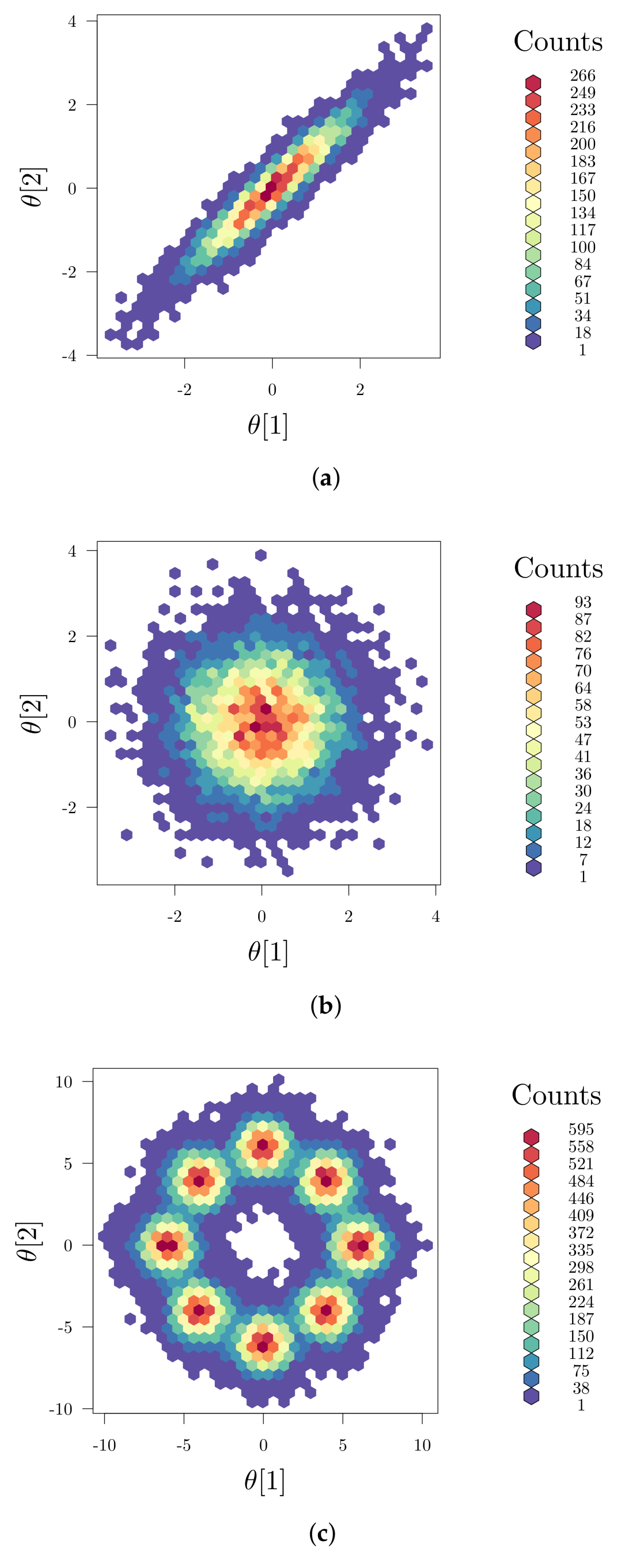
While the anti-correlation strategy was successfully demonstrated for chemical and biochemical processes [50,51], it addresses linear parameter correlation solely, which, however, does not imply parameter independence [52]. Thus, nonlinear parameter correlations are neglected, but might be of relevance in MB-OED as well. In Figure 3, parameter dependencies are illustrated showing linear correlation (Figure 3a) and no correlation (Figure 3b) of two model parameters. In Figure 3c, however, the linear correlation coefficient (Equation (23)) is zero, but nonlinear interaction patterns are clearly visible. Ideally, the parameter estimate of one parameter should not impact the estimation outcome of other parameters. The same holds true for multivariate parameter interactions, i.e., the joint effect of more than two parameters that are also not considered by the linear anti-correlation measure introduced in Equation (24). To address nonlinear parameter correlations and multivariate parameter interactions properly, global sensitivities and corresponding optimal design measures have to be analyzed instead.
3.2. Global Design Measures
The additional insight given by global sensitivity measures (see Section 2.3) provides a new perspective on MB-OED [19,25,26,53]. As shown in Table 4, local design criteria (Table 3) are typically generalized to hold also for global sensitivities by substituting local sensitivities (Equation (4)) via global sensitivities (Equation (10)) [26,53].
Thus, parameter uncertainties are taken into account naturally. Suboptimal results in MD-OED caused by misspecified reference points for local sensitivities (Equation (4)) can be avoided as much as possible by analyzing the entire PDF of the analyzed model parameters. Moreover, GSA provides additional insight into parameter dependencies, which can be included in the experimental design criteria as well. One attempt in this direction was made recently in [53], where so-called additive sensitivity indices are introduced as modified Sobol indices. Here, the key idea is to account for multivariate parameter interactions and dependencies that impact the overall quality of parameter estimates similar to individual parameter sensitivities. The usage of GSA to express generalized sensitivity matrices for MB-OED may pose some risk as well: (1) Not all GSA-based measures simplify to local measures for linear problems [25], which may lead to sub-optimal experimental designs and counter-intuitive outcomes; (2) including sensitivities of parameter combinations directly in a generalized GSA measure [53] might increase parameter dependencies; i.e., parameter correlations are amplified while limiting individual parameter contributions and, therefore, result in more challenging parameter identification problems; and (3) as the introduced GSA measures are normalized by the total variance factor, the calculated design may lead to an improved parameter sensitivity spectrum, but of lower sensitivities for individual parameters. Thus, the individual Sobol indices are optimized just by decreasing the term of Equation (10), meaning worse estimates for all model parameters.
To avoid the workaround of transferring global sensitivities into the local framework, the Shannon entropy as a general information measure [54] might be a helpful expression to calculate the desired features for global MB-OED. Intuitively, an optimal experimental design should fulfill the following features: (1) first, after running an experiment, the derived data have to ensure a balanced sensitivity of all parameters; i.e., all parameters should be practically identifiable. Thus, the corresponding Shannon entropy of the parameter sensitivities has to be at its maximum and the given criteria at its minimum (Table 5); i.e., there is a uniform distribution of the first-order Sobol indices. Note that refers to the averaged sensitivities covering all sample time points; (2) at a single time point , however, it is desirable that only a very limited number of parameters contribute at the same time, i.e., to minimize (nonlinear) correlation effects. Thus, the Shannon entropy covering global sensitivities at a single time point has to be at its minimum; (3) to address multivariate parameter interactions and to minimize them, the gap between the sum of first-order Sobol indices and its theoretical maximum value of one is evaluated ; see Table 5. Here, a sum of first-order Sobol indices close to one corresponds to low parameter interactions, i.e., a well-posed parameter identification problem; and, (4) finally, the overall output variance has to be incorporated as well: the higher the better. A high output variance (Equation (19)) indicates a high parameter sensitivity, which is a prerequisite for credible parameter estimates. Please note that, for consistency, the related cost functions are given as a minimization problems.
In the next step, MB-OED results based on the proposed global design measures are critically compared with the outcome of the traditional local sensitivity measures. To this end, various experimental design conditions are evaluated for two representative case studies in the field of pharmaceutical manufacturing.
4. Case Studies
4.1. Synthesis of an API–Scaffold (DHBD)
During the early stages of API process development, different properties of the unit operations involved are analyzed in order to characterize and to optimize the synthesis as well as the downstream route. Reaction rates are regarded as key descriptors of the synthesis progression as they depend on, temperature, and time. As a first case study for MB-OED, the homogeneous synthesis of 3,4-dihydro-1H-1-benzazepine-2,5-dione (DHBD) from the enolized 3-oxocarboxylic ester in wet dimethyl sulfoxide (DMSO) under neutral conditions and at elevated temperatures is presented; see Figure 4.
DHBD and its derivatives are pharmaceutically relevant scaffolds utilized for the synthesis of various protein kinase inhibitors and anticancer agents [55,56,57,58,59,60]. In traditional reaction optimization studies, isothermal syntheses at various temperatures are carried out one by one, and the syntheses are analyzed with offline high-performance liquid chromatography (HPLC) in order to determine reaction kinetics. However, HPLC measurements are tedious in sample preparation and need increased amounts of reactant, which might not be available in the very early stage of API development. Alternatively, we implement the fast-sampling and labor free in situ attenuated total reflectance Fourier transform infrared (ATR-FTIR) spectroscopy in order to quantify the reactant concentration and, subsequently, to calculate reaction rate constants without the need for manual sampling. Combined with non-isothermal temperature profiles during the course of the reaction, temperature-dependent kinetic data, e.g., reaction rate constants at different temperatures and therefore Arrhenius parameters and of the reaction under study, can be derived from a single experimental run [61]. The quality of the derived reaction rate constants critically depends on the design of the applied non-isothermal temperature profile.
In what follows, we assume an Arrhenius rate expression:
where k is the rate constant, T is the absolute temperature, R is the ideal gas constant, is the pre-exponential frequency factor, and the activation energy. Because of the inherent correlation of the two Arrhenius parameters, and , the parameterization of the Arrhenius equation (Equation (25)) is challenging. That is, independently of the applied experimental setup the correlation cannot be reduced for the Arrhenius rate [62,63] expression. At best, a parameter transformation might be applied to mitigate the correlation effect but changes the meaning of the identified parameters alike [64]. Thus, for this particular MB-OED problem, any anti-correlation criteria, which include the modified -criterion as well, fail. Only the overall uncertainty of the parameter estimates can be reduced in principle. For this very reason, we first derive MB-OED results based on local sensitivities (Equation (4)) and the classical D-criterion (Section 3), which is expected to minimize the volume of the parameter confidence ellipsoid [14]:
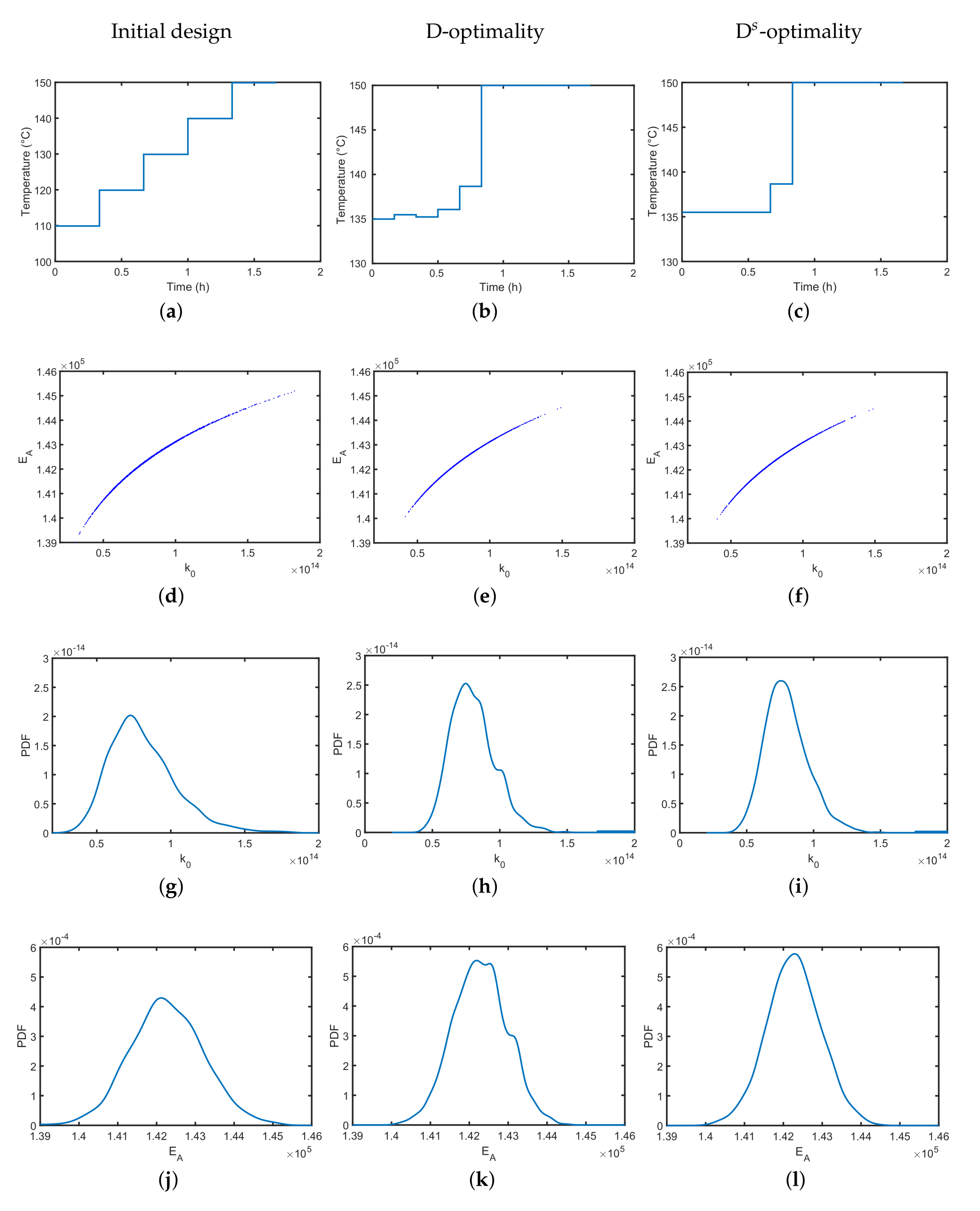
The optimal experimental design problem is described in Equations (26)–(28), where Equation (27) is the dynamic reaction model with the DMSO concentration , and Equation (28) is the temperature constraint. A temperature profile divided into equidistant and constant subintervals is assumed. For all intervals, upper and lower temperature bounds are given as 100 and 150 while assuming continuous measurements of DHBD. Technically, the Matlab® (R2017a) optimizer fmincon is used to derive an optimal temperature profile; i.e., a profile that provides the most informative data and lowest parameter variations. The performance of the original and optimal temperature profile is validated with 2000 Monte Carlo simulations, where for each simulation and parameter identification, respectively, artificial experiment data are assumed with additive white noise. In Figure 5a, we show a reference temperature profile of five temperature steps of equal step-size, which was chosen by educated guessing. The reference profile might already be a good choice to identify the two Arrhenius parameters as it covers the whole temperature range without any obvious preferences. In Figure 5b, we see that the estimates are of finite variation, but as expected, they are strongly correlated. In Figure 5g,j, the individual parameter distributions represent the parameter uncertainties of and from a different angle and represent their individual but finite variation. In the next step, the D-optimally designed temperature profile is derived numerically and shown in Figure 5b. Compared to the reference temperature profile, less dedicated temperature steps are visible over the experimental course. However, the range of the temperature values is lower; i.e., it starts at a higher temperature of 135 and ends with the highest possible temperature of 150 . Assuming the same measurement imperfections, the uncertainty in the identified Arrhenius parameters can be reduced by the optimized temperature profile; i.e., the uncertainty of the individual parameters is lower as indicated by the probability density functions in Figure 5h,k. The parameter correlation, however, as can be seen in Figure 5e, remains at the same level. As the derived optimal temperature profile might be difficult to realize due to the small temperature shifts resulting in operability and control issues, a simplified D-optimality temperature profile ignoring temperature shifts that are below 2 K variations (see Figure 5c) could be implemented with almost no performance loss; see Figure 5f,i,l for clarification. Similar lab-relevant constraints might be directly added to the underlying dynamic optimization problem [65] but are beyond the scope of this paper.
Thus far, only local sensitivities have been studied assuming the given reference Arrhenius parameters at which the local sensitivities have to be evaluated. The outcome of this local MB-OED strategy, however, depends critically on the quality of the reference parameters at which the local sensitivities (Equation (4)) are derived. Any deviation of these parameters from their nominal values leads to a change in the local sensitivity values and the D-optimality. In Figure 6, the relative change in the optimized cost function is shown, which is defined as
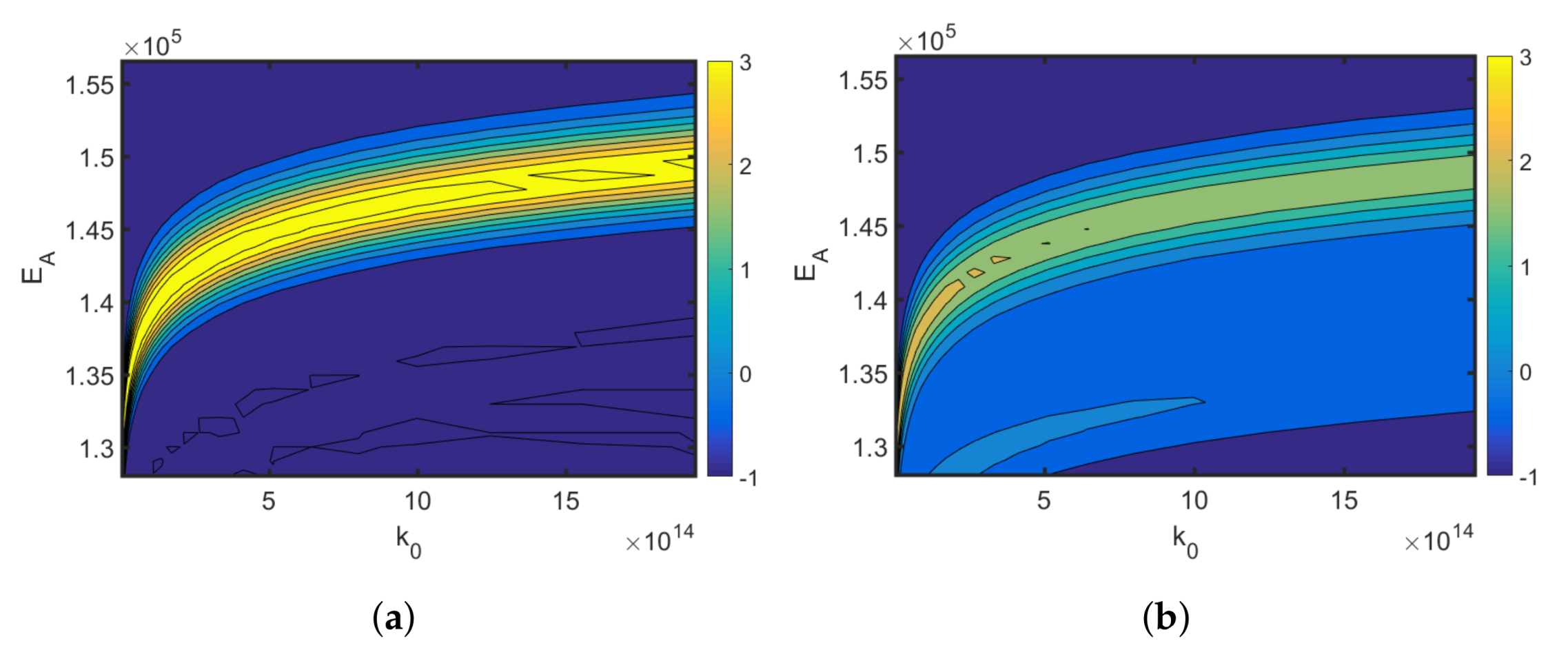
The results show that a misspecification of the applied reference Arrhenius parameters is likely to result in sub-optimal temperature profiles, less informative measurement data, and higher parameter uncertainties. Alternatively, when the multi-point averaging approach is used (Equation (8)), the calculated design is more robust against reference parameter variations; see Figure 6b. The classical D-optimality shown in Figure 6a degrades drastically with reference variations. The robust D-optimality, however, shown in Figure 6b is less affected by changing the reference parameters. As the reference parameters are typically unknown but are needed to calculate local parameter sensitivities, a robust MB-OED strategy is expected to provide more valuable MB-OED results. Moreover, global parameter sensitivities are evaluated and used for a more credible D-optimality measure (Table 4). The resulting parameter errors for the classical D-optimality, its multi-point averaging realization, and the global sensitivity-based D-design are analyzed. In Figure 7, the multi-point averaging approach and the GSA-based MB-OED lead to more precise parameter estimates in comparison to the classical D-optimality as indicated by the density functions. Here, the GSA-based design results in the most precise estimates; i.e., the probability density functions of Arrhenius parameter have their highest peak close to the true values. Moreover, the multi-point averaging approach and the GSA-based design seem to be less corrupted by the misleading second local minima of the parameter identification problem, which is indicated by the second peak of the probability density functions in Figure 7a,b. Please note, because the proposed PEM sampling strategy is used, only nine sample points for each iteration of the optimizations step are needed to calculate the multi-point averaging or GSA measures in the case of the two Arrhenius parameters.
The applied sensitivity measure has a strong impact on the MB-OED results for the Arrhenius parameters. The classical MB-OED based on local sensitivities is error-prone and is expected to provide sub-optimal experimental designs. For novel APIs, which are available only in very small quantities, each individual experimental run counts. Therefore, MB-OED following a multi-point averaging approach or GSA principles seems to be preferable. Combined with the proposed non-isothermal temperature profile strategy, the optimized temperature profiles ensure the best use of the API-scaffold DHBD and the most precise estimates of the kinetic rate parameters, and . In the next step, an MB-OED study of a more complex biochemical synthesis problem is presented where the focus is also on the effect of global design measures.
4.2. A Fed-Batch Bioreactor
In the second test case study, a fed-batch bioreactor is analyzed. A lumped version of a generic biomass-substrate model reads as follows:
where is the biomass concentration, is the substrate concentration, V is the liquid volume, and U is the inlet flow rate. The specific growth rate and the specific consumption rate follow Monod expressions
The nominal parameter values in Equations (30)–(34) and the initial conditions for the dynamic model are listed in Table 6.
For the experimental setups, the following constraints are considered. The duration of the reaction is set to 15 h. The biomass and the substrate concentration are measurable with a sample rate of 0.75 h, which results in a total set of 40 measurement samples. The maximum specific growth rate , the half velocity constant , and the yield coefficient should be estimated by minimizing the difference between the measurements and the simulation results. In this simulation study, artificial measurement data [67] are used with additive measurement noise of and for and , respectively. The MB-OED strategy aims at reducing the uncertainty of the parameters by optimizing the feeding policy of the fed-batch bioreactor. Thus, the inlet profile U is parameterized by 20 constant segments of equal size, which are optimized to provide the most informative experimental data. The Monod kinetic parameters, , and , are treated as uncertain. Their variations are expressed by uniform PDFs of different ranges, i.e., , , and , which might have been derived experimentally with a parameter identification procedure. In addition to , , and , the model parameters are assumed to be given by the literature without any uncertainty. Thus, please note that only 19 sample points for each iteration of the optimization step are needed to calculate the multi-point averaging or GSA measures when using the proposed PEM sampling strategy.
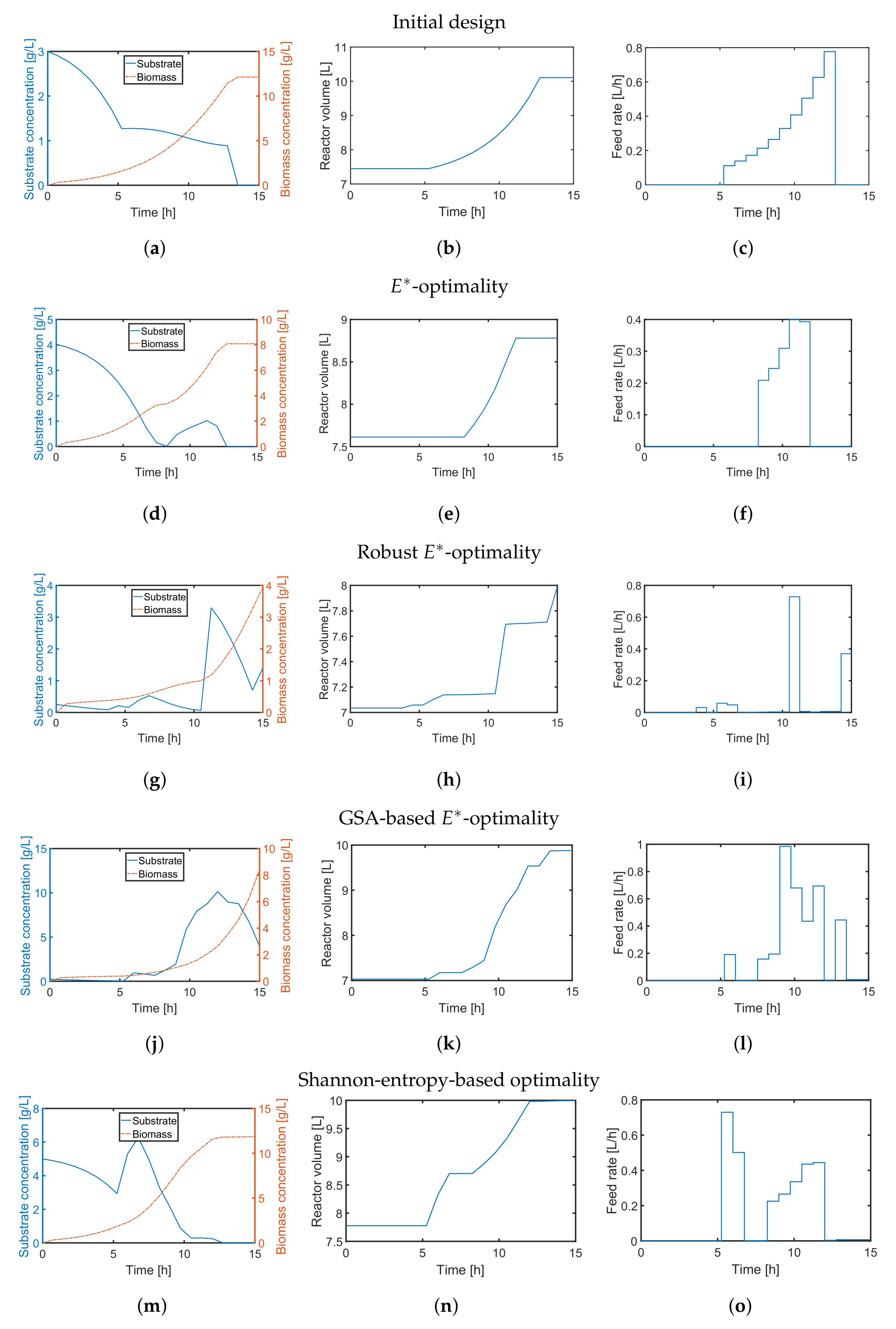
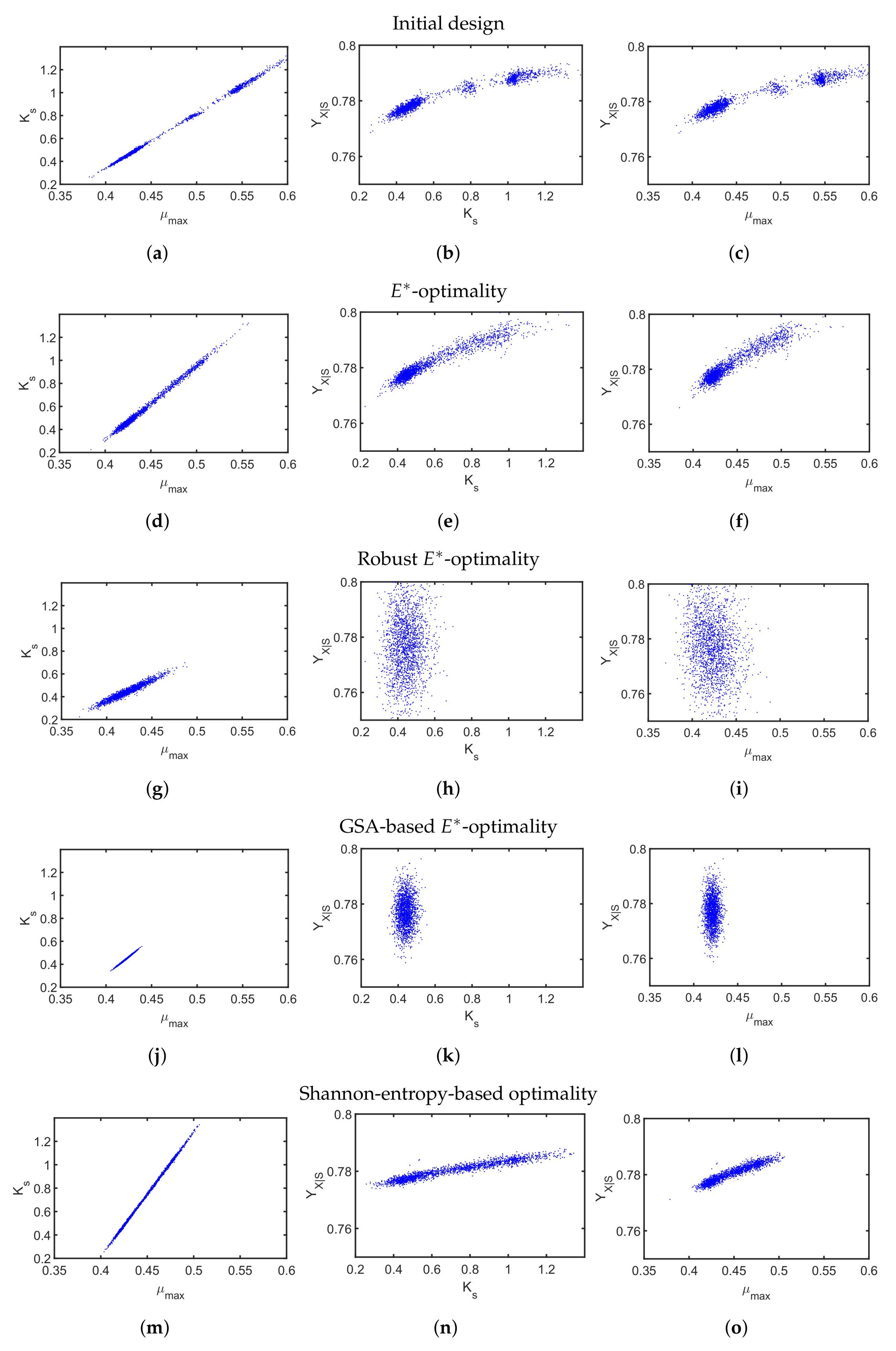
First, we applied the -design to minimize imbalanced parameter sensitivities and uncertainty. Similar to the previous case study, we compare a default substrate inlet profile (Figure 8c) with the outcome of the classical -design in Figure 8d–f. The resulting parameter scatter plots based on the initial profile (Figure 9a–c) show bimodal behavior indicating some severe nonlinearity and a non-convex optimization problem. For the classical -design, the resulting parameter variations of all three parameters (Figure 9d–f) could be only slightly improved while the parameter correlation for all parameter combinations is clearly visible. The multi-point averaging approach of the -design, in turn, seems to be more appropriate. Applying a low initial substrate concentration (Figure 8g) combined with an optimized impulse-like feeding rate (Figure 8i), the quality of the parameter estimates can be improved as illustrated in Figure 9g–i. In particular, the parameter correlations between and , and and are reduced. This effect can even be improved by implementing an MB-OED strategy based on GSA. A low initial substrate concentration (Figure 8j) but a more complex feeding rate (Figure 8l) results in more compact parameter scatter plots (Figure 9j–l); i.e., fewer parameter uncertainties and parameter correlations. Finally, in the Shannon 1 study, we also analyze the performance of a Shannon-entropy-based (Table 5) multi-objective design using as a weighting vector for
Please note that the third element was set to zero as the sum of the first-order Sobol indices () was always greater or equal to 0.9; i.e., there is no strong multivariate dependency of the analyzed parameters.
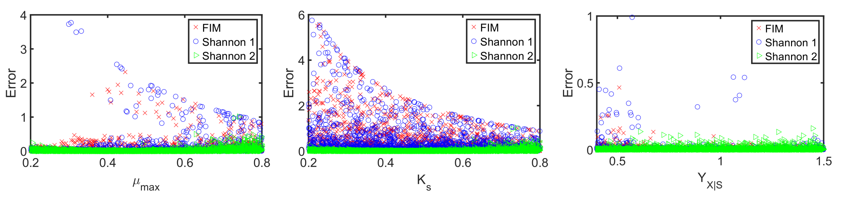
Similar to the -design, the derived initial substrate concentration is high; see Figure 8m. For the feeding rate, there are two distinct feeding periods as illustrated in Figure 8o. The resulting parameter estimates, which are summarized in Figure 9m–o, show no significant improvement in the parameter estimates in comparison to the unoptimized initial experimental setting or the -design. The main reason here is the tedious tuning of the multi-objective function, i.e., providing an optimal weighting vector w. For instance, when using in the Shannon 2 study, the quality of the parameter estimates improves significantly as illustrated in Figure 10. In comparison to the previous MB-OED results, the Shannon-entropy-based design in combination with a proper weight vector w leads to improved parameter estimates, i.e., lower parameter variations and correlations as shown in Figure 10d–f. A low initial substrate concentration (Figure 10a) followed by a gradual increase in the feeding rate (Figure 10c) provide very informative data and precise parameter estimates, respectively. This conclusion can be validated by analyzing Figure 11. The relative parameter errors clearly indicate the second Shannon-entropy-based design as the most suitable one for the parameter identification problem. Please note parameters were sampled from their assumed uniform density functions.
5. Conclusions
Without a doubt, model-based and computer-aided concepts are valuable tools for translating promising lab findings into efficient processes. Biased model-based results, however, due to model misspecification and model parameter uncertainties, are equally probable. This is particularly true when measurement data are limited in quantity and quality. Thus, in our work, we have successfully demonstrated the benefit of robustification and GSA concepts for MB-OED to gain the most informative data and to improve parameter estimates, respectively. The classical MB-OED, which is based on local sensitivities, is error-prone and is expected to provide sub-optimal experimental designs. For novel APIs, which are available only in very small quantities, each individual experimental run counts. Therefore, MB-OED following a multi-point averaging approach or GSA principles seem to be preferable as demonstrated by the DHBD synthesis problem. Moreover, Shannon-entropy-based design measures, which can account for global parameter sensitivities easily, provide a new angle in MB-OED. Assuming a proper weighting factor, it provides low parameter uncertainties and correlations as illustrated by the biochemical synthesis study.
To ensure the practical relevance, an efficient implementation of the proposed ideas was of particular interest in this study. The point estimate method framework seems to be an attractive alternative compared to state-of-the-art Monte Carlo simulations. On the one hand, it significantly reduces the computational load for advanced sensitivity analyses. On the other hand, its ease in implementation ensures a straightforward adaptation for various problems in MB-OED.
Nevertheless, there are still some open issues and potential research questions that have to be addressed in ongoing research. For instance, there is no systematic analysis under which conditions global sensitivity or robustification concepts perform best and, therefore, need to be explored in greater detail. This could lead to best-practice rules and informed decisions in MB-OED for nonlinear and complex models. An intensive study of tailored design metrics reflecting global sensitivity outcomes may also help to gain improvements in the model building process. In particular, multi-objective design concepts have to be explored and validated in the future. Finally, the proposed ideas have to be systematically extended to incorporate model misspecification as well, i.e., uncertainties related to the model structure itself in addition to the model parameters.
Acknowledgments
We acknowledge support by the German Research Foundation and the Open Access Publication Funds of the Technische Universität Braunschweig. Funding of the “Promotionsprogramm -Props” for Xiangzhong Xie and Moritz Rehbein by MWK Niedersachsen, Germany is gratefully acknowledged. Moreover, the anonymous reviewers deserve special thanks for their valuable input.
Author Contributions
R.S., X.X., and M.R. collected information and wrote the manuscript. R.S. conceived the research. X.X. performed the simulations. U.K. and S.S. provided feedback to the content and participated in writing the manuscript.
Conflicts of Interest
The authors declare no conflicts of interest.
References
- Franz, A.; Song, H.S.; Ramkrishna, D.; Kienle, A. Experimental and theoretical analysis of poly(β-hydroxybutyrate) formation and consumption in Ralstonia eutropha. Biochem. Eng. J. 2011, 55, 49–58. [Google Scholar] [CrossRef]
- Grimard, J.; Dewasme, L.; Wouwer, A.V. A review of dynamic models of hot-melt extrusion. Processes 2016, 4, 19. [Google Scholar] [CrossRef]
- Bück, A.; Neugebauer, C.; Meyer, K.; Palis, S.; Diez, E.; Kienle, A.; Heinrich, S.; Tsotsas, E. Influence of operation parameters on process stability in continuous fluidised bed layering with external product classification. Powder Technol. 2016, 300, 37–45. [Google Scholar] [CrossRef]
- Logist, F.; Erdeghem, P.V.; Smets, I.Y.; Impe, J.F.V. Multiple-objective optimisation of a jacketed tubular reactor. In Proceedings of the 2007 European Control Conference (ECC), Kos, Greece, 2–5 July 2007; pp. 963–970. [Google Scholar]
- Kunde, C.; Michaels, D.; Micovic, J.; Lutze, P.; Górak, A.; Kienle, A. Deterministic global optimization in conceptual process design of distillation and melt crystallization. Chem. Eng. Process. Process Intensif. 2016, 99, 132–142. [Google Scholar] [CrossRef]
- Kaiser, N.M.; Flassig, R.J.; Sundmacher, K. Probabilistic reactor design in the framework of elementary process functions. Comput. Chem. Eng. 2016, 94, 45–59. [Google Scholar] [CrossRef]
- Föste, H.; Schöler, M.; Majschak, J.P.; Augustin, W.; Scholl, S. Modeling and validation of the mechanism of pulsed flow cleaning. Heat Transf. Eng. 2013, 34, 753–760. [Google Scholar] [CrossRef]
- Schenkendorf, R. Supporting the shift towards continuous pharmaceutical manufacturing by condition monitoring. In Proceedings of the 2016 IEEE 3rd Conference on Control and Fault-Tolerant Systems (SysTol), Barcelona, Spain, 7–9 September 2016. [Google Scholar]
- Jelemensk, M.; Klauo, M.; Paulen, R.; Lauwers, J.; Logist, F.; Impe, J.V.; Fikar, M. Time-optimal control and parameter estimation of diafiltration processes in the presence of membrane fouling. IFAC-PapersOnLine 2016, 49, 242–247. [Google Scholar] [CrossRef]
- Rogers, A.J.; Inamdar, C.; Ierapetritou, M.G. An integrated approach to simulation of pharmaceutical processes for solid drug manufacture. Ind. Eng. Chem. Res. 2014, 53, 5128–5147. [Google Scholar] [CrossRef]
- Rantanen, J.; Khinast, J. The future of pharmaceutical manufacturing sciences. J. Pharm. Sci. 2015, 104, 3612–3638. [Google Scholar] [CrossRef] [PubMed]
- Ljung, L. System Identification: Theory for the User; Prentice-Hall: Upper Saddle River, NJ, USA, 1987. [Google Scholar]
- Balsa-Canto, E.; Alonso, A.A.; Banga, J.R. An iterative identification procedure for dynamic modeling of biochemical networks. BMC Syst. Biol. 2010, 4, 11. [Google Scholar] [CrossRef] [PubMed] [Green Version]
- Walter, E.E.; Pronzato, L. Identification of Parametric Models from Experimental Data; Springer: New York, NY, USA, 1997; p. 413. [Google Scholar]
- Rodríguez-Aragón, L.J.; López-Fidalgo, J. Optimal designs for the Arrhenius equation. Chemom. Intell. Lab. Syst. 2005, 77, 131–138. [Google Scholar] [CrossRef]
- Schenkendorf, R.; Kremling, A.; Mangold, M. Optimal experimental design with the sigma point method. IET Syst. Biol. 2009, 3, 10–23. [Google Scholar] [CrossRef] [PubMed]
- Galvanin, F.; Marchesini, R.; Barolo, M.; Bezzo, F.; Fidaleo, M. Optimal design of experiments for parameter identification in electrodialysis models. Chem. Eng. Res. Des. 2016, 105, 107–119. [Google Scholar] [CrossRef]
- Kiefer, J. Optimum experimental designs. J. R. Stat. Soc. Ser. B 1959, 21, 272–319. [Google Scholar]
- Martínez, E.C.; Cristaldi, M.D.; Grau, R.J. Design of Dynamic Experiments in Modeling for Optimization of Batch Processes. Ind. Eng. Chem. Res. 2009, 48, 3453–3465. [Google Scholar] [CrossRef]
- Sinkoe, A.; Hahn, J. Optimal experimental design for parameter estimation of an IL-6 signaling model. Processes 2017, 5, 49. [Google Scholar] [CrossRef]
- Manesso, E.; Sridharan, S.; Gunawan, R. Multi-objective optimization of experiments using curvature and Fisher information matrix. Processes 2017, 5, 63. [Google Scholar] [CrossRef]
- Chaloner, K.; Verdinelli, I. Bayesian experimental design: A review. Stat. Sci. 1995, 10, 273–304. [Google Scholar] [CrossRef]
- Gotwalt, C.M.; Jones, B.A.; Steinberg, D.M. Fast computation of designs robust to parameter uncertainty for nonlinear settings. Technometrics 2009, 51, 88–95. [Google Scholar] [CrossRef]
- Overstall, A.M.; Woods, D.C. Bayesian design of experiments using approximate coordinate exchange. Technometrics 2017, 59, 458–470. [Google Scholar] [CrossRef]
- Chu, Y.; Hahn, J. Necessary condition for applying experimental design criteria to global sensitivity analysis results. Comput. Chem. Eng. 2013, 48, 280–292. [Google Scholar] [CrossRef]
- Rodriguez-Fernandez, M.; Kucherenko, S.; Pantelides, C.; Shah, N. Optimal experimental design based on global sensitivity analysis. Comput. Aided Chem. Eng. 2007, 24, 63–68. [Google Scholar]
- Bockstal, P.J.V.; Mortier, S.; Corver, J.; Nopens, I.; Gernaey, K.V.; Beer, T.D. Global sensitivity analysis as good modelling practices tool for the identification of the most influential process parameters of the primary drying step during freeze-drying. Eur. J. Pharm. Biopharm. 2018, 123, 108–116. [Google Scholar] [CrossRef] [PubMed]
- Scire, J., Jr.; Dryer, F.; Yetter, R. Comparison of global and local sensitivity techniques for rate constants determined using complex reaction mechanisms. Int. J. Chem. Kinet. 2001, 33, 784–802. [Google Scholar] [CrossRef]
- Saltelli, A.; Ratto, M.; Tarantola, S.; Campolongo, F. Sensititivity analysis for chemical Models. Chem. Rev. 2005, 105, 2811–2828. [Google Scholar] [CrossRef] [PubMed]
- Saltelli, A.; Aleksankina, K.; Becker, W.; Fennell, P.; Ferretti, F.; Holst, N.; Sushan, L.; Wu, Q. Why so many published sensitivity analyses are false. A systematic review of sensitivity analysis practices. arXiv, 2017; arXiv:1711.11359. [Google Scholar]
- Rao, M.M.; Swift, R.J. Probability Theory with Applications; Springer: New York, NY, USA, 2006. [Google Scholar]
- Turanyi, T. Sensitivity Analysis of Complex Kinetic Systems. Tools and Applications. J. Math. Chem. 1990, 5, 203–248. [Google Scholar] [CrossRef]
- Bauer, I.; Bock, H.G.; Körkel, S.; Schlöder, J.P. Numerical methods for optimum experimental design in DAE systems. J. Comput. Appl. Math. 2010, 120, 1–25. [Google Scholar] [CrossRef]
- Ten Broeke, G.; van Voorn, G.; Kooi, B.; Molenaar, J. Detecting tipping points in ecological models with sensitivity analysis. Math. Model. Nat. Phenom. 2016, 11, 47–72. [Google Scholar] [CrossRef]
- Kucherenko, S.; Rodriguez-Fernandez, M.; Pantelides, C.; Shah, N. Monte Carlo evaluation of derivative-based global sensitivity measures. Reliab. Eng. Syst. Saf. 2009, 94, 1135–1148. [Google Scholar] [CrossRef]
- Rakovec, O.; Hill, M.C.; Clark, M.P.; Weerts, A.H.; Teuling, A.J.; Uijlenhoet, R. Distributed evaluation of local sensitivity analysis (DELSA), with application to hydrologic models. Water Resour. Res. 2014, 50, 409–426. [Google Scholar] [CrossRef]
- Zádor, J.; Zsély, I.; Turányi, T. Local and global uncertainty analysis of complex chemical kinetic systems. Reliab. Eng. Syst. Saf. 2006, 91, 1232–1240. [Google Scholar] [CrossRef]
- Iooss, B.; Lemaître, P. A review on global sensitivity analysis methods. arXiv, 2014; arXiv:1404.2405. [Google Scholar]
- Sobol, I. Global sensitivity indices for nonlinear mathematical models and their Monte Carlo estimates. Math. Comput. Simul. 2001, 55, 271–280. [Google Scholar] [CrossRef]
- Buzzard, G.T. Global sensitivity analysis using sparse grid interpolation and polynomial chaos. Reliab. Eng. Syst. Saf. 2012, 107, 82–89. [Google Scholar] [CrossRef]
- Caflisch, R.E. Monte Carlo and quasi-Monte Carlo methods. Acta Numer. 1998, 7, 1–49. [Google Scholar] [CrossRef]
- Sudret, B. Uncertainty Propagation and Sensitivity Analysis in Mechanical Models Contributions to Structural Reliability and Stochastic Spectral Methods; Habilitation a diriger des recherches; Université Blaise Pascal: Clermont-Ferrand, France, 2007. [Google Scholar]
- Tyler, G.W. Numerical integration of functions of several variables. Can. J. Math. 1953, 5, 393–412. [Google Scholar] [CrossRef]
- Lerner, U.N. Hybrid Bayesian Networks for Reasoning about Complex Systems. Ph.D. Thesis, Stanford University, Stanford, CA, USA, 2002. [Google Scholar]
- Evans, D.H. An application of numerical integration techniques to statistical tolerancing. Technometrics 1967, 9, 441–456. [Google Scholar] [CrossRef]
- Joshi, M.; Seidel-Morgenstern, A.; Kremling, A. Exploiting the bootstrap method for quantifying parameter confidence intervals in dynamical systems. Metab. Eng. 2006, 8, 447–455. [Google Scholar] [CrossRef] [PubMed]
- Heine, T.; Kawohl, M.; King, R. Derivative-free optimal experimental design. Chem. Eng. Sci. 2008, 63, 4873–4880. [Google Scholar] [CrossRef]
- Schenkendorf, R.; Mangold, M. Qualitative and quantitative optimal experimental design for parameter identification of a MAP kinase model. IFAC Proc. Vol. 2011, 44, 11666–11671. [Google Scholar] [CrossRef]
- Schenkendorf, R.; Mangold, M. Online model selection approach based on unscented Kalman filtering. J. Process Control 2013, 23, 44–57. [Google Scholar] [CrossRef]
- Franceschini, G.; Macchietto, S. Novel anticorrelation criteria for design of experiments: Algorithm and application. AIChE J. 2008, 54, 3221–3238. [Google Scholar] [CrossRef]
- Ohs, R.; Wendlandt, J.; Spiess, A.C. How graphical analysis helps interpreting optimal experimental designs for nonlinear enzyme kinetic models. AIChE J. 2017, 63, 4870–4880. [Google Scholar] [CrossRef]
- Embrechts, P.; Mcneil, A.; Straumann, D. Correlation and dependence in risk management: Properties and pitfalls. In RISK Management: Value at Risk and Beyond; Cambridge University Press: Cambridge, UK, 2002; pp. 176–223. [Google Scholar]
- Kucerová, A.; Sỳkora, J.; Janouchová, E.; Jarušková, D.; Chleboun, J. Acceleration of robust experiment design using Sobol indices and polynomial chaos expansion. In Proceedings of the 7th International Workshop on Reliable Engineering Computing (REC), Bochum, Germany, 15–17 June 2016; pp. 411–426. [Google Scholar]
- Lindley, D.V. On a measure of the information provided by an experiment. Ann. Math. Stat. 1956, 27, 986–1005. [Google Scholar] [CrossRef]
- Becker, A.; Kohfeld, S.; Lader, A.; Preu, L.; Pies, T.; Wieking, K.; Ferandin, Y.; Knockaert, M.; Meijer, L.; Kunick, C. Development of 5-benzylpaullones and paullone-9-carboxylic acid alkyl esters as selective inhibitors of mitochondrial malate dehydrogenase (mMDH). Eur. J. Med. Chem. 2010, 45, 335–342. [Google Scholar] [CrossRef] [PubMed]
- Egert-Schmidt, A.M.; Dreher, J.; Dunkel, U.; Kohfeld, S.; Preu, L.; Weber, H.; Ehlert, J.E.; Mutschler, B.; Totzke, F.; Schc̎htele, C.; et al. Identification of 2-Anilino-9-methoxy-5,7-dihydro- 6H-pyrimido[5,4-d][1]benzazepin-6-ones as Dual PLK1/VEGF-R2 Kinase Inhibitor Chemotypes by Structure-Based Lead Generation. J. Med. Chem. 2010, 53, 2433–2442. [Google Scholar] [CrossRef] [PubMed]
- Falke, H.; Chaikuad, A.; Becker, A.; Loaëc, N.; Lozach, O.; Jhaisha, S.A.; Becker, W.; Jones, P.G.; Preu, L.; Baumann, K.; et al. 10-Iodo-11H-indolo[3,2-c]quinoline-6-carboxylic Acids Are Selective Inhibitors of DYRK1A. J. Med. Chem. 2015, 58, 3131–3143. [Google Scholar] [CrossRef] [PubMed]
- Kunick, C. Fused azepinones with antitumor activity. Curr. Pharm. Des. 1999, 5, 181–194. [Google Scholar] [PubMed]
- Tolle, N.; Kunick, C. Paullones as Inhibitors of Protein Kinases. Curr. Top. Med. Chem. 2011, 11, 1320–1332. [Google Scholar] [CrossRef] [PubMed]
- Kunick, C.; Bleeker, C.; Prühs, C.; Totzke, F.; Schächtele, C.; Kubbutat, M.H.; Link, A. Matrix compare analysis discriminates subtle structural differences in a family of novel antiproliferative agents, diaryl-3-hydroxy-2,3,3a,10a-tetrahydrobenzo[b]cycylopenta[e]azepine-4,10(1H,5H)-diones. Bioorg. Med. Chem. Lett. 2006, 16, 2148–2153. [Google Scholar] [CrossRef] [PubMed]
- Rehbein, M.C.; Husmann, S.; Lechner, C.; Kunick, C.; Scholl, S. Fast and calibration free determination of first order reaction kinetics in API synthesis using in situ ATR-FTIR. Eur. J. Pharm. Biopharm. 2017, in press. [Google Scholar]
- Varga, L.; Szabó, B.; Zsély, I.G.; Zempléni, A.; Turányi, T. Numerical investigation of the uncertainty of Arrhenius parameters. J. Math. Chem. 2011, 49, 1798–1809. [Google Scholar] [CrossRef]
- Nagy, T.; Turányi, T. Uncertainty of Arrhenius parameters. Int. J. Chem. Kinet. 2011, 43, 359–378. [Google Scholar] [CrossRef]
- Schwaab, M.; Lemos, L.P.; Pinto, J.C. Optimum reference temperature for reparameterization of the Arrhenius equation. Part 1: Problems involving one kinetic constant. Chem. Eng. Sci. 2007, 63, 2750–2764. [Google Scholar] [CrossRef]
- Biegler, L.; Grossmann, I.; Westerberg, A. Systematic Methods for Chemical Process Design; Prentice Hall: Old Tappan, NJ, USA, 1997. [Google Scholar]
- Cappuyns, A.M.; Bernaerts, K.; Smets, I.Y.; Ona, O.; Prinsen, E.; Vanderleyden, J.; Van Impe, J.F. Optimal fed batch experiment design for estimation of monod kinetics of Azospirillum brasilense: From theory to practice. Biotechnol. Prog. 2007, 23, 1074–1081. [Google Scholar] [CrossRef] [PubMed]
- Telen, D.; Vercammen, D.; Logist, F.; Van Impe, J. Robustifying optimal experiment design for nonlinear, dynamic (bio)chemical systems. Comput. Chem. Eng. 2014, 71, 415–425. [Google Scholar] [CrossRef]
Figure 1.
Key elements of the model-based optimal experimental design (MB-OED): the parameter sensitivity approach and the implemented design measure determine the quality of the designed experiment significantly.
Figure 1.
Key elements of the model-based optimal experimental design (MB-OED): the parameter sensitivity approach and the implemented design measure determine the quality of the designed experiment significantly.

Figure 2.
Parameter subset selection: Starting from an unconditioned parameter sample set (a), subsets are systematically selected in (b–d) to determine conditioned expectations and variances, respectively. (a) all sample points used to calculate the unconditioned, total uncertainty ; (b) sample subsets for , , and ; (c) sample subsets for , , and ; (d) sample subsets for , , and .
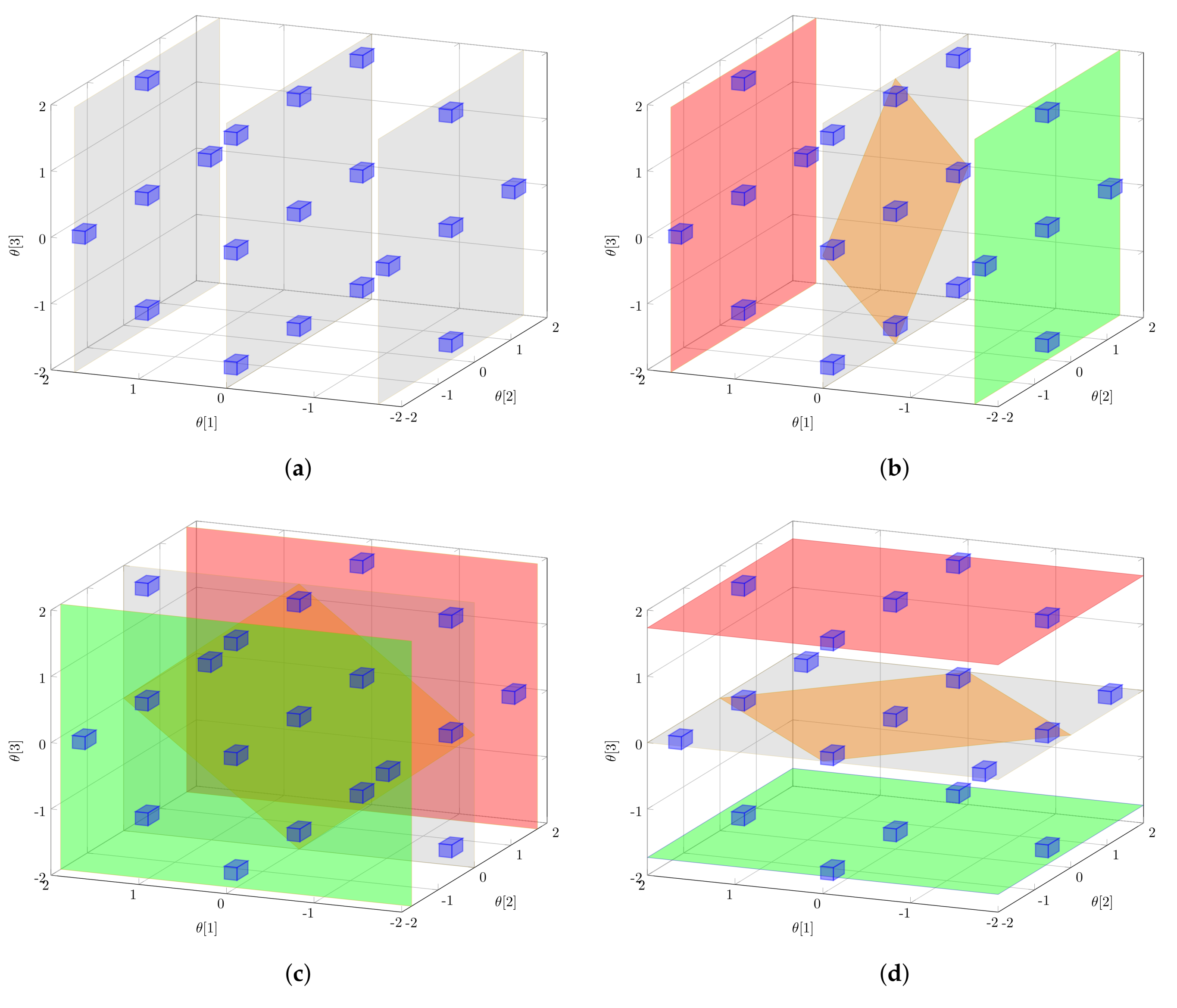
Figure 3.
Illustrative example of parameter dependencies: (a) linear correlation with ; (b) no correlation with ; and (c) nonlinear correlation but zero linear correlation (); here, eight standard Gaussian distributions are superimposed in a circular structure and properly rescaled providing a multi-modal density function. (a) linear correlated parameters; (b) linear uncorrelated parameters; (c) nonlinear correlation.

Figure 4.
Synthesis of 3,4-dihydro-1H-1-benzazepine-2,5-dione (DHBD).
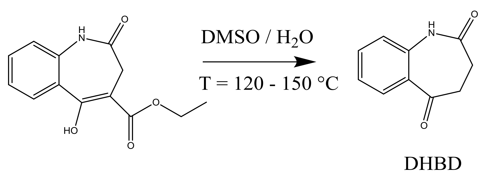
Figure 5.
Performance of the initial setting and MB-OED. D-optimality means a simplified temperature profile in comparison to D-optimality. (a) is the initial; (b) the optimally designed; and (c) the optimal but simplified temperature profile; (d–f) are the scatter plots for the estimated parameters assuming simulated noisy data for 2000 MC simulations; (g–l) are the corresponding parameter probability distributions.

Figure 6.
Effect of parameter variation. Areas close to zero mean no change in the optimized cost function (Equation (29)) when the Arrhenius parameters are changed. The classical D-optimality shown in (a) degrades drastically with parameter variations. The robust D-optimality shown in (b) is less affected by changes in the parameters. (a) D-optimality; (b) Robust D-optimality.

Figure 7.
The resulting parameter distributions of the two Arrhenius parameters for the discussed MB-OED strategies. The red circle is the reference value used for MB-OED while the blue triangle is the true parameter value. (a) Arrhenius parameter ; (b) Arrhenius parameter .
Figure 7.
The resulting parameter distributions of the two Arrhenius parameters for the discussed MB-OED strategies. The red circle is the reference value used for MB-OED while the blue triangle is the true parameter value. (a) Arrhenius parameter ; (b) Arrhenius parameter .
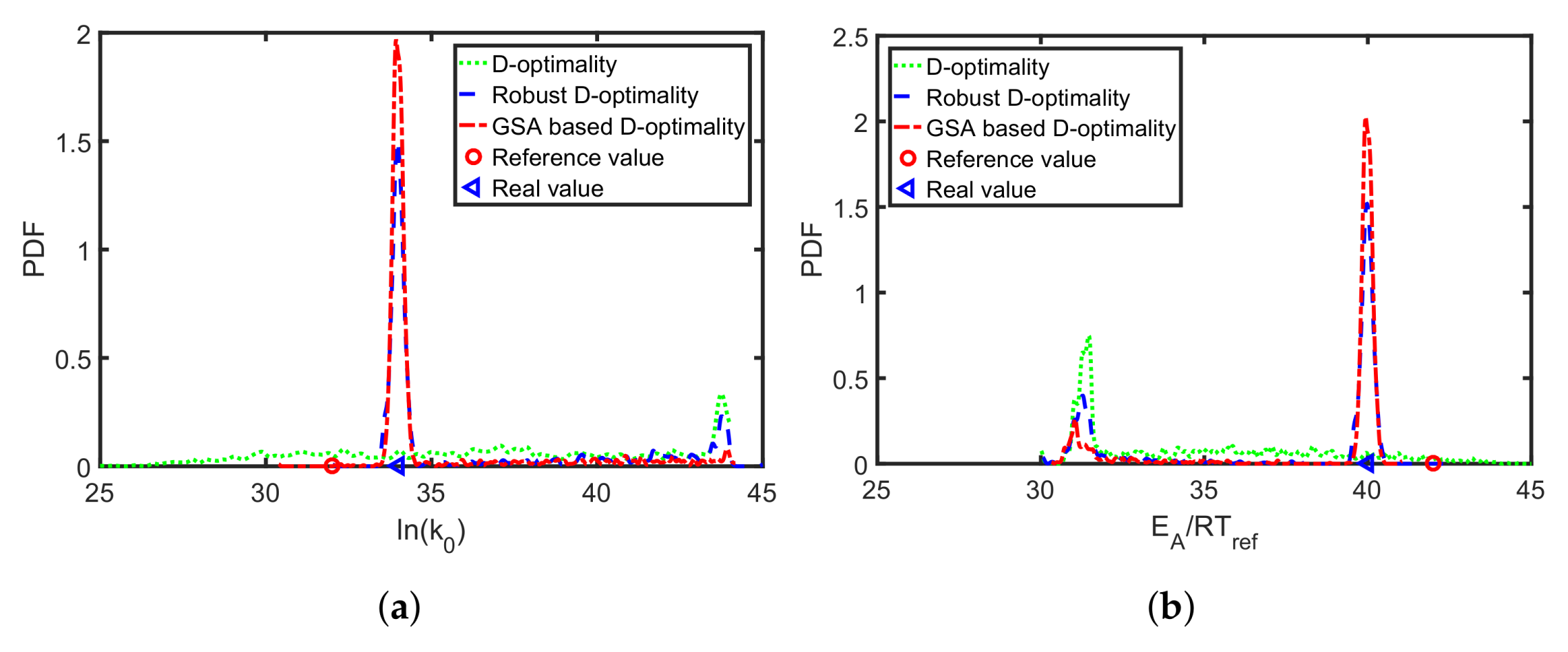
Figure 8.
MB-OED results showing the evolution of biomass and substrate concentration (left), and volume of the reactor (middle) based on the optimized feed rate (right).
Figure 8.
MB-OED results showing the evolution of biomass and substrate concentration (left), and volume of the reactor (middle) based on the optimized feed rate (right).

Figure 9.
Performance of the experiments from initial design (a–c), -optimality (d–f), robust -optimality (g–i), GSA-based -optimality (j–l), and Shannon-entropy-based design (m–o), where scatter plots are used to present the confidence region for the estimated parameters, which result from 2000 MC simulations.

Figure 10.
Evolution profiles for three states ((a) biomass concentration, substrate concentration; and (b) volume of the reactor) and (c) the feed rate for the adapted Shannon-entropy-based design with . In (d–f), the resulting parameter estimates are shown.
Figure 10.
Evolution profiles for three states ((a) biomass concentration, substrate concentration; and (b) volume of the reactor) and (c) the feed rate for the adapted Shannon-entropy-based design with . In (d–f), the resulting parameter estimates are shown.
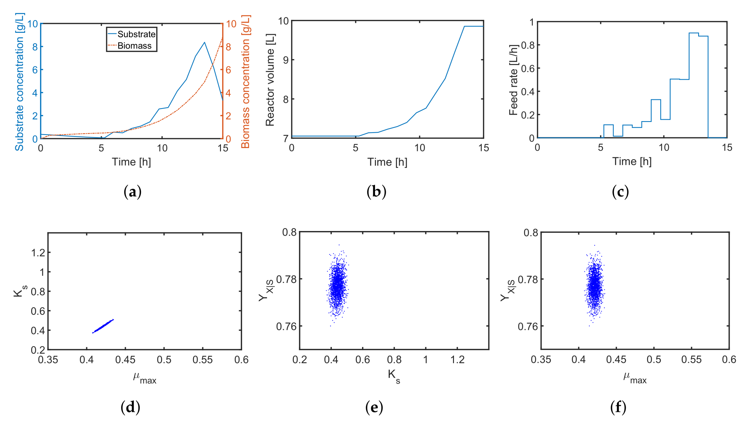
Figure 11.
Error of the parameter estimates of , and . 2000 MC simulations are shown for the classical -design and Shannon-entropy-based design with , and .
Figure 11.
Error of the parameter estimates of , and . 2000 MC simulations are shown for the classical -design and Shannon-entropy-based design with , and .

Table 1.
Statistical central moments of the standard normal (), uniform (), and triangle () distribution.
Table 1.
Statistical central moments of the standard normal (), uniform (), and triangle () distribution.
| Distribution | ||||
|---|---|---|---|---|
| 1 | 1 | 3 | 1 | |
| 1 | 1/3 | 3/5 | 1/9 | |
| 1 | 1/6 | 1/15 | 1/36 |
Table 2.
PEM parameters according to the standard normal (), uniform (), and triangle () distribution.
Table 2.
PEM parameters according to the standard normal (), uniform (), and triangle () distribution.
| Distribution | ||||
|---|---|---|---|---|
Table 3.
Local design measures for MB-OED based on the parameter covariance matrix , where refers to the modified E criterion.
Table 3.
Local design measures for MB-OED based on the parameter covariance matrix , where refers to the modified E criterion.
| Local Design Measures | Cost Functions |
|---|---|
| —optimal design | |
| —optimal design | |
| —optimal design |
Table 4.
Generalized local design measures including global sensitivities.
| GSA-Based Design Measures | Cost Functions |
|---|---|
| —optimal design | |
| —optimal design | |
| —optimal design |
Table 5.
Global design measures for MB-OED based on Sobol indices and Shannon entropy.
| Global Design Measures | Cost Function |
|---|---|
| (1) Shannon entropy (entire time horizon) | |
| (2) Shannon entropy (at single time point, ) | |
| (3) Parameter dependency | |
| (4) Overall output uncertainty |
Table 6.
Parameters as in [66] and initial conditions for the fed–batch bioreactor.
Table 6.
Parameters as in [66] and initial conditions for the fed–batch bioreactor.
| Symbol | Parameter | Unit | Nominal Value |
|---|---|---|---|
| initial concentration of biomass | 0.25 | ||
| initial concentration of substrate | 3 | ||
| initial volume of the liquid phase | 7 | ||
| substrate concentration in the feed | 50 | ||
| U | volumetric feed rate | 0–1 | |
| maximum specific growth rate | 0.421 | ||
| half velocity constant | 0.439 | ||
| yield coefficient of biomass over substrate | - | 0.777 | |
| m | maintenance factor | 0 |
© 2018 by the authors. Licensee MDPI, Basel, Switzerland. This article is an open access article distributed under the terms and conditions of the Creative Commons Attribution (CC BY) license (http://creativecommons.org/licenses/by/4.0/).
Share and Cite
MDPI and ACS Style
Schenkendorf, R.; Xie, X.; Rehbein, M.; Scholl, S.; Krewer, U. The Impact of Global Sensitivities and Design Measures in Model-Based Optimal Experimental Design. Processes 2018, 6, 27. https://doi.org/10.3390/pr6040027
AMA Style
Schenkendorf R, Xie X, Rehbein M, Scholl S, Krewer U. The Impact of Global Sensitivities and Design Measures in Model-Based Optimal Experimental Design. Processes. 2018; 6(4):27. https://doi.org/10.3390/pr6040027
Chicago/Turabian StyleSchenkendorf, René, Xiangzhong Xie, Moritz Rehbein, Stephan Scholl, and Ulrike Krewer. 2018. "The Impact of Global Sensitivities and Design Measures in Model-Based Optimal Experimental Design" Processes 6, no. 4: 27. https://doi.org/10.3390/pr6040027
Note that from the first issue of 2016, this journal uses article numbers instead of page numbers. See further details here.