Rotor-Stator Mixers: From Batch to Continuous Mode of Operation—A Review

1
Department of Food Technology, Engineering and Nutrition, Lund University, SE-221 00 Lund, Sweden
2
Department of Food and Meal Science, Kristianstad University, SE-291 88 Kristianstad, Sweden
Processes 2018, 6(4), 32; https://doi.org/10.3390/pr6040032
Submission received: 16 March 2018
/
Revised: 28 March 2018
/
Accepted: 30 March 2018
/
Published: 3 April 2018
(This article belongs to the Special Issue Feature Papers for the Fifth Year Anniversary of the Founding of Processes)
Abstract
:Although continuous production processes are often desired, many processing industries still work in batch mode due to technical limitations. Transitioning to continuous production requires an in-depth understanding of how each unit operation is affected by the shift. This contribution reviews the scientific understanding of similarities and differences between emulsification in turbulent rotor-stator mixers (also known as high-speed mixers) operated in batch and continuous mode. Rotor-stator mixers are found in many chemical processing industries, and are considered the standard tool for mixing and emulsification of high viscosity products. Since the same rotor-stator heads are often used in both modes of operation, it is sometimes assumed that transitioning from batch to continuous rotor-stator mixers is straight-forward. However, this is not always the case, as has been shown in comparative experimental studies. This review summarizes and critically compares the current understanding of differences between these two operating modes, focusing on shaft power draw, pumping power, efficiency in producing a narrow region of high intensity turbulence, and implications for product quality differences when transitioning from batch to continuous rotor-stator mixers.
1. Introduction
A fully continuous mode of production is often desired in most types of industrial processing. Continuous production decreases the per unit cost of production and reduces the risk of quality differences between batches. However, batch processing is still commonly employed in many production lines, especially in the food, pharmaceutical, and cosmetics sectors.
Continuous production does introduce some additional difficulties. The first requirement is that each unit operation in the production process can be achieved in a continuous setup. Second, converting a given batch process into a continuous one requires an understanding of what (if any) differences there are between the batch and continuous versions of each unit operation. This second difficulty also applies to product development projects for continuous mode production, since laboratory testing is almost always performed in batch.
This review focus on liquid processing in rotor-stator mixers (RSMs), also known as high-shear mixers. RSMs, together with high-pressure homogenizers, are considered the standard tool for mixing and emulsification of liquid dispersions. High-pressure homogenizers are generally used for low to intermediate viscosity products and RSMs for products with higher viscosities [1]. Whereas high-pressure homogenization is an inherently continuous operation, RSMs can be operated in either batch or continuous mode. The same rotor-stator head is often used in both batch and continuous mode of operation, see illustrations in Figure 1 and Figure 2. Continuous mode RSMs are sometimes referred to as inline (or in-line) RSMs.
From an industrial perspective, it is important to understand how the characteristics of a given batch mode RSM compare to those of a given continuous mode RSM. This understanding is crucial for both converting an existing batch production process to continuous production, and for generalizing results from laboratory (batch) experiments to pilot and production scale in a product development process. Since the rotor-stator heads are often very similar between batch and continuous modes of operation, it is tempting to assume that converting between the modes is straight-forward, both in terms of production economy (i.e., power draw of the rotor shaft) and in terms of obtained product quality (mixing or dispersing efficiency). However, as has become apparent in the scientific literature, this is not obviously the case [2,3]. Great care must therefore be taken when comparing RSMs run in batch to RSMs run in continuous mode of operation.
RSMs are used in many different applications, particularly in the food, pharmaceutical, and cosmetic processing industries. However, as pointed out in an editorial from 2001, despite their wide use, there has been a lack of fundamental understanding [4]. During the last 16 years there has been an increasing number of scientific research projects aimed at characterizing and understanding RSMs. Three major reviews have been published since then, summarizing many of these advances. In 2004, Atiemo-Obeng and Calabrese provided a comprehensive review of the mechanical designs of RSMs, focusing on power draw, flow profiles, and scale-up [5]. This review was also updated in 2016 [6]. Another fairly recent review has been provided by Zhang et al. [7], focusing on power draw and flow fields, but also providing an overview of the proposed emulsification scaling-laws and the mass and energy transfer correlations. However, none of these previous reviews provide a comprehensive discussion on the difference between batch and continuous mode of operation. Moreover, there has been a number of relevant studies on this in the last couple of years, after these reviews were written.
The objective of this contribution is to provide a more specific review on what is known about the similarities and differences between RSMs operated in batch and continuous mode, including the most recent advances. The intention is to provide an overview, both for engineering professionals struggling with the transition from batch to continuous rotor-stator mixing, and for the research community utilizing or studying RSMs. After a brief description of RSMs, this review will focus on four topics: The shaft power draw (power requirements) of batch and continuous mode RSMs (Section 3), the flowrate and pumping capacity of RSMs (Section 4), the pumping and turbulent dissipation efficiency (Section 5), and the implications of these differences on emulsion processing (Section 6). A summary of recommendations for further studies to resolve remaining issues is provided in Section 7, and the review is concluded in Section 8. Although RSMs can be operated under both laminar and turbulent conditions, this review will focus on turbulent RSMs, which are the most common RSMs employed in industrial applications.
2. The Rotor-Stator Mixer
The term RSM does not refer to a specific design but a range of mixer geometries [5]. RSMs are produced by several different manufacturers, and each have their own design, or more often several different designs for use with different applications, see References [5,7] for detailed overviews of different RSM geometries.
The common denominator of these RSMs is that they all consist of one or several high velocity rotors and one or several static stator screens separated by a short distance, the rotor-stator clearance, δ. The rotor accelerates the fluid tangentially and redirects it radially through the stator holes or slots. This gives rise to steep velocity gradients in the stator slot, or in the direct proximity of it, and creates a narrow region of high intensity hydrodynamics stresses [8,9,10,11,12,13,14,15], which give rise to high mixing and dispersing efficiency, characteristic of RSMs [14,15].
Although there are many different rotor-stator designs, they can broadly be classified into two groups based on the rotor: teeth-designs and blade-designs. A schematic view of the two design principles can be seen in Figure 3. As seen in the figure, the blade-design uses a rotor similar to that found in a centrifugal pump, either extending all the way from the shaft (as in the figure) or with shorter blades mounted on a plate attached to the rotor. The teeth-design uses a circular plate-mounted rotor, as seen in Figure 3. Both blade- and teeth-designs can use different stator screens (differing in the shape and size of the holes). Many rotor-stator heads also have multiple (i.e., 2–3) sets of concentric rotors and stators.
Figure 4 displays velocity profiles calculated with computational fluid dynamics (CFD) from two recently published investigations; one on blade-design [16] and one on teeth-design [11]. Looking at the general outline of the flow, there are many similarities. We can see how the fluid obtains a high tangential velocity in the rotor-stator clearance region, and how it is accelerated into a turbulent jet as it enters the (outer) stator slot. Note that the jet attaches to the leading edge of the stator and that the jet only fills a small portion of the slot [8,11,12]. This gives rise to a re-circulation region in the slots and, consequently, a “back-flow” of fluid that re-enters the slot from the bulk without passing the rotor [5,8,12,15,17,18].
The same rotor-stator heads are often used in both batch and continuous RSMs [3,19], the difference is primarily in how they are mounted, and how the product flow is subjected to the rotor-stator. In batch operation, the rotor-stator is mounted inside a mixing tank, either as an integrated part of the bottom of the tank as in Figure 1 (as is often the case in production-scale batch RSMs) or mounted on an impeller shaft lowered into the tank (more common for laboratory-scale batch RSMs). When used for continuous production, the rotor-stator head is mounted inside a narrow casing, similar to a centrifugal pump, with an inlet directing fluid towards the center of rotation and an outlet mounted at the periphery, see Figure 2.
3. Shaft Power Draw
The economic benefit of using an RSM depends on the power draw, Pshaft, required to operate the rotor shaft at a given speed. Much attention has been put into investigating and predicting the power draw for RSMs.
3.1. Batch Mode RSMs
A batch RSM is principally an impeller mixer, and the power draw of such systems have been under scientific investigation since the 1880s [20]. From dimensional analysis, it has been suggested that shaft power scales with rotor speed (N), rotor diameter (D), and fluid density (ρ) [21,22]:
Under turbulent conditions, the power number, NP, is constant with respect to impeller speed and diameter, but depends on tank and impeller geometry [21,22,23]. Several studies have shown that Equation (1) is valid for batch RSMs [5,7,8,10,17,24,25]. Fully turbulent, Reynolds number independent, power numbers are obtained above a critical Reynolds number of approximately 104 [24,25,26,27], with Re defined based on the rotor tip-speed:
where µ denotes fluid viscosity. The power number NP is often found to be in the range 1–3, depending on the geometry of the rotor-stator head [5,7,10,17,24,27] and the tank design [25]. These values are often found to be in the same range or somewhat lower than the power numbers of Rushton type impeller mixers [22,28].
For impeller mixers, several experimental studies have also investigated and established mathematical relations for how the impeller and tank geometry influences NP. Less information is available for batch RSMs. The tank geometry is expected to influence the power draw less than in tank agitators, since most of the pressure drop occurs in the stator. Regarding RSM geometry, several high-quality investigations have been published [17,24,25,29], but they often compare commercial designs and it has been difficult to establish which geometrical difference is responsible for the observed effects. However, there has been two recent exceptions. One study focused on the effects of stator hole width (keeping all other design parameters constant) and suggests that NP decreases with increasing stator hole diameter for a single row Tetra Pak design [10]. Another study, conducted on a range of commercial available Silverson designs, suggests that the NP is proportional to the square of the stator hole area [26]. The discrepancy between these two different systems is still not understood.
3.2. Continuous Mode RSMs
For continuous mode of operation, the power draw is more complex as the flow through the RSM is not set by the system, as in the batch case, but can be varied over a large range by the processing equipment of the continuous line. Experiments reveal that power draw depends on both rotor speed and flowrate. During the last decade several experimental investigations, using a number of different RSM designs, have found support for a three factor model that describes the power draw [7,27,30,31,32,33,34]:
where Q is the flowrate through the RSM. Equation (3) can be understood by considering that the continuous RSM is something in between a batch RSM and a centrifugal pump [5,34]. The first term, Πrot is similar to that found for the batch design, and describes the effect of rotor speed. The second term, Πflow, is similar to the power draw of a centrifugal pump and describes the effect of flowrate. The third term, ΠL is a loss-term, representing the energy lost due to vibrations and losses in bearings [33].
Equation (3) contains two constants, NP0 and NP1. Just as NP for the batch RSM, these are design dependent but do not change with flowrate or rotor speed. NP0 is often found to be on the order of 0.1 and NP1 on the order of 10. See Table 1 for specific values of these constants for a few different RSM designs. Although several studies have compared NP0 and NP1 values for different commercial designs [27,28,33,35], no systematic studies describing the effect of different design variables have yet been reported.
Although Equation (3) has received substantial experimental support, it should be remembered that RSMs can be operated under a wide set of conditions and such designs differ substantially. A correction including a fourth and a fifth term has been suggested by Jasinska et al. [16]. However, these extra terms only apply when operating the RSM at flowrates that are below what is typically used in commercial applications [16] (p. 47), and can therefore often be neglected.
Equation (3) has been used with success for describing power draw in continuous mode RSMs manufactured by Fluko [27], Silverson [28,33], Tetra Pak [35,36], and Ytron [15]. However, in one study [35], it was reported that for Conti TDS designs it is more appropriate to use a different correlation:
Note that N*P in Equation (4) is Reynolds number dependent, in contrast to NP0 and NP1 in Equation (3) [27]. It is still not completely clear why this difference is observed. The Conti design has no obvious geometrical difference when compared to the Fluko, Silverson, Tetra Pak, and Ystral mixers—for which Equation (3) is valid. The reported Conti design is with a slotted stator and a rotor with both teeth and blades [37], whereas the designs supported by Equation (3) range from teeth-designs to blades, and with a variety of different stator designs [7,28,30,31,32,33,34].
4. RSM Flowrate and Pumping
The net flowrate passing through the stator holes, Q, can be described in terms of a flow-number, NQ, via:
This applies for both batch [8,9,11,12,38] and continuous modes of operation. However, it should be noted that the interpretation and controllability of this value differ substantially between the two modes. For a continuous RSM, flowrate is an externally set and easily measured parameter. Flowrate, and consequently NQ, can be adjusted by varying what is referred to as the system curve in pump design; the total pressure loss of the system the mixer is connected to. In practice, NQ can be decreased by using a valve downstream of the mixer or increased by adding a separate feed pump placed in series with the mixer.
When the mixer is operated in batch mode, however, NQ is a constant that depends on the geometry of the mixing head [8,9,12,17,38], and to some degree on the tank geometry. The NQ parameter is important for batch RSMs since it determines how fast the liquid is mixed. More specifically the expectation value for the time a fluid element spends in the tank between two passages of the rotor-stator head is [3,19,29]:
where VT is the tank liquid volume.
Another difference between the two modes of operation is that Q (and consequently NQ) is difficult to measure for batch RSMs; it requires a non-intrusive experimental technique for measuring fluid velocities inside of and just outside of the stator slots, such as laser Doppler anemometry (LDA) [11,12,38] or particle image velocimetry (PIV) [17]. Alternatively, it can be determined by a CFD model that has been validated by one of the above-mentioned experimental techniques [17].
Table 2 compiles values of NQ for a number of different batch RSMs and compares them to the NQ span resulting from operating some different continuous mode RSMs under technically relevant flowrates [3,16,27,34,39]. As seen in Table 2, flow numbers are between 0.1 and 0.3 for batch RSMs. Systematic investigations are scarce, but based on a recent PIV investigation, it has been suggested that NQ decreases with increasing stator slot width. This phenomenon has been linked to the increase in backflow obtained when increasing the slot width [9].
For continuous RSMs, NQ is substantially lower (NQ < 0.1); it is not uncommon that continuous mode RSMs are operated at a flow number one or several decades below that of batch RSMs. This implies that the flowrates through the mixer are substantially lower for continuous mixers compared to those through batch mixers. Using the same rotor-stator head and operating it at the same rotor speed will therefore result in much lower radial velocities in the rotor-stator region. This difference can also be explained using a centrifugal pump analogy. The flowrate is determined by the properties of the pump (what in pump-theory is referred to as a pump curve) and the properties of the system (the system curve) [16]. Since tanks used with batch RSMs provide a much lower flow resistance than the pipes used for continuous RSMs, the flowrate becomes substantially higher.
5. Pumping and Turbulent Dissipation Efficiency
RSMs are designed to deliver a narrow region of high intensity shear and/or turbulence in order to achieve efficient mixing and emulsification. Under turbulent conditions, this corresponds to delivering a high local energy density or dissipation rate of turbulent kinetic energy (TKE) [13,14,16,40,41,42]. When comparing batch and continuous mode RSMs, one should therefore keep in mind that the proportion of the supplied energy which can be translated into intense turbulence differs between the two modes of operation.
5.1. Batch RSM
For a batch RSM run under turbulent conditions, all of the shaft energy (except the losses, ΠL) must ultimately be dissipated as heat. This implies that the loss-free shaft power (P’shaft) equals the total dissipated power (Pdiss):
Not all of this energy is available for mixing or emulsification since these phenomena occur in a narrow region in or around the rotor-stator head [13,40]. The energy that is dissipated outside of this high-intensity region will be an additional loss-term, seen from the point of view of the efficiency of converting energy into efficient mixing. Estimations of the local dissipation rates of TKE in a batch RSM have suggested that approximately 80% of the total dissipation occurs in the high intensity region (independent of rotor speed) for a one-row blade design [13]. This value is also close to the one reported from estimations from CFD simulations [12,17] for a similar geometry.
Assuming that the losses in bearings and those due to vibrations are negligible (ΠL/Pshaft << 1), the energy available for dispersion or mixing in a batch RSM, can be estimated directly by the power number:
Since the pump number is relatively easy to determine [33] for a given batch RSM, it is also relatively easy to estimate how much energy is available for turbulent mixing and/or emulsification in a given batch design.
5.2. Continuous Mode RSMs
It is considerably more complicated to calculate how much energy is available for generating turbulence when running an RSM in a continuous mode of operation. In this case, energy provided by the shaft can take two routes: it can either be converted to turbulent fluctuations (and subsequently dissipated as heat), Pdiss, or it can be used for pumping, Ppump. In the latter case, energy is transferred to increase the average velocity or the static pressure of the fluid, often referred to as the “head” across the RSM [35]. These effects are summarized via:
Reformulated using Equation (3):
Note the difference between the Π-terms and the P-terms in Equations (9) and (10). Πflow and Πrot are the terms used in correlations to model power draw (Equation (3)), whereas Pdiss and Ppump are the power associated with the two underlying mechanisms of turbulent dissipation and pumping. As seen below, experimental investigations reveal that the terms in the power draw correlations do not translate directly into terms in the energy balance (e.g., Πflow ≠ Pflow). Again, further insight on the continuous RSM can be gained by comparing it to a centrifugal pump, where the pumping power is proportional to the flow-term in Equation (3) (Πflow) and a linear function of the flow number [35,43]:
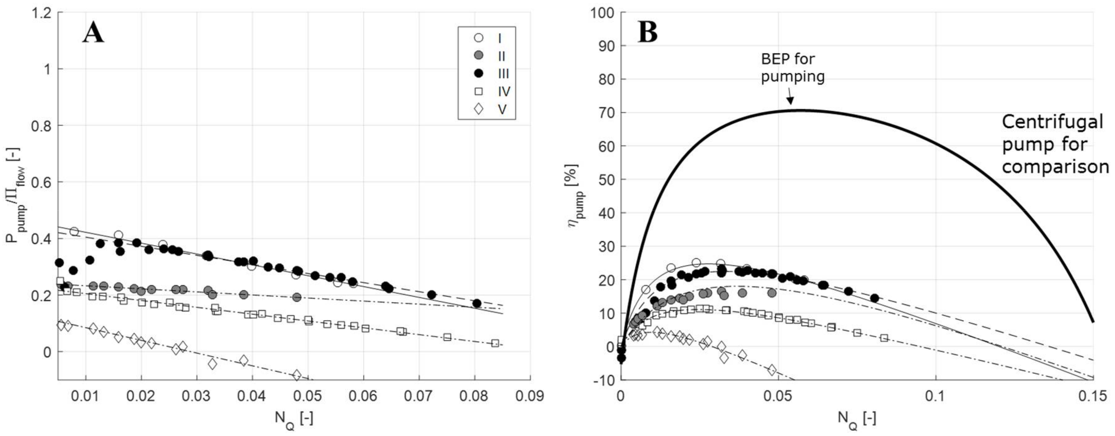
where c1 and c2 are constants that depend on the design of the centrifugal pump. A similar relation has been shown to hold true for several mixer designs [35]. Figure 5A shows the linear fit of the right-hand side parenthesis in Equation (11), used to experimentally determined the pumping powers for five continuous RSMs using data from several different investigators, RSM manufacturers, and rotor-stator head designs [27,34,36]. See Table 1 for values and design specifications.
Combining Equations (10) and (11) allows one to determine how much of the energy fed into the system is used for pumping (ηpump) and how much is dissipated as turbulence (ηturb):
Note that the efficiency is given by four empirically determined constants: the power draw constants (NP0, NP1) and the pumping constants (c1 and c2). These four constants are relatively easy to determine experimentally by measuring the power draw and the increase in head across an RSM for a range of different rotor-speeds and flowrates (see Reference [33] for the power draw methodology and Reference [35] for the pump-constant methodology).
Figure 5B shows the pumping efficiencies for the five different continuous mode RSMs from Table 1. The pumping efficiency of a centrifugal pump (LKH50, Alfa Laval, Lund, Sweden) has also been inserted as a comparison. Just as for the centrifugal pump, the percentage of energy translated into pumping in a continuous mode RSM (ηpump) varies with flowrate (NQ). For centrifugal pumps, the flowrate with the maximal pumping efficiency, often referred to as the best efficiency point (BEP) is always the desired operating point. However, for the continuous RSM, determining which flowrate is optimal will be considerably more complicated. The primary objective of the RSM is to transfer as much energy as possible into turbulence. This would suggest that a minimal ηpump (and hence a maximal ηturb) would be desired. However, continuous RSMs are often also designed to contribute to pumping the fluid; they are often used without external feed pumps. Hence, for most application a reasonable balance between pumping and turbulence efficiency is desired.
Note that the teeth-designs generally give rise to lower pumping efficiencies (see Table 1). One of the RSMs in Table 1 even gives a negative efficiency at high flowrates, implying that it is able to convert some of the power supplied from an external feed pump into turbulence. This suggest that teeth-designs are more desirable for applications where RSMs are not intended to contribute to pumping (i.e., when an external feed pump is used) and that blade-designs are more desirable for processes without an external pump.
6. Implications for Emulsification
From an industrial perspective, the most important question with regards transitioning from batch to continuous RSM is how to operate a continuous mode RSM in a way such that it results in the same product quality as batch RSM. In an emulsification context, this corresponds to the question of how to predict the resulting drop diameters in batch and continuous operation RSMs, and to the question of whether there are mechanistic differences between the two products.
Turbulent drop breakup is often explained in terms of Kolmogorov–Hinze theory [44,45,46,47,48], which suggests scaling relations between the largest drop diameter that can survive a given turbulent field and the dissipation rate of TKE of that field. Depending on the size of this limiting drop in relation to the size of the smallest turbulent structures (the Kolmogorov length-scale), different explicit scaling laws have been suggested, see References [7,41,47] for comprehensive reviews and some different explicit formulations.
However, as shown for impeller mixers [49] and high-pressure homogenizers [50], in order for this approach to be satisfactory, the dissipation rate of turbulent kinetic energy should be the local value in the most intense region (where breakup takes place). However, since the local dissipation rate of TKE is highly challenging to measure [49], practical application of Kolmogorov–Hinze theory to RSMs are often based on externally measurable quantities such as rotor speed [31,39,51], the total dissipation power (Pdiss) [52,53], and the globally defined Reynolds and Weber numbers [41]. The global Weber number is defined as:
where σ is the interfacial tension of the drop. The Kolmogorov–Hinze theory is very general, and not specific to design or mode of operation. However, there is some disagreement in the scientific literature when it comes to the question of if there are mechanistic differences between emulsification in the two modes of operation, and hence, if the same scaling law expressions can be used for both modes of operation.
Experimental studies have reported some systematic differences. Emulsions passed n times through a batch RSM do not always show the same drop size as an emulsion processed for a time t = nτ, despite the fact that this would result in the same the number of passages though the RSM, at least in terms of expectation number [2,3]. Three different standpoints discussing this discrepancy and the emulsification implications can be found in the RSM literature.
6.1. Flowrate and Its Influence on Turbulence
As previously mentioned, there is a decisive difference in flowrate (and thus in NQ) between RSMs operated in batch and continuous mode; batch mode RSMs show approximately ten times higher flowrates (Table 2). The difference between the two systems can be investigated by understanding the effect of flowrate on emulsification. Hall et al. [39] undertook a large systematic investigation of emulsification in continuous mode RSMs and suggested that the flowrate-based Reynold number:
where d is the slot diameter and Atot is the total flow-through area of the stator, has a small but significant effect on the resulting drop size (when tip-speed is kept constant). When keeping the geometry constant, it can be shown that ReQ is proportional to the product between flow number and Reynolds number [54]:
This would suggest that NQRe would be an appropriate scaling law when comparing emulsification results from batch to inline mode of operation. However, it should be kept in mind that the variations in flowrate seen in this type of experiment are much smaller than that between continuous and batch RSMs.
6.2. Radial Flow and Dissiaption Profile Scaling
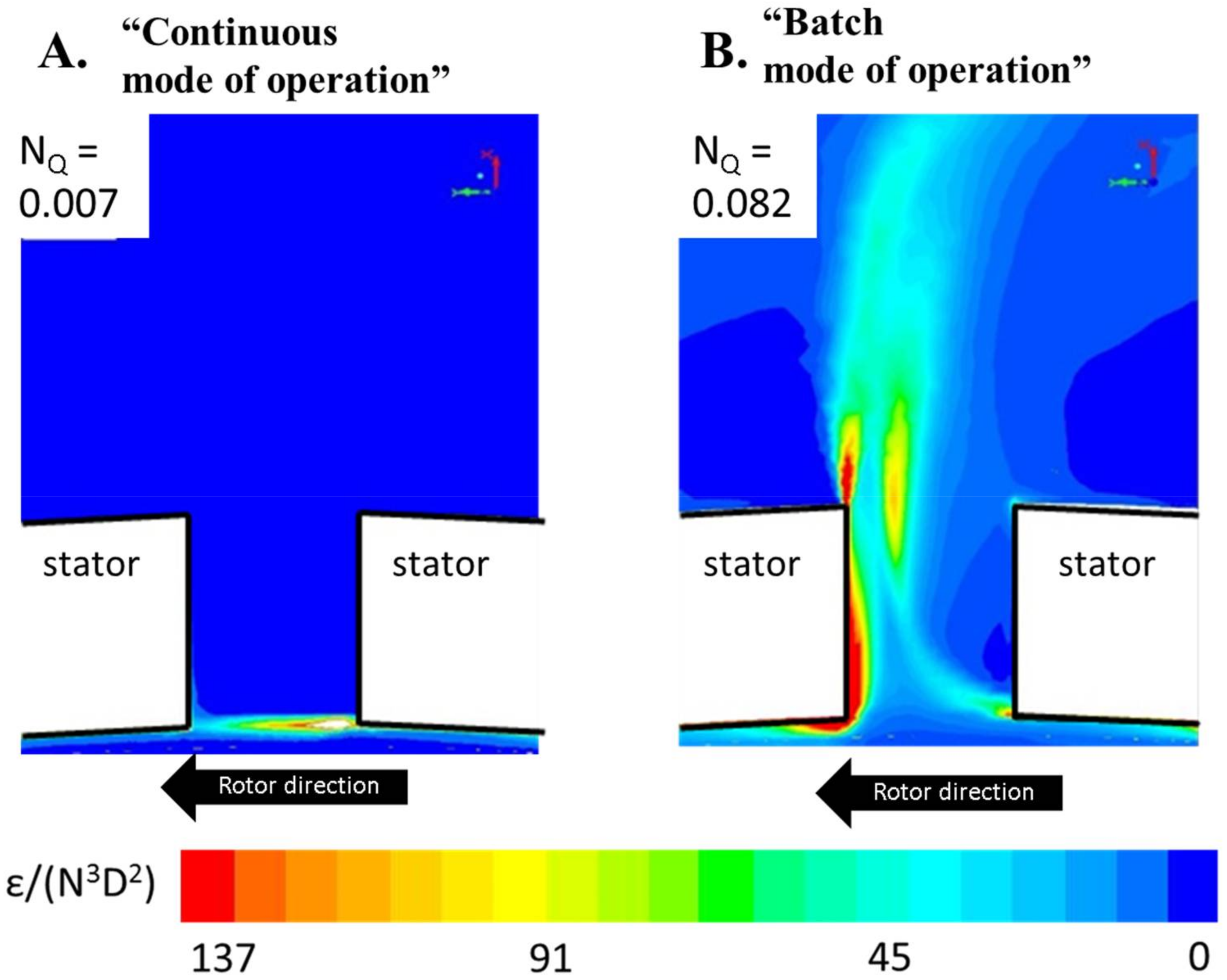
RSM mixing and emulsification ultimately depends on the hydrodynamic conditions created in the rotor-stator region. Thus, it is interesting to investigate if there are any differences to the flow fields between batch and continuous modes of operation for the same rotor speed and rotor-stator head geometry. Unfortunately, no such experimental studies have been reported. However, a recent CFD investigation might be used to shed some light on the situation [54]. The study [54] reports flow fields obtained with CFD for a continuous mode RSM run at different flowrates and rotor speeds. The lower flowrates correspond to those generally obtained for continuous mode of operation (NQ = 0.007) and the higher to those obtained in batch mode of operation (NQ = 0.082). The radial velocity profiles in the stator holes were compared and it was found that neither ReQ nor NQReQ were appropriate scaling laws, in contrast to what was suggested in Section 6.1. Instead, it was found that both radial and tangential velocities (appropriately scaled with rotor speed) were determined by the flow number [54]. This has an important implication on the difference between the two modes of operation. Since transitioning from batch RSM to a continuous mode RSM decreases NQ, the velocity profile in the rotor-stator head will undergo a substantial change. This change is not merely a scaling due to the reduction in flowrate but a shift into a fundamentally different turbulent flow [54]. Most notably the position of the highest local dissipation rate of TKE shifts from the turbulent jet formed downstream of the slot in the batch RSM flow number, to the rotor-stator clearance for the continuous RSM flow numbers [54]. This effect is illustrated in Figure 6.
A shift in the position of highest local dissipation rate of TKE suggests a mechanistic difference between the two modes of operation. As seen in Figure 6, the dissipation volume is smaller for the low-NQ (continuous mode) case than in the high-NQ (batch mode) case. This also suggests that the average dissipation rate in the two regions will scale with different parameters: with the clearance length-scale for continuous RSMs and with the slot diameter for the batch RSM. However, this has not yet been experimentally verified.
Due to the lack of experimentally measured flow fields, this difference in flow pattern between modes of operation has not yet been experimentally verified, but a validation study has shown that the CFD model employed is able to capture the position of high intensity local dissipation at least for the batch RSM [55].
Further insight can be obtained by single drop breakup visualizations. However, only one such study on RSMs has yet been reported [42]. This study was conducted for a batch RSM (NQ = 0.11) [8] and showed that drops are deformed and subsequently broken up just downstream of the stator hole [42], as suggested by the CFD simulations for the NQ-values found in batch RSM (i.e., in Figure 6). However, no corresponding investigations on continuous RSMs (or low NQ-systems) have yet been reported.
6.3. A Purely Stochastic Effect
An altogether different, but highly promising approach to describe the previously reported differences between batch and continuous modes of operation on emulsification results has recently been reported. Carrillo De Hert and Rodgers [19] suggest that the differences only apply if the wrong scaling is employed when comparing data from different modes of operation.
In the first step of their study, they conclude that the mode drop diameter, d0, resulting from processing an emulsion n times through their continuous mode RSM at flowrate Q and rotor speed N is given by [19]:
Note the −6/5 exponent, that corresponds to the scaling expected from Kolmogorov–Hinze breakup in the turbulent viscous regime [7,47].
The authors then continue by suggesting that the only difference between continuous and batch modes of operation is in the stochastic effect of the rotor-stator head passage [19]. After processing an emulsion for a time t in a batch system, the expectation number of the number of passages is:
However, for each volume element of the emulsion, the actual number of passages is a stochastic property following a Poisson distribution. By assuming that Equation (16) (the model for continuous mode of operation) applies each time a volume element passes the rotor-stator head, they conclude that the corresponding model for a batch system after being processed for a time t would be [19]:
Moreover, for t/τ > 2, Equation (18) converges to [19]:
which was found to accurately describe their data for a wide range of properties [19].
These results suggest that there is no mechanistic difference between the modes of operation and that (at least when processing times are fairly large) emulsification results can be translated directly using Equation (17); one continuous mode RSM passage would then correspond directly to processing for t/τ in a batch RSM. However, this is not completely general. In a previous study on emulsification of mayonnaise, it was concluded that this scaling was inadequate to describe the experimental differences [3]. The reason behind this discrepancy is still not understood, but it is hypothesized that it is related to the higher volume fraction of oil in Reference [3] which increases the complexity of the process.
In summary, there is as of yet no consensus in literature on which (if any) of these theories (Section 6.1, Section 6.2 and Section 6.3) best describes the differences between emulsification efficiency in batch and continuous modes of operation. Some of the confusion can be explained by postulating that the underlying differences between batch and continuous modes—i.e., the higher flowrate in batch systems—are the different hydrodynamic effects of the rotor-stator head in RSMs with different designs. It might be that the ReQ-scaling is appropriate for the design investigated by Hall et al. [39] (a pilot scale Silverson dual blade design), that the NQ-scaling is appropriate for the design investigated by Håkansson et al. [54] (a production scale Tetra Pak blade design), and that there is no mechanistic difference for the design investigated by Carrillo De Hert and Rodgers [19] (a laboratory scale Silverson blade design). However, it is not clear why these different behaviors would occur, and how they could be linked to the design differences. Further investigations are needed in order to draw any definite conclusions on this matter.
7. Suggestion for Further Research
During the last couple of years, significant advances have been made into improving the fundamental understanding of RSMs in general and more specifically on the difference between batch and continuous modes of operation. However, there are still a number of issues that need further investigation, especially when it comes to the difference between continuous and batch modes of operation:
- Although general models for the scaling of power draw with operating parameters have now been obtained for both modes of operation (Equations (1) and (3)), there is still a lack of systematic investigation into how the model parameters (NP, NP0, NP1) depend on the design parameters (rotor, stator and tank dimensions). A better understanding of this would be helpful in the mechanical design of both batch and continuous mode RSMs.
- As seen throughout this review, the continuous mode RSM could be seen as something between a batch RSM and a centrifugal pump. Further investigations on the relative pumping and turbulence producing properties of different mixer designs (i.e., determination of pumping constants, c1 and c2) would be helpful for choosing the right rotor-stator head for a given application.
- A large number of experimental studies correlating drop sizes to operating parameters have been published, but it has been difficult to use these studies to obtain a fundamental understanding of the breakup process or the underlying hydrodynamics of RSMs. The single drop breakup visualizations reported by Ashar et al. [42] shows a promising alternative approach where the breakup probabilities are measured directly and then linked to the local hydrodynamic conditions. Expanding these types of investigations into other RSM geometries and repeating it for a continuous mode RSM is needed to further our fundamental understanding.
- As seen in Section 6, there is some remaining uncertainty whether there exist mechanistic differences between breakup when using the same rotor-stator head in the batch or continuous mode of operation. Comparing the scaling suggested by Carrillo De Hert and Rodgers [19] to data from more RSM designs could be one way towards reaching a more definite conclusion; single drop breakup visualization in a continuous mode RSM at varying NQ-values would be another interesting way forward.
8. Summary and Conclusions
The objective of this contribution was to review the current scientific based understanding of the differences between RSMs in batch or continuous mode of operation. Section 3 showed that correlations for shaft power draw are available for both modes of operation, allowing for accurate prediction of process economy in terms of energy expenditure. In Section 4, it was seen that the flow number (NQ), and consequently the flow through the stator screen, Q, is considerably lower for continuous mode of operation (compared to batch mode) when using the same rotor-stator head and operating it at the same rotor speed. Section 5 showed that, in general, a much higher proportion of the energy fed to the shaft is converted into turbulence in the high-intensity region where mixing and emulsification takes place for a batch RSM than for an RSM operated in continuous mode. For a continuous mode RSM, more of the energy is used for pumping (i.e., increasing the head of the flow). Section 6 discussed what this implies when comparing emulsification efficiencies between the two modes of operation. Several different theories have been suggested, but there is of yet no clear consensus in the literature for how continuous mode RSMs should be operated in order to give the same emulsion as in a batch RSM.
Acknowledgments
This study received no external funding. Fredrik Innings at Lund University is acknowledged for valuable discussion and insightful comments on an earlier draft of the manuscript.
Conflicts of Interest
The author declares no conflict of interest.
References
- Schultz, S.; Wagner, G.; Urban, K.; Ulrich, J. High-pressure homogenization as a process for emulsification. Chem. Eng. Technol. 2004, 27, 361–368. [Google Scholar] [CrossRef]
- Bourne, J.R.; Studer, M. Fast reactions in rotor-stator mixers of different size. Chem. Eng. Process. 1992, 31, 285–296. [Google Scholar] [CrossRef]
- Håkansson, A.; Chaudhry, Z.; Innings, F. Model emulsions to study the mechanism of industrial mayonnaise emulsification. Food Bioprod. Process. 2016, 98, 189–195. [Google Scholar] [CrossRef]
- Calabrese, R. Research needs and opportunities in fluid mixing technology. Chem. Eng. Res. Des. 2001, 79, 111–112. [Google Scholar] [CrossRef]
- Atiemo-Obeng, V.A.; Calabrese, R. Rotor-stator mixing devices. In Handbook of Industrial Mixing; Paul, E.L., Atiemo-Obeng, V.A., Kresta, S.M., Eds.; Wiley: Hoboken, NJ, USA, 2004; pp. 479–505. [Google Scholar]
- Atiemo-Obeng, V.A.; Calabrese, R. Rotor-stator mixing devices. In Advances in Industrial Mixing; Kresta, S.M., Etchells, A.W., Dickey, D.S., Atiemo-Obeng, V.A., Eds.; Wiley: Hoboken, NJ, USA, 2016; pp. 255–258. [Google Scholar]
- Zhang, J.; Xu, S.; Li, W. High shear mixers: A review of typical applications and studies on power draw, slot pattern, energy dissipation and transfer properties. Chem. Eng. Process. 2012, 57–58, 25–41. [Google Scholar] [CrossRef]
- Mortensen, H.H.; Calabrese, R.V.; Innings, F.; Rosendahl, L. Characteristics of a batch rotor-stator mixer performance elucidated by shaft torque and angle resolved PIV measurements. Can. J. Chem. Eng. 2011, 89, 1076–1095. [Google Scholar] [CrossRef]
- Mortensen, H.H.; Innings, F.; Håkansson, A. The effect of stator design on flowrate and velocity fields in a rotor-stator mixer—An experimental investigation. Chem. Eng. Res. Des. 2017, 121, 245–254. [Google Scholar] [CrossRef]
- Mortensen, H.H.; Innings, F.; Håkansson, A. Local levels of dissipation rate of turbulent kinetic energy in a rotor-stator mixer with different stator slot widths—An experimental investigation. Chem. Eng. Res. Des. 2018, 130, 52–62. [Google Scholar] [CrossRef]
- Xu, S.; Cheng, Q.; Li, W.; Zhang, J. LDA Measurements and CFD simulations of an in-line high shear mixer with ultrafine teeth. AIChE J. 2014, 60, 1143–1155. [Google Scholar] [CrossRef]
- Utomo, A.; Baker, M.; Pacek, A.W. Flow pattern, periodicity and energy dissipation in a batch rotor-stator mixer. Chem. Eng. Res. Des. 2008, 89, 1397–1409. [Google Scholar] [CrossRef]
- Håkansson, A.; Mortensen, H.H.; Andersson, R.; Innings, F. Experimental investigations of turbulent fragmenting stresses in a Rotor-Stator Mixer. Part 1. Estimation of turbulent stresses and comparison to breakup visualizations. Chem. Eng. Sci. 2017, 171, 625–637. [Google Scholar] [CrossRef]
- Jasinska, M.; Baldyga, J.; Hall, S.; Pacek, A.W. Dispersion of oil droplets in rotor-stator mixers: Experimental investigations and modelling. Chem. Eng. Process. 2014, 84, 45–53. [Google Scholar] [CrossRef]
- Özcan-Taskin, G.; Kubicki, D.; Padron, G. Power and flow characteristics of three rotor-stator heads. Can. J. Chem. Eng. 2011, 89, 1005–1017. [Google Scholar] [CrossRef]
- Jasinska, M.; Baldyga, J.; Cooke, M.; Kowalski, A.J. Specific features of power characteristics of in-line rotor-stator mixers. Chem. Eng. Process. 2015, 9, 143–159. [Google Scholar] [CrossRef]
- Utomo, A.; Baker, M.; Pacek, A.W. The effect of stator geometry on the flow pattern and energy dissipation rate in a rotor-stator mixer. Chem. Eng. Res. Des. 2009, 87, 533–542. [Google Scholar] [CrossRef]
- Espinoza, C.J.U.; Simmons, M.J.H.; Albertini, F.; Mihailova, O.; Rothman, D.; Kowalski, A.J. Flow studies in an in-line Silverson 150/250 high shear mixer using PIV. Chem. Eng. Res. Des. 2018, 132, 989–1004. [Google Scholar] [CrossRef]
- Carrillo De Hert, S.; Rodgers, T.L. Continuous, recycle and batch emulsification kinetics using a high-shear mixer. Chem. Eng. Sci. 2017, 167, 265–277. [Google Scholar] [CrossRef]
- Unwin, W.C. On the friction of water against solid surfaces of different degrees of roughness. Proc. R. Soc. Lond. 1880, 31, 54–58. [Google Scholar] [CrossRef]
- White, A.M.; Brenner, E. Studies in agitation vs. the correlation of power data. Trans. Am. Inst. Chem. Eng. 1934, 30, 555–597. [Google Scholar]
- Rushton, J.H.; Costich, E.W.; Everett, H.J. Power characteristics of mixing impellers. Part 1. Chem. Eng. Prog. 1950, 46, 395–404. [Google Scholar]
- Bates, R.L.; Fondy, P.L.; Corpstein, R.R. An examination of some geometric parameters of impeller power. Ind. Eng. Chem. Process Des. Dev. 1963, 2, 310–314. [Google Scholar] [CrossRef]
- Padron, G.A. Measurement and Comparison of Power Draw in Batch Rotor-Stator Mixers. Master’s Thesis, University of Maryland, College Park, MD, USA, 2001. [Google Scholar]
- Myers, K.J.; Reeder, M.F.; Ryan, D. Power draw of a high-shear homogenizer. Can. J. Chem. Eng. 2001, 79, 94–99. [Google Scholar] [CrossRef]
- James, J.; Cooke, M.; Trinh, L.; Hou, R.; Martin, P.; Kowalski, A.; Rodgers, T.L. Scale-up of batch rotor-stator mixers. Part 1–Power constants. Chem. Eng. Res. Des. 2017, 124, 313–320. [Google Scholar] [CrossRef]
- Cheng, Q.; Xu, S.; Shi, J.; Li, W.; Zhang, J. Pump capacity and power consumption of two commercial in-line high shear mixers. Ind. Eng. Chem. Res. 2012, 52, 525–537. [Google Scholar] [CrossRef]
- Cooke, M.; Rodgers, T.L.; Kowalski, A.J. Power consumption characteristics of an in-line Silverson high shear mixer. AIChE J. 2012, 58, 1683–1692. [Google Scholar] [CrossRef]
- Nienow, A.W. On impeller circulation and mixing effectiveness in the turbulent flow regime. Chem. Eng. Sci. 1997, 52, 2257–2565. [Google Scholar] [CrossRef]
- Baldyga, J.A.; Kowalski, A.J.; Cooke, M.; Jasinska, M. Investigations of micromixing in the rotor-stator mixer. Chem. Process Eng. 2007, 28, 867–877. [Google Scholar]
- Hall, S.; Pacek, A.W.; Kowalski, A.J.; Cooke, M.; Rothman, D. The effect of scale and interfacial tension on liquid–liquid dispersion in-line Silverson rotor-stator mixers. Chem. Eng. Res. Des. 2013, 91, 2156–2168. [Google Scholar]
- Kowalski, A.J. Power consumption of in-line rotor-stator devices. Chem. Eng. Process. 2009, 48, 581–585. [Google Scholar] [CrossRef]
- Kowalski, A.J.; Cooke, M.; Hall, S. Expression for turbulent power draw of an inline Silverson high shear mixer. Chem. Eng. Sci. 2011, 66, 241–249. [Google Scholar] [CrossRef]
- Sparks, T. Fluid Mixing in Rotor/Stator Mixers. Ph.D. Thesis, Cranfield University, Cranfield, UK, 1996. [Google Scholar]
- Håkansson, A.; Innings, F. The dissipation rate of turbulent kinetic energy and its relation to pumping power in inline rotor-stator mixers. Chem. Eng. Process. 2017, 115, 46–55. [Google Scholar] [CrossRef]
- Lindahl, A. Fluid Dynamics of Rotor Stator Mixers. Master’s Thesis, Luleå University, Luleå, Sweden, 2013. [Google Scholar]
- Schönstedt, B.; Jacob, H.-J.; Schilde, C.; Kwade, A. Scale-up of the power draw of inline-rotor-stator mixers with high throughput. Chem. Eng. Res. Des. 2015, 93, 12–20. [Google Scholar] [CrossRef]
- Pacek, A.; Baker, M.; Utomo, A.T. Characterisation of flow pattern in a rotor stator high shear mixer. In Proceedings of the European Congress of Chemical Engineering, Copenhagen, Denmark, 16–20 September 2007. [Google Scholar]
- Hall, S.; Cooke, M.; Pacek, A.W.; Kowalski, A.J.; Rothman, D. Scaling up of silverson rotor-stator mixers. Can. J. Chem. Eng. 2011, 89, 1040–1050. [Google Scholar] [CrossRef]
- Jasinska, M.; Baldyga, J.; Cooke, M.; Kowalski, A. Application of test reactions to study micromixing in the rotor-stator mixer (test reactions for rotor-stator mixer). Appl. Therm. Eng. 2013, 57, 172–179. [Google Scholar] [CrossRef]
- Rueger, P.E.; Calabrese, R.V. Dispersion of water into oil in a rotor-stator mixer. Part 1: Drop breakup in dilute systems. Chem. Eng. Res. Des. 2013, 91, 2122–2133. [Google Scholar] [CrossRef]
- Ashar, M.; Arlov, D.; Carlsson, F.; Innings, F.; Andersson, R. Single droplet breakup in a rotor-stator mixer. Chem. Eng. Sci. 2018, 181, 186–198. [Google Scholar] [CrossRef]
- White, F. Fluid Mechanics, 4th ed.; McGraw-Hill: Boston, MA, USA, 1998; ISBN 0070697167. [Google Scholar]
- Kolmogorov, A.N. On the breakage of drops in a turbulent flow. Dokl. Akad. Nauk. SSSR 1949, 66, 825–828. [Google Scholar]
- Hinze, J.O. Fundamentals of the Hydrodynamic Mechanism of Splitting in dispersion processing. AIChE J. 1955, 1, 289–295. [Google Scholar] [CrossRef]
- Davies, J.T. Drop sizes of emulsions related to turbulent energy dissipation rates. Chem. Eng. Sci. 1985, 40, 839–842. [Google Scholar] [CrossRef]
- Vankova, N.; Tcholakova, S.; Denkov, N.D.; Ivanov, I.B.; Vulchev, V.D.; Danner, T. Emulsification in turbulent flow 1. Mean and maximum drop diameters in inertial and viscous regimes. J. Colloid Interface Sci. 2007, 312, 363–380. [Google Scholar] [CrossRef] [PubMed]
- Walstra, P. Emulsions. In Fundamentals of Interface and Colloid Science; Lyklema, J., Ed.; Elsevier: Amsterdam, The Netherland, 2005; Volume 5, pp. 1–94. ISBN 9780124605305. [Google Scholar]
- Zhou, G.; Kresta, S.M. Correlation of mean drop size and minimum drop size with the turbulence energy dissipation and the flow in an agitated tank. Chem. Eng. Sci. 1998, 53, 2063–2079. [Google Scholar] [CrossRef]
- Håkansson, A.; Fuchs, L.; Innings, F.; Revstedt, J.; Trägårdh, C.; Bergenståhl, B. High resolution experimental measurement of turbulent flow field in a high pressure homogenizer model and its implications on turbulent drop fragmentation. Chem. Eng. Sci. 2011, 66, 1790–1801. [Google Scholar] [CrossRef]
- Hall, S.; Cooke, M.; El-Hamouz, A.; Kowalski, A.J. Droplet break-up by in-line Silverson rotor-stator mixer. Chem. Eng. Sci. 2011, 66, 2068–2079. [Google Scholar] [CrossRef]
- Karbstein, H.; Schubert, H. Developments in the continuous mechanical production of oil-in-water macro-emulsions. Chem. Eng. Process. 1995, 34, 205–211. [Google Scholar] [CrossRef]
- Rodgers, T.L.; Cooke, M. Rotor-stator devices: The role of shear and the stator. Chem. Eng. Res. Des. 2012, 90, 323–327. [Google Scholar] [CrossRef]
- Håkansson, A.; Arlov, D.; Carlsson, F.; Innings, F. Hydrodynamic difference between inline and batch operation of a rotor-stator mixer head—A CFD approach. Can. J. Chem. Eng. 2017, 95, 806–816. [Google Scholar] [CrossRef]
- Mortensen, H.H.; Arlov, D.; Innings, F.; Håkansson, A. A validation of commonly used CFD methods applied to Rotor Stator Mixers using PIV measurements of fluid velocity and turbulence. Chem. Eng. Sci. 2018, 177, 340–353. [Google Scholar] [CrossRef]
Figure 1.
Schematic drawings of rotor-stator mixers (RSMs) operated in continuous (A) and batch (B) mode of operation.
Figure 1.
Schematic drawings of rotor-stator mixers (RSMs) operated in continuous (A) and batch (B) mode of operation.
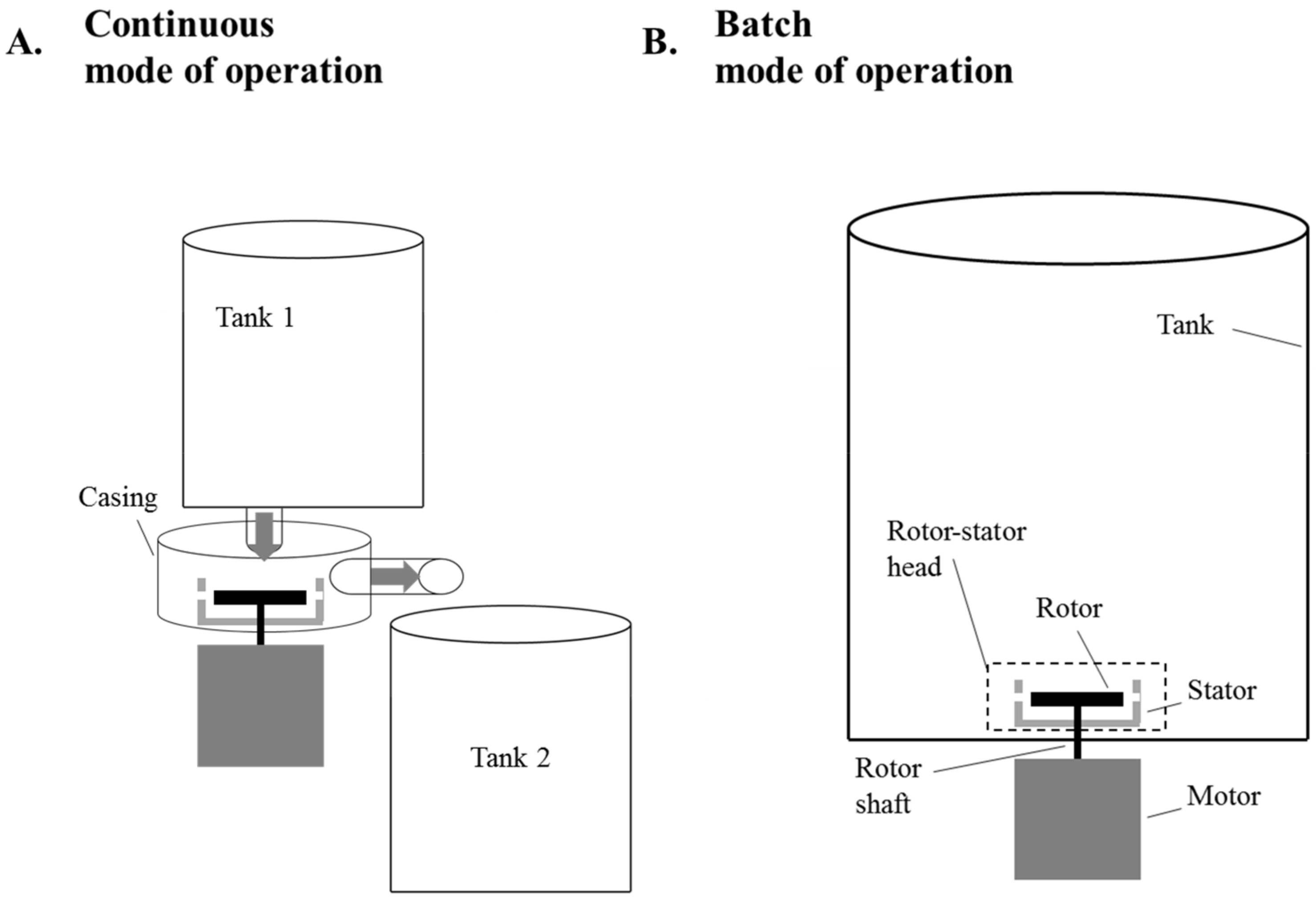
Figure 2.
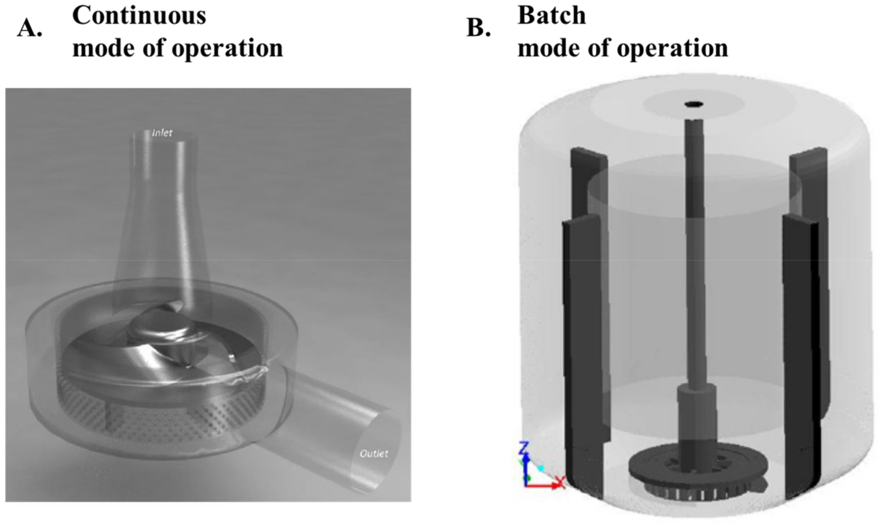
Schematics of RSMs for use in continuous (A) and batch (B) mode of operation.

Figure 3.
Schematic representation of a rotor-stator head with blade-design (A) and teeth-design (B). D denotes the rotor diameter, and δ denotes the rotor-stator clearance.
Figure 3.
Schematic representation of a rotor-stator head with blade-design (A) and teeth-design (B). D denotes the rotor diameter, and δ denotes the rotor-stator clearance.
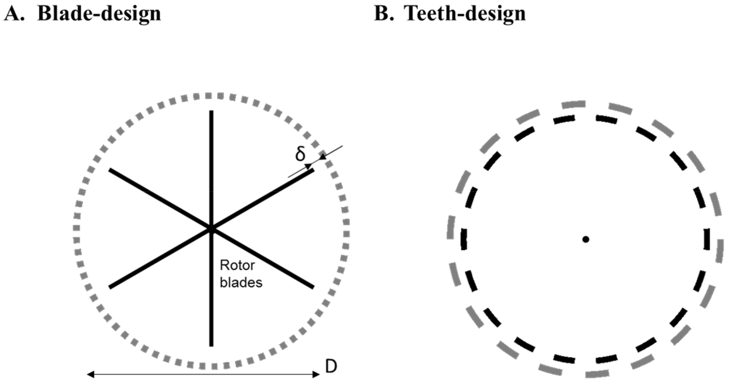
Figure 4.
Velocity fields calculated using computational fluid dynamics (CFD) for two rotor-stator heads. (A) The flow field in a blade-design (Silverson RSM), reproduced with permission from [16], published by Elsevier, 2015; (B) The flow field in a teeth-design (Fluko RSM) from Xu et al. [11], reproduced with permission from [11]; published by Willey Online Library, 2013. Both show systems with two rows of rotor-stators.
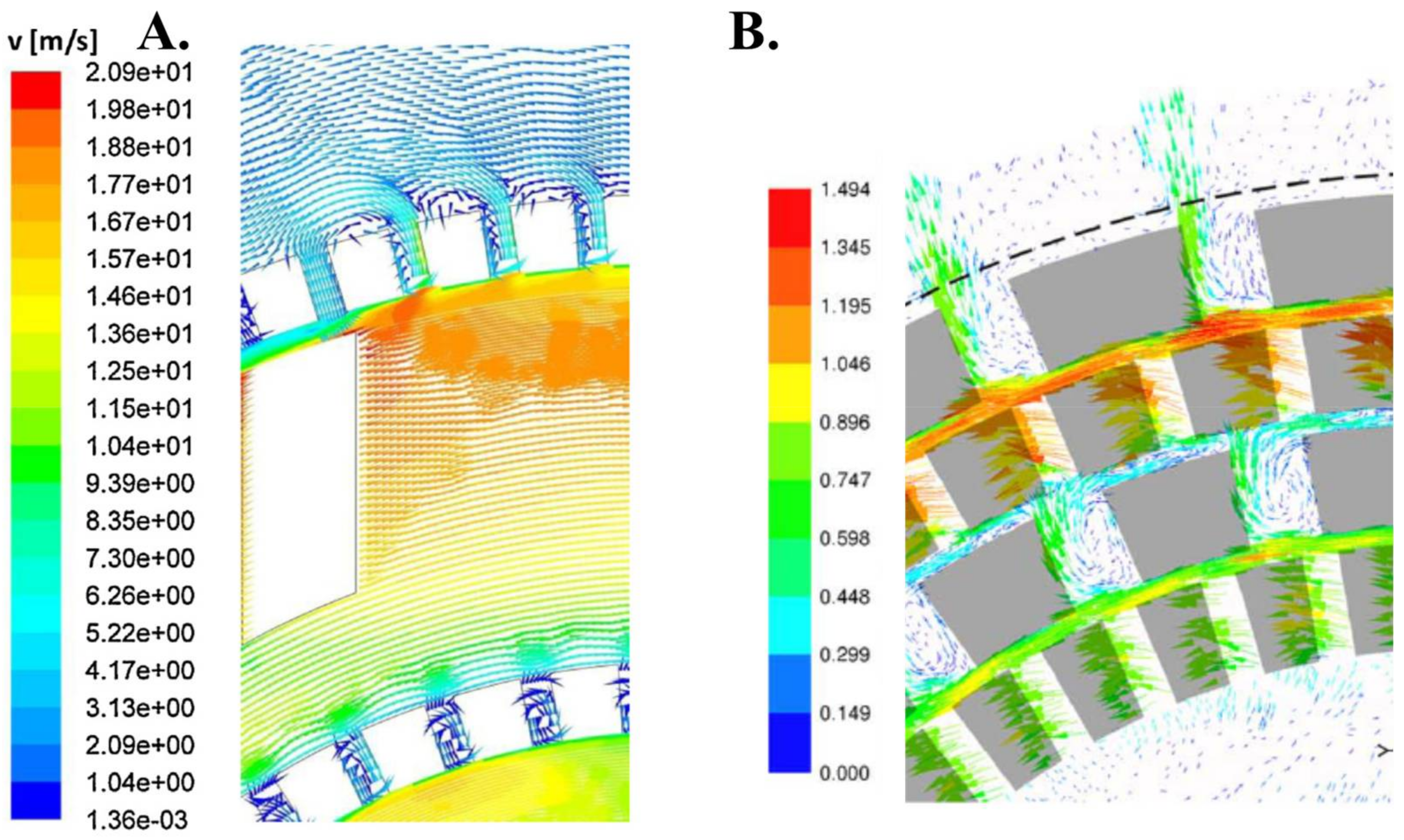
Figure 5.
(A) Plot of Equation (11) to determine the pump constants c1 and c2 for the five mixers in Table 1. (Ppump denotes the pumping power of the mixer and Πflow denotes the flow-term in the power-draw correlation, see Section 5.2.) (B) Pumping efficiency (ηpump) as a function of the flow number (NQ) for the five mixers, compared to data for a typical centrifugal pump. Data from [27,34,36]. See Reference [35] for the methodology.

Figure 6.
CFD-estimated dissipation rates of turbulent kinetic energy TKE in the stator slot region for the same rotor-stator head run at a flow number corresponding to an RSM run under continuous mode of operation (A) and run under batch mode of operation (B). Adapted from data obtained in Reference [54].


Table 1.
A comparison of power and pumping characteristics of some continuous mode rotor-stator mixers (RSMs).
Table 1.
A comparison of power and pumping characteristics of some continuous mode rotor-stator mixers (RSMs).
| RSM | Power Characteristics | Pumping Characteristics * | Ref. | Figure 5 ** | |||||
|---|---|---|---|---|---|---|---|---|---|
| Rotor | Stator | Manufacturer | D (m) | NP0 | NP1 | c1 | c2 | ||
| Blade | Circular holes | Tetra Pak | 0.20 | 0.11 | 9.2 | 0.46 | −3.8 | [36] | I |
| Blade | Square holes | Fluko | 0.060 | 0.24 | 8.4 | 0.24 | −1.1 | [27] | II |
| Blade | Circular holes | Silverson | 0.12 | 0.10 | 6.4 | 0.44 | −3.2 | [34] | III |
| Teeth (1 row) | Teeth | Ystral | 0.12 | 0.13 | 9.7 | 0.23 | −2.4 | [34] | IV |
| Teeth (2 rows) | Teeth | Fluko | 0.060 | 0.15 | 14.5 | 0.13 | −4.5 | [27] | V |
* See Section 5.2 for definitions and a discussion on pumping characteristics. ** Relates the five mixers to the graphs in Figure 5.
Table 2.
Flow numbers (NQ) for a number of batch and continuous mode RSMs.
| RSM | Rotor Speed, U (m/s) | NQ (-) | Method * | Ref. | |||
|---|---|---|---|---|---|---|---|
| Rotor | Stator | Manufacturer | D (m) | ||||
| Batch Mode of Operation | |||||||
| Blade | Rectangular slots | Tetra Pak | 0.20 | 3–14 | 0.11 | PIV | [8] |
| Blade | Rectangular slots | Tetra Pak | 0.20 | 3–14 | 0.11–0.15 | PIV | [9] |
| Blade | Circular holes | Silverson | 0.0028 | 3–5 | 0.22 | LDA | [12,38] |
| Blade | Rectangular slots | Silverson | 0.0028 | 6 | 0.18 | CFD | [17] |
| Blade | Square holes | Silverson | 0.0028 | 6 | 0.26 | CFD | [17] |
| Inline Mode of Operation | |||||||
| Blade | Circular holes | Tetra Pak | 0.20 | 20 | 0.02–0.06 | - | [3] |
| Blade | Circular holes | Silverson | 0.040 | 6–22 | 0.0003–0.037 | - | [39] |
| Blade | Circular holes | Silverson | 0.022 | 5–12 | 0.0003–0.0095 | - | [39] |
| Blade | Circular holes | Silverson | 0.0038 | 6–10 | 0.002–0.04 | - | [16] |
| Blade | Circular holes | Silverson | 0.12 | 13–19 | 0.0005–0.08 | - | [34] |
| Teeth | Teeth | Ystral | 0.12 | 13–19 | 0.0005–0.08 | - | [34] |
| Teeth | Teeth | Fluko | 0.060 | 5–10 | <0.05 | - | [27] |
| Blade | Circular holes | Fluko | 0.060 | 5–10 | <0.05 | - | [27] |
* Method used for obtaining the flowrate through the stator slots in batch mode of operation: PIV (particle image velocimetry), LDA (laser Doppler anemometry) and CFD (computational fluid dynamics). (For continuous mode of operation, the flowrate is an externally measureable parameter).
© 2018 by the author. Licensee MDPI, Basel, Switzerland. This article is an open access article distributed under the terms and conditions of the Creative Commons Attribution (CC BY) license (http://creativecommons.org/licenses/by/4.0/).
Share and Cite
MDPI and ACS Style
Håkansson, A. Rotor-Stator Mixers: From Batch to Continuous Mode of Operation—A Review. Processes 2018, 6, 32. https://doi.org/10.3390/pr6040032
AMA Style
Håkansson A. Rotor-Stator Mixers: From Batch to Continuous Mode of Operation—A Review. Processes. 2018; 6(4):32. https://doi.org/10.3390/pr6040032
Chicago/Turabian StyleHåkansson, Andreas. 2018. "Rotor-Stator Mixers: From Batch to Continuous Mode of Operation—A Review" Processes 6, no. 4: 32. https://doi.org/10.3390/pr6040032
Note that from the first issue of 2016, this journal uses article numbers instead of page numbers. See further details here.